Article

Evolution of Plume Core Structures and Turbulence during a Wildland Fire Experiment

by
Maritza Arreola Amaya
and
Craig B. Clements
*
Fire Weather Research Laboratory, Department of Meteorology and Climate Science, San José State University, San José, CA, 95112, USA
*
Author to whom correspondence should be addressed.
Atmosphere 2020, 11(8), 842; https://doi.org/10.3390/atmos11080842
Submission received: 25 June 2020 / Revised: 5 August 2020 / Accepted: 6 August 2020 / Published: 9 August 2020
(This article belongs to the Special Issue Atmospheric Turbulence Processes and Wildland Fires)

Abstract

:
Micrometeorological observations were made during a prescribed fire experiment conducted in a region of complex terrain with grass fuels and weak ambient winds of 3 m s−1. The experiment allowed for the analysis of plume and turbulence structures including individual plume core evolution during fire front passage. Observations were made using a suite of in situ and remote sensing instruments strategically placed at the base of a gully with a 24° slope angle. The fire did not spread upwards along the gully because the ambient wind was not in alignment with the slope, demonstrating that unexpected fire spread can occur under weak wind conditions. Our observational results show that plume overturning caused downward heat transport of −64 kW m−2 to occur and that this mixing of warmer plume air downward to the surface may result in increased preheating of fine fuels. Plume evolution was associated with the formation of two plume cores, caused by vigorous entrainment and mixing into the plume. Furthermore, the turbulence kinetic energy observed within the plume was dominated by horizontal velocity variances, likely caused by increased fire-induced circulations into the plume core. These observations highlight the nature of plume core separation and evolution and provide context for understanding the plume dynamics of larger and more intense wildfires.

1. Introduction

Wildland fires can modify the atmospheric environment in the near vicinity of the fire front by the formation of fire-induced winds and indrafts [1]. These winds have been linked to modifying fire behavior and cause high rates of fire spread in extreme cases [2]. While there has been an increase in understanding of the role fire–atmosphere interactions have on fire spread using coupled fire–atmosphere models [3,4], there is a continuing need for high spatial and temporal resolution observations of both plume structure and micrometeorology of the fire environment to better understand the physics of both fire spread and plume dynamics [5,6]. To date, a number of field experiments have been conducted to address this need; however, few observations have been able to measure the structures within the plume core, which are required in order to account for changes in fire behavior associated with more complex environments [2].
Small-scale field experiments, defined generically as a burn unit with a horizontal scale of ~1 km2 or less, have been critical in observing key turbulent structures associated with the fire front and fire spread. This is because a large array of instrumentation can be deployed strategically within the fuels to allow the fire front to pass through the instrumentation. A varying level of complexity can be achieved by using sites with various fuel types [7,8,9,10], more complex terrain [11], and high wind conditions [5]. These experiments have led to improved understanding of fire–atmosphere interactions associated with fire spread. For example, in a small burn on a slope with a cross-wind, cross-slope momentum transport that reached the surface layer was caused by along-wind vorticity within the plume [11]. However, there still remain poorly observed and understood plume processes including the accelerating updraft and its dynamics, the surface inflow winds including the rear inflow into the fire front, and turbulence generated at the head of the fire [1,12].
Plume structures have been observed in greater detail using Doppler lidar during both prescribed, experimental fires [5,13,14] and wildfires [15,16,17,18]. It was found that, during a low-intensity, prescribed fire, Doppler-measured radial wind velocities accelerated into the upwind side of the plume column and then decreased downwind of the plume, indicating that a convergence region formed at the base of the plume with a maximum convergence of −0.14 s−1 adjacent to the fire front [13]. In another study using a scanning Doppler lidar [16], it was found that the mean plume structure fit the expected form of a bent-over plume in a crosswind. The data from the lidar were used to estimate the heat flux that must have been responsible for the observed plume behavior by fitting the Briggs plume-rise equation.
The thermodynamic structures within plumes have also been measured during grass fires [19] and low-intensity subcanopy fires [10]. During the subcanopy fires the observed updraft velocities within the canopy were in the range of 2 to 4 m s−1, with fireline intensities ranging from 1200 to 2500 kW m−1. Downdrafts of colder air into the canopy were observed to occur where larger fireline intensities were associated with increased downward momentum transfer. With this increased downward motion, horizontal surface winds also increased. These observations suggest a link between the plume core and the near-surface environment which likely influences fire spread. While this has been suspected to occur in larger wildfires, small-scale field experiments allow for highly resolved observations to be made using a range of instrumentation optimally arranged to sample plume structures and fire behavior.
In this paper, we present experimental field observations of the micrometeorology of a fire plume obtained during a small experimental grass fire that was intended to spread up and through a narrow gully on a slope. The following sections of the paper discuss the experimental design and instrumentation, the results of the observations including turbulence statistics and the plume two-core structure observed by Doppler lidar, followed by the conclusions.

2. Methods and Experimental Design

A field experiment campaign was designed to measure the micrometeorology associated with fire spread on a simple slope. Two field experiments took place at the U.S. Army Garrison Fort Hunter Liggett in Central California (Figure 1) on 20 and 22 June 2012. The experiment on 22 June is described in this paper and was one of the two burns conducted at different sites. The goal of the experiments was to study the micrometeorology of fire spread on slopes. In this experiment, basic fire characteristics and associated micrometeorology were measured as the fire front spread through an instrumentation array. While the overall goal was to collect measurements of the fire spread on the slope, the data presented here represent only those data measured as the fire spread on a low-angle area at the base of steep hill. The experimental layout is shown in Figure 1 and Figure 2.

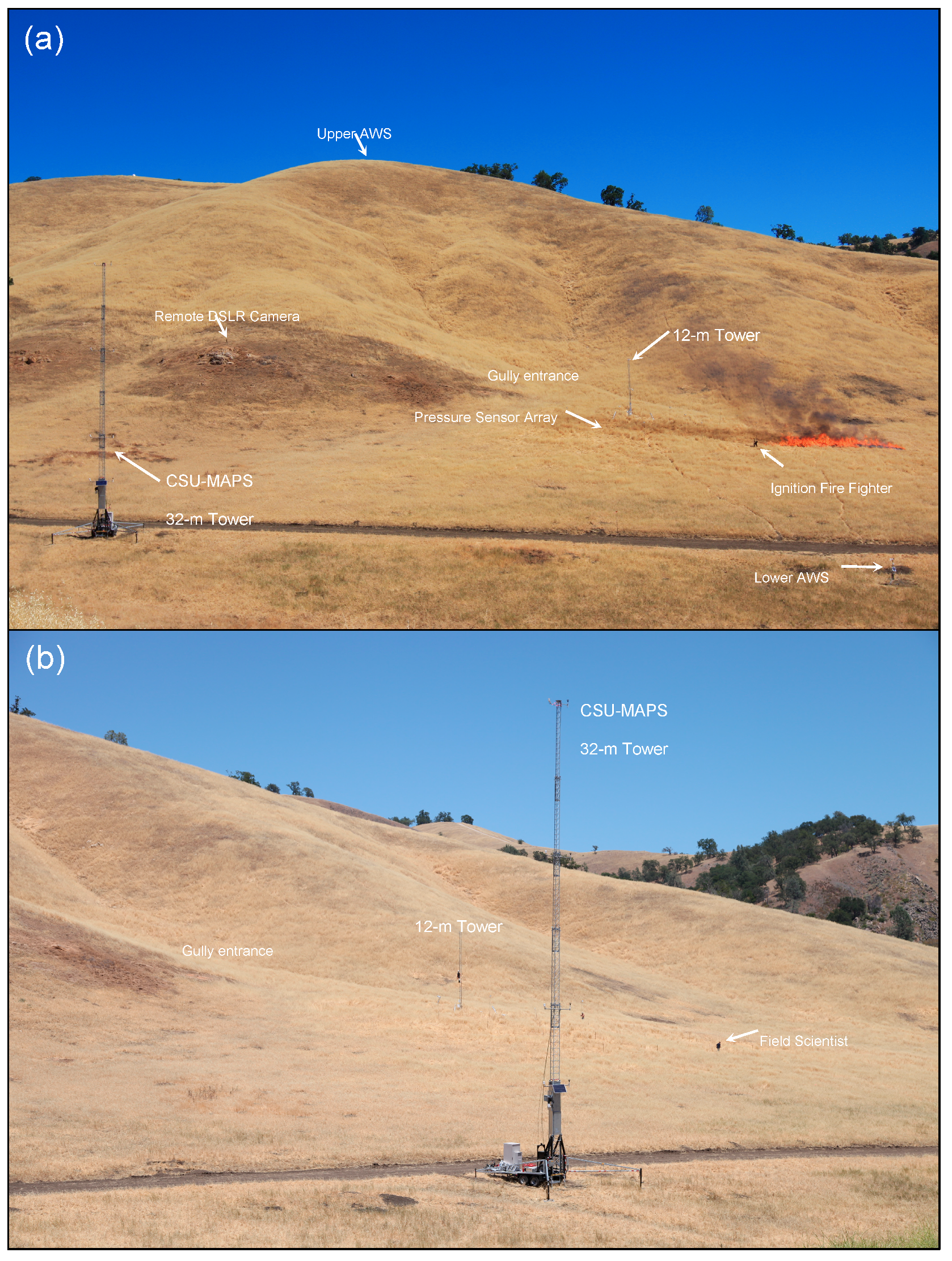
2.1. Site Characterization

The experimental site was characterized as an oak savanna woodland dominated by tall grass with sparse oak trees. The experimental plot was located at the base of a steep hill on a flat area with a slope of ~8° (Figure 2a,b). The hill was incised by a shallow ravine or gully where the lower and upper sections of the gully had slope angles of 22° and 24°, respectively. The anticipated fire spread direction was up the gully, but the ambient wind direction (cross-slope) prevented the fire front from spreading up the slope until extra ignition flares were used in the gully.

2.2. Fuels

Fuels consisted of fully cured California oatgrass (Danthonia californica) that was fairly uniform across the plot, except for some patchy areas on the western shoulder of the gully. Fuel loading was measured using 20 sample plots of 0.25 m2. The sample plots were arranged with half of the sample plots located on the flat area and the other half on the slope. The mean fuel loading was 1.9 tons acre−1 (0.11 kg m−2), with a minimum and maximum of 0.80 and 3.82 tons acre−1, respectively. The fuel coverage averaged 82%, with maximum coverage of 100% and a minimum of 40% of that of bare soil. The average height of the grass was 60.8 cm, with maximum and minimum heights of 94 and 31 cm, respectively.

2.3. Instrumentation

A suite of instruments was used to measure the micrometeorology and structure of the plume, including both in situ and remote sensing sensors. To characterize the ambient meteorology of the site, two automatic weather stations (AWS) were placed near the burn unit, one located near the ignition line and approximately 100 m from the bottom of the slope and the other at the top of the slope (Figure 1 and Figure 2). These two stations were equipped with a data logger (Campbell Scientific, Inc. (CSI), CR1000, Logan, UT, USA), a temperature and relative humidity sensor (CSI, CS215), and an anemometer (R.M. Young 5103). The anemometer was mounted on an aluminum tripod at 3 m above ground level (AGL) and the temperature and relative humidity sensor was mounted at 2 m AGL. The sensors were sampled at 1 Hz, and 5-min averages were recorded and stored. Additionally, profiles of wind speed and direction, temperature, and relative humidity (RH) were measured using the California State University Mobile Atmospheric Profiling System (CSU-MAPS, [20]) 32 m meteorological tower that was positioned outside the burn unit (Figure 2a). This tower was equipped with 2-D sonic anemometers (Gill Instruments, WindSonic, model 1405-PK-021) and Vaisala, Inc., HMP45C temperature and humidity probes. The sensors were mounted on cross-arms at heights of 7, 12, 22, and 32 m AGL. These sensors were sampled at 1 Hz using a CSI CR1000 data logger and data were stored at 1 Hz. Finally, wind profiles were measured using an acoustic Doppler sodar (Atmospheric Systems Corp., model 4000) which provides 10-min averaged vertical wind profiles of the three-dimensional winds from 15 to 200 m AGL. Upper-air measurements were also made using a Vaisala, Inc, RS92G radiosonde that was launched at 0900 PST near the burn unit (Figure 1, lidar location) and a Radiometrics, Inc, MP3000A microwave temperature and humidity profiler was operating continuously throughout the experimental period. Sensor and instrument specifications are listed in Table 1.
Inside the burn unit, a 12-m tower was installed to measure the micrometeorology of the fire front and the turbulence within the plume. In addition to the tower, an array of temperature-pressure sensors was installed in a grid to measure the pressure perturbations associated with the fire front. These sensors were custom-built and are described in [5]. To measure the three-dimensional winds, turbulence, and heat flux within the plume, a 3-D sonic anemometer (Applied Technologies, Inc., model SATI-Sx, Cleveland, OH, USA) was installed at 12 m AGL. In addition, plume temperatures were measured using fine-wire thermocouples (Omega, Inc., 5SC-TT-E-40, Norwalk, CT, USA) mounted ~ every meter along the tower length from 1–10 m AGL. Heat flux radiometers (Hukseflux Thermal Sensors, SBG01; Medtherm, model 64, Delft, Netherlands) were mounted on the tower at 3 m AGL using a cross arm that allowed the sensors to measure the fire from above, with the sensors pointed nadir towards the surface. All sensors were sampled at 10 Hz using a CSI CR3000 data logger, with the exception of the fine-wire thermocouples, which were sampled at 5 Hz. These high-frequency samples were stored on a data card in the data logger for later download.
Plume structure was also sampled using a scanning Doppler lidar (Halo Photonics, Ltd., Streamline 75) which was located on a hill approximately 200 m south of the burn unit (Figure 1). The lidar was configured to scan vertically through the plume using range height indicator (RHI) scans (dashed line indicated in Figure 1). More information regarding the lidar system and its application for plume monitoring can be found in [13,16].

2.4. Data Processing

The high-frequency data were processed following [11,21]. The raw time series data of u, v, w, Ts (sonic temperature) were processed to eliminate spikes, using 4σ of the value. If a value was outside this limit, it was considered a spike and this data point was replaced with the average of the five values preceding and succeeding this data point. After despiking, the data were then rotated into stream-wise coordinates and tilt corrected following [22], where u is the streamwise component and v is the cross-wise component. These processed data were subsequently used for the turbulence statistics to analyze the plume and micrometeorological aspects of the fire front passage (FFP). Turbulence statistics including the velocity variances u 2 ¯ ,   v 2 ¯   ,   w 2 ¯   and turbulence kinetic energy,   e = 0.5 ( u 2 ¯ + v 2 ¯ + w 2 ¯ ) , were calculated from the processed 10 Hz time series data of u, v, w, and Ts. In order to isolate the turbulence associated with the FFP, a short Reynold’s average period of 10 s was used, which is indicated by the overbar, and the prime indicates the perturbation of each variable. Additionally, the turbulent sensible heat flux, H s = ρ c p w T s ¯ , was calculated using a 10-s running average and defined as the covariance of the perturbation temperature and vertical velocity multiplied by the density of air, ρ, and the specific heat capacity of dry air at constant pressure, cp, 1004 J kg−1 K−1.

2.5. Ignition Procedure

The ignition was conducted with a single fire fighter using a drip torch and a flare gun. The initial ignition line was aligned perpendicular to the slope and the fire was allowed to spread towards the 12-m tower. Since the fire front did not continue to spread towards the slope initially, the firing pattern and ignition had to be modified so that the ignition line was then wrapped around to the southeast of the tower. The ignition was later enhanced by the use of ignition flares that were fired in order to land within the gully, and this occurred after the main fire front had moved through the 12-m tower and instrumentation array. Multiple flares were used to ignite the slope above the tower to simulate spotting ignition. The fire eventually spread up the slope and two separate head fires merged into one near the top of the slope.

3. Observations and Results

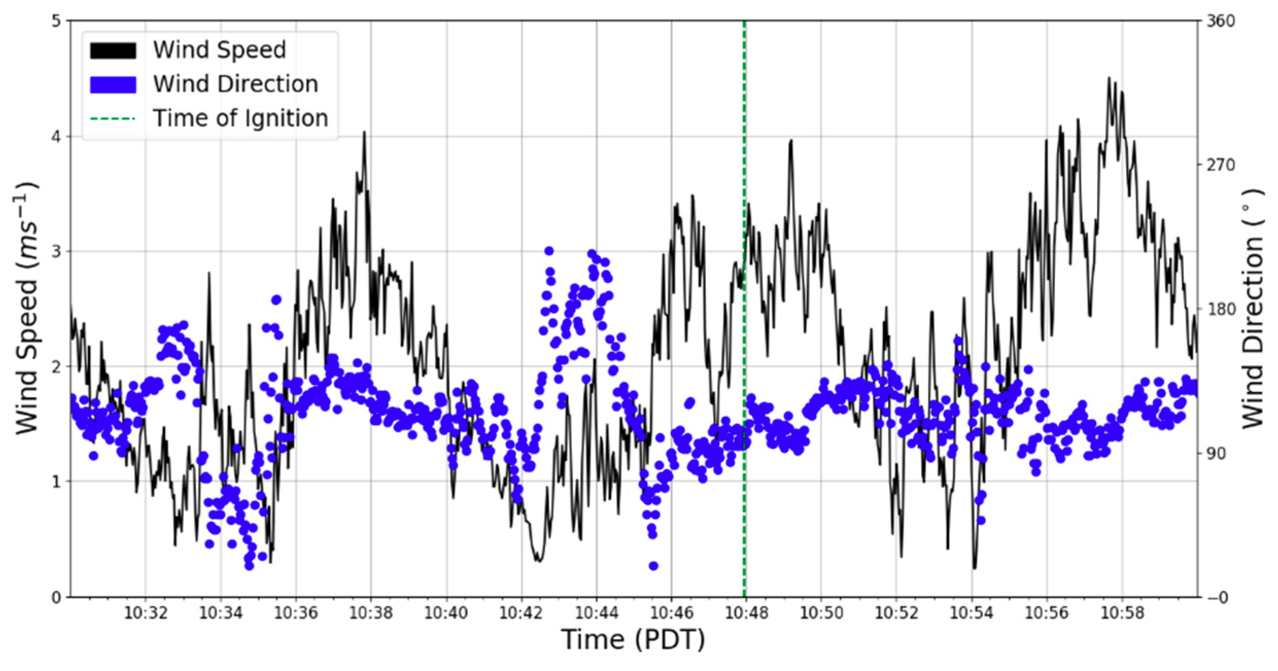
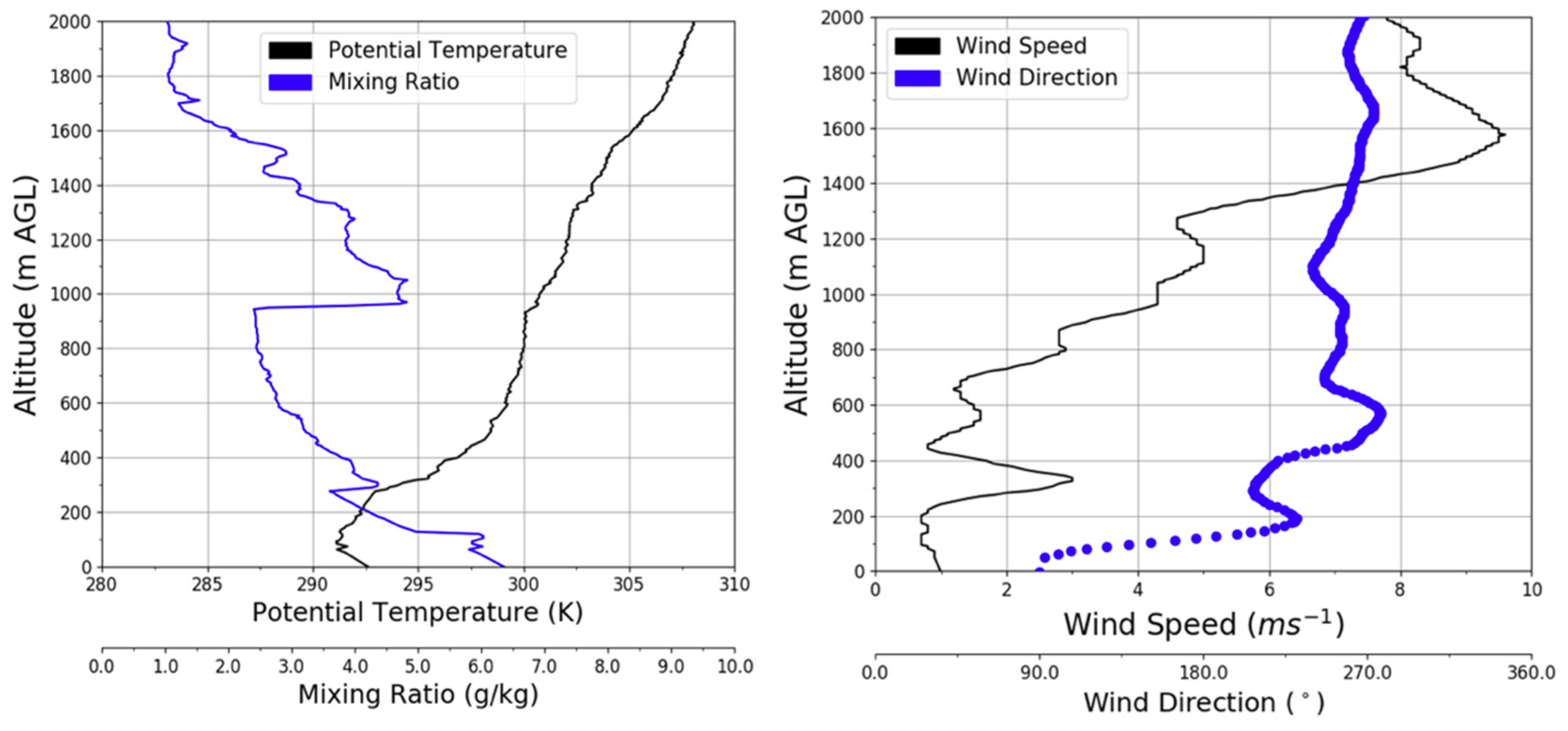
3.1. Background Meteorological Conditions
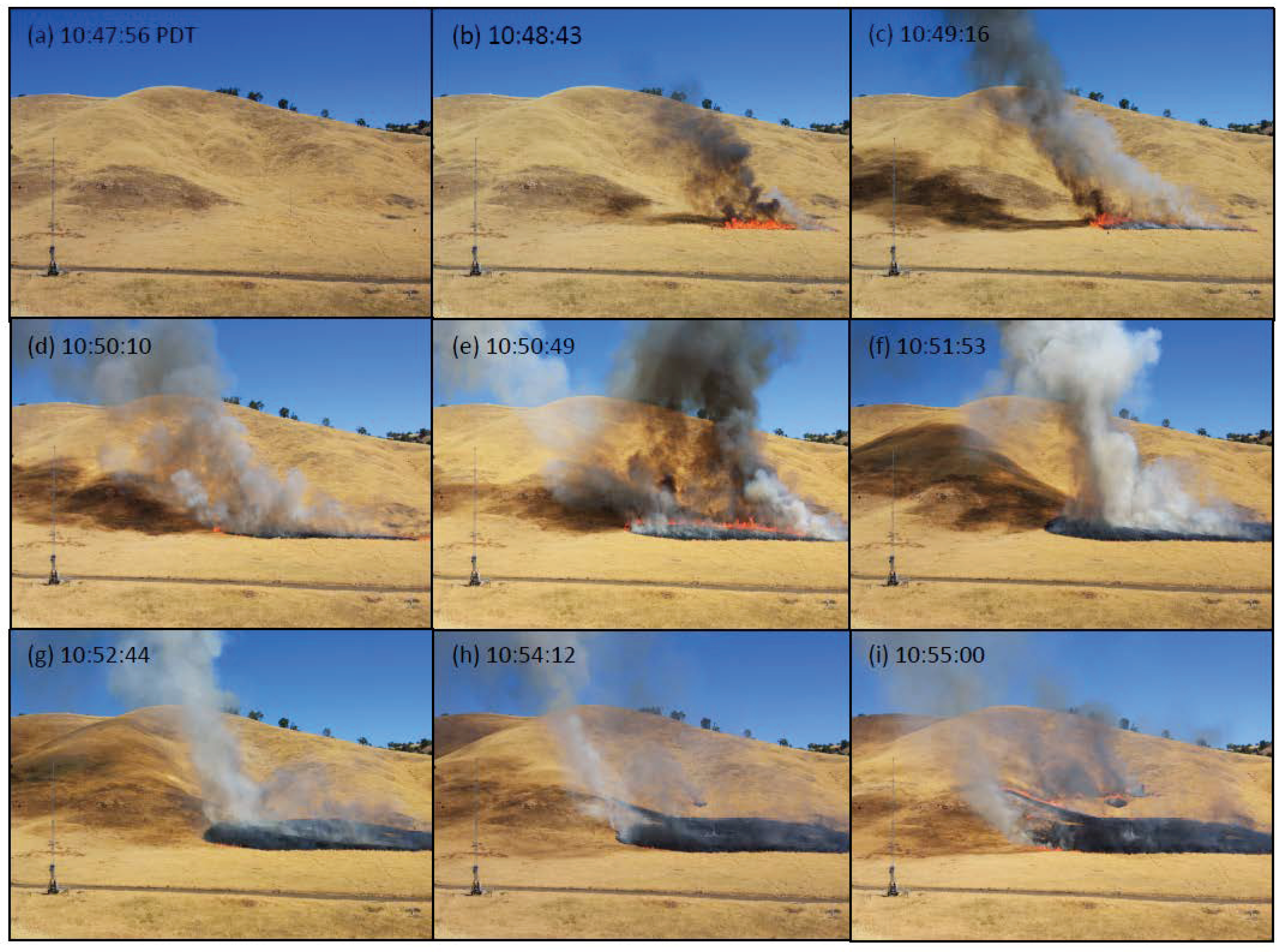
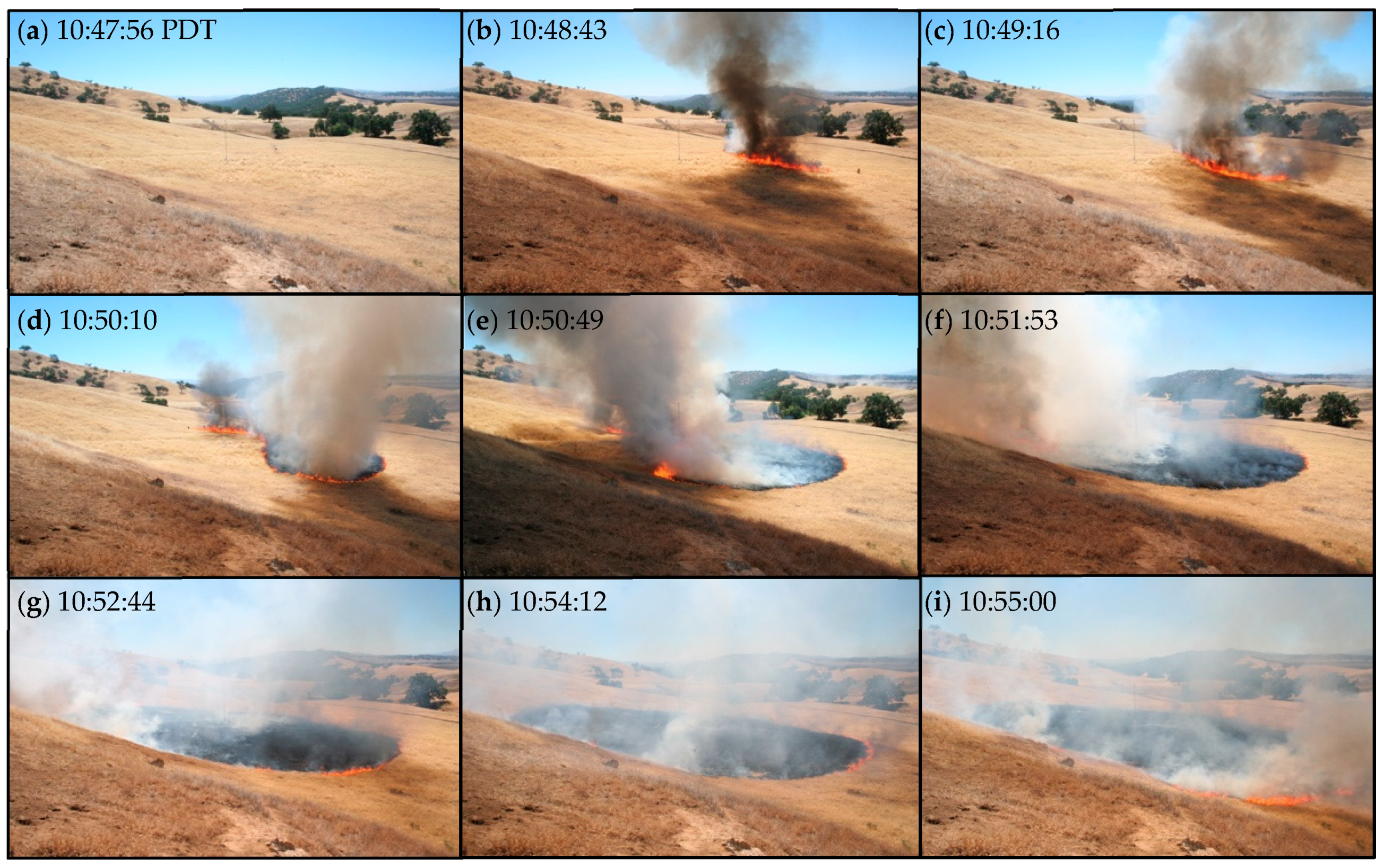
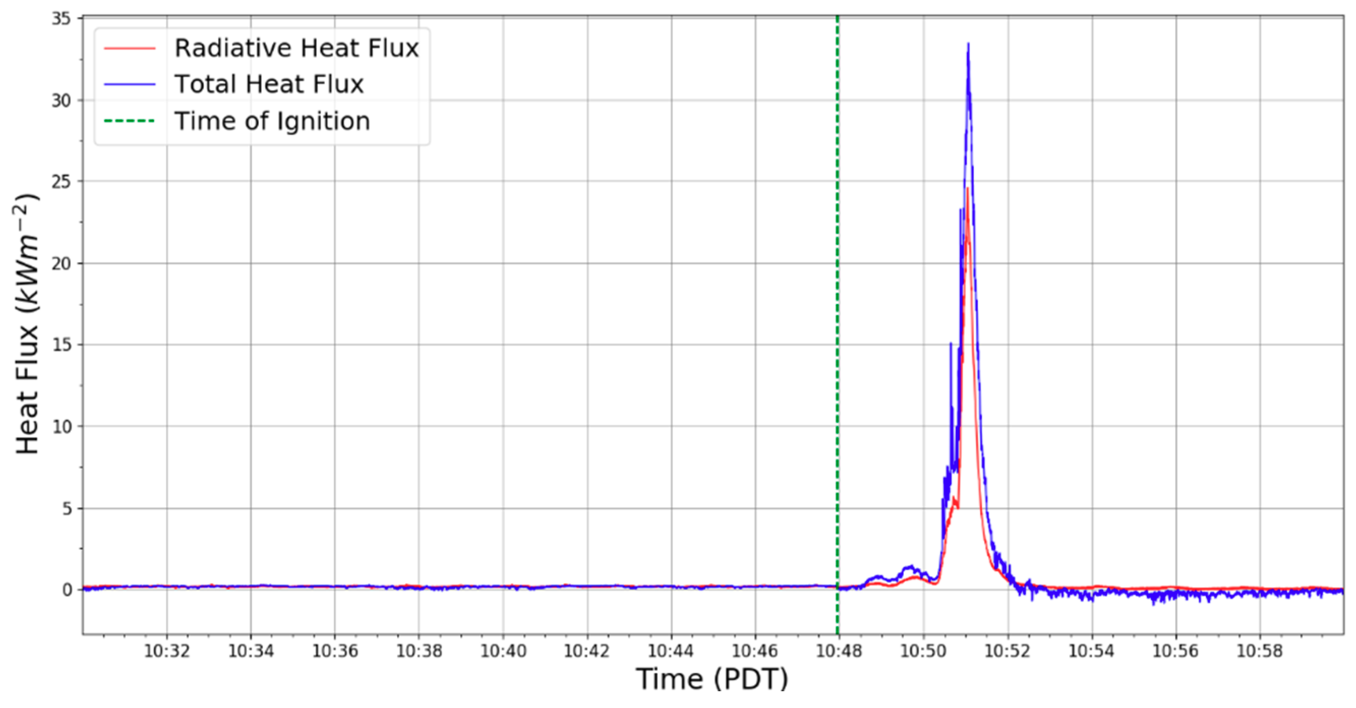
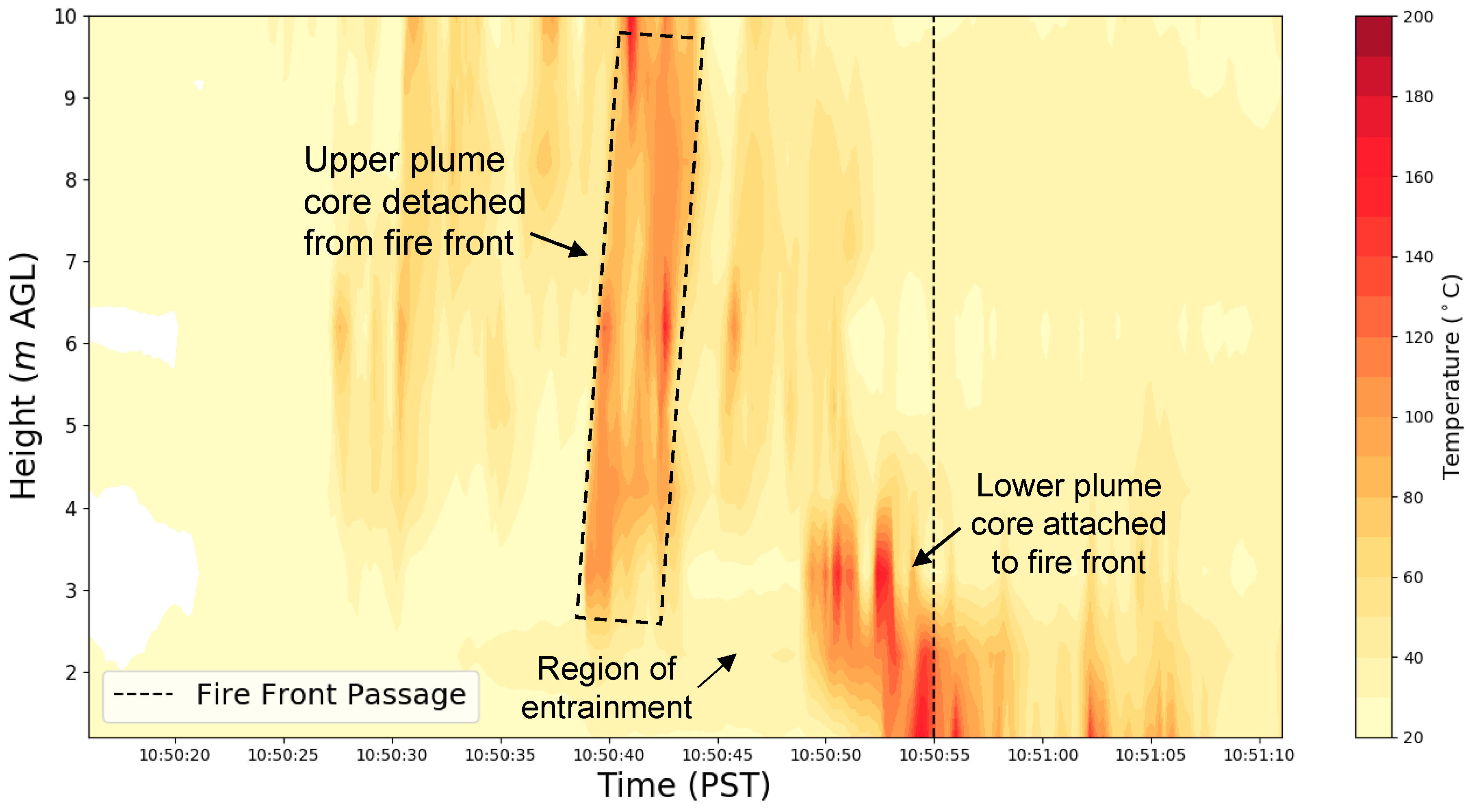
The synoptic environment during the experiment was associated with an upper-level, 500 hPa trough (Figure 3a) located off the California coast, with weak northwest winds at 925 hPa and relative humidity around 20% (Figure 3b). Surface Fosberg Fire Weather Index [23] (Figure 3d) values were low, at approximately 10 for the experimental period.
Ambient surface conditions were measured with the two AWS, a Doppler sodar, an upper-air sounding system, and the CSU-MAPS 32-m tower. Figure 4 shows that the surface winds during the experimental period were light and variable, with wind speeds ranging from 1 to 4 m s−1 and southeasterly in direction.
In addition to surface weather conditions, an upper-air sounding was made at 0900 PDT. Figure 5 shows vertical profiles of potential temperature, water vapor mixing ratio, wind speed, and wind direction. There was a strong temperature inversion present between 100 and 500 m AGL, with a near-surface superadiabatic layer present from the surface to the base of the inversion at 100 m AGL representing the erosion of the nocturnal stable layer and the development of a convective boundary layer. Within this layer, the water vapor mixing ratio decreased from 6 g kg−1 at the surface to ~3 g kg−1 at 500 m AGL. The wind speed and wind direction from the radiosonde indicate light winds near the surface ~1 m s−1 that increased above 500 m AGL, with an elevated and shallow low-level jet located between 350 and 450 m AGL. This jet was located within the stable layer and likely represents an intermittent and residual local-scale nocturnal drainage flow associated with the complex terrain of the site. Winds at the surface were southeasterly and southwesterly aloft (Figure 5). The temporal evolution of the vertical wind profile was obtained by the Doppler sodar located southeast of the burn unit (Figure 6). The wind profile within the lowest 100 m AGL was mostly southerly and southeasterly, with light wind speeds of less than 3 m s−1, and remained so during the experimental burn period. The wind profile evolved over time, shifting from more southwesterly to southeasterly, while surface winds near the burn unit indicated that the winds were more easterly during the time of ignition (Figure 4). After 1250 PDT, the winds increased significantly in magnitude and became more westerly and southwesterly and remained like this throughout the afternoon.

3.2. Fire Behavior

Fire behavior was monitored with two synchronized time-lapse cameras (Canon DSL), with one located perpendicular to the rate of spread and the other located farther away and pointed parallel to the fire spread (Figure 7). The images were taken at 1-s intervals and the time stamps were synchronized to the data logger GPS clock during analysis. Figure 7 shows a time series of images taken from the camera located west of the tower on the ridge, where the lidar was located (Figure 1). This image sequence shows the fire spread evolution starting from the ignition procedure through the fire progression as it passed through the 12-m tower. The fire was ignited at 10:47:57 PDT with a single drip torch. At approximately 10:48:43 PDT (Figure 7b), the initial ignition line formed a flanking fire that developed into a head fire that spread towards the 12-m tower. The fire front passage occurred at 10:50:55, as shown in Figure 7e, Figure 8e, and Figure 9. Fire front passage (FFP) is defined as the time that the fire front impacted the tower such that the variable time series is associated with a large perturbation from ambient conditions (Figure 9). This is typically determined using the sonic temperature measured on the tower, as described by [24].
The rate and direction of fire spread were estimated from the time series of photographs in Figure 7 and Figure 8. The rate of spread was estimated to be 0.5 m s−1 through the base of the tower. Flame height and length were estimated from photographs to be 4 m and 7 m, respectively. The surface wind speed at 7 m AGL was approximately 3 m s−1 during the ignition process and the wind direction was southeasterly between 100 and 110°. This wind direction was parallel to the fire ignition line (Figure 1). The fire intensity was determined from radiative and total heat flux radiometers measured during the FFP. The measured total heat flux peaked during the FFP at ~33.5 kW m−2 and the radiative heat flux measured was 24.5 kW m−2. These measurements were made using the heat flux radiometers mounted at 3 m AGL described above and represent the vertical radiative heat flux associated with the fire front as it passed under the tower. The photographic time series in Figure 8 shows the evolution of the fire front shape as the fire progressed underneath the 12-m tower. Initially, the fire spread slowly as a flank fire towards the tower, but soon after, the fire began to spread perpendicular to the tower (Figure 8c) as a head fire. In order to counter this, an additional ignition line was started just before 10:50:10 PDT (Figure 8d) near the heel of the fire forming the eastern flank. This caused the fire front to wrap around the tower (Figure 8d–e) and spread past the tower and towards the gully entrance at 10:51:53 PDT (Figure 8f). At this time, the plume was upright and consisted of a single core (Figure 7f and Figure 8e) before dispersing in response to decreased fire intensity (Figure 7h and Figure 8f).
The duration of the head fire and upright plume structure was short lived, only lasting approximately four minutes once the plume developed upright (Figure 7 and Figure 8). The observed fire spread was likely a result of weak ambient winds, while fire-induced wind velocities were observed to be much higher (~7–8 m s−1) during the FFP (Figure 10), causing the fire front to move towards the slope. This was likely caused by the increase in cross-wise velocity, v (Figure 10). Eventually, the plume dispersed quickly due to decrease in fire intensity resulting from a short period of decreased surface wind speed from 1052 to 1054 PDT (Figure 4).

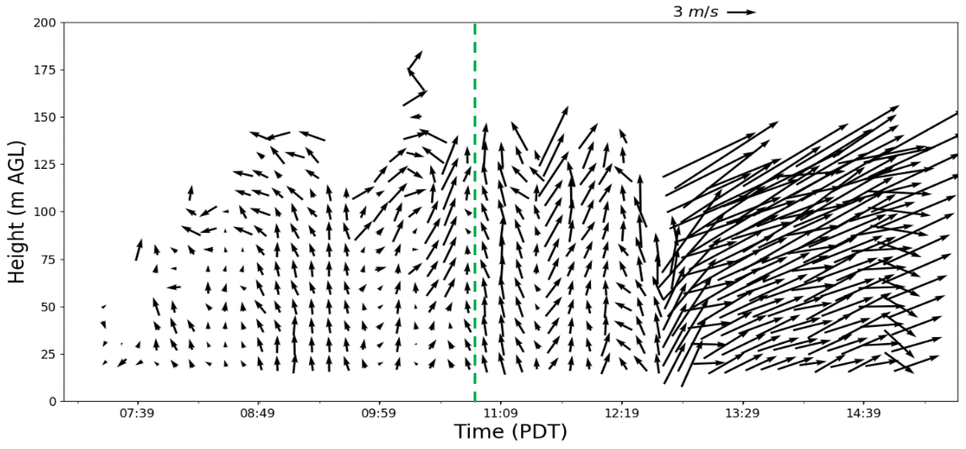
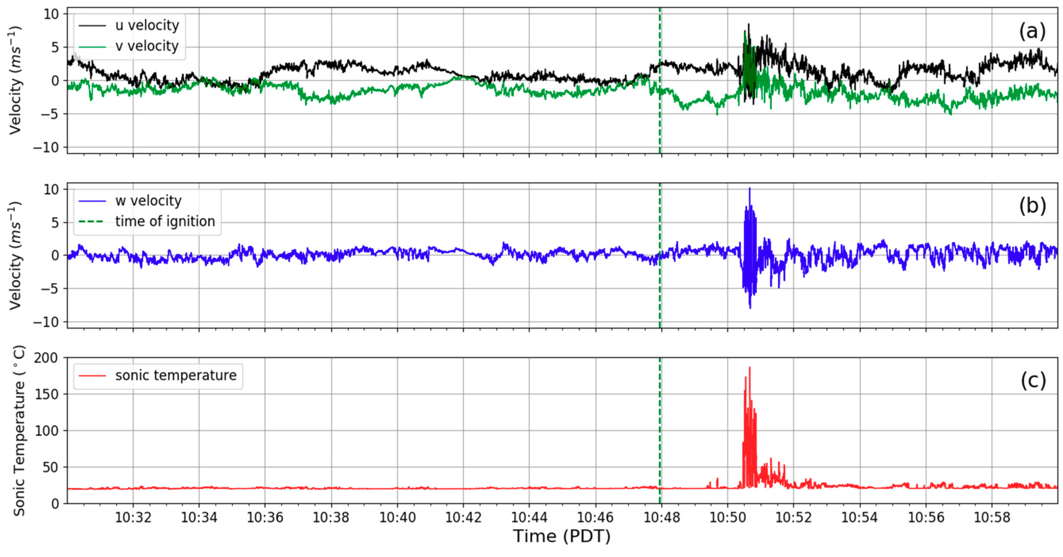
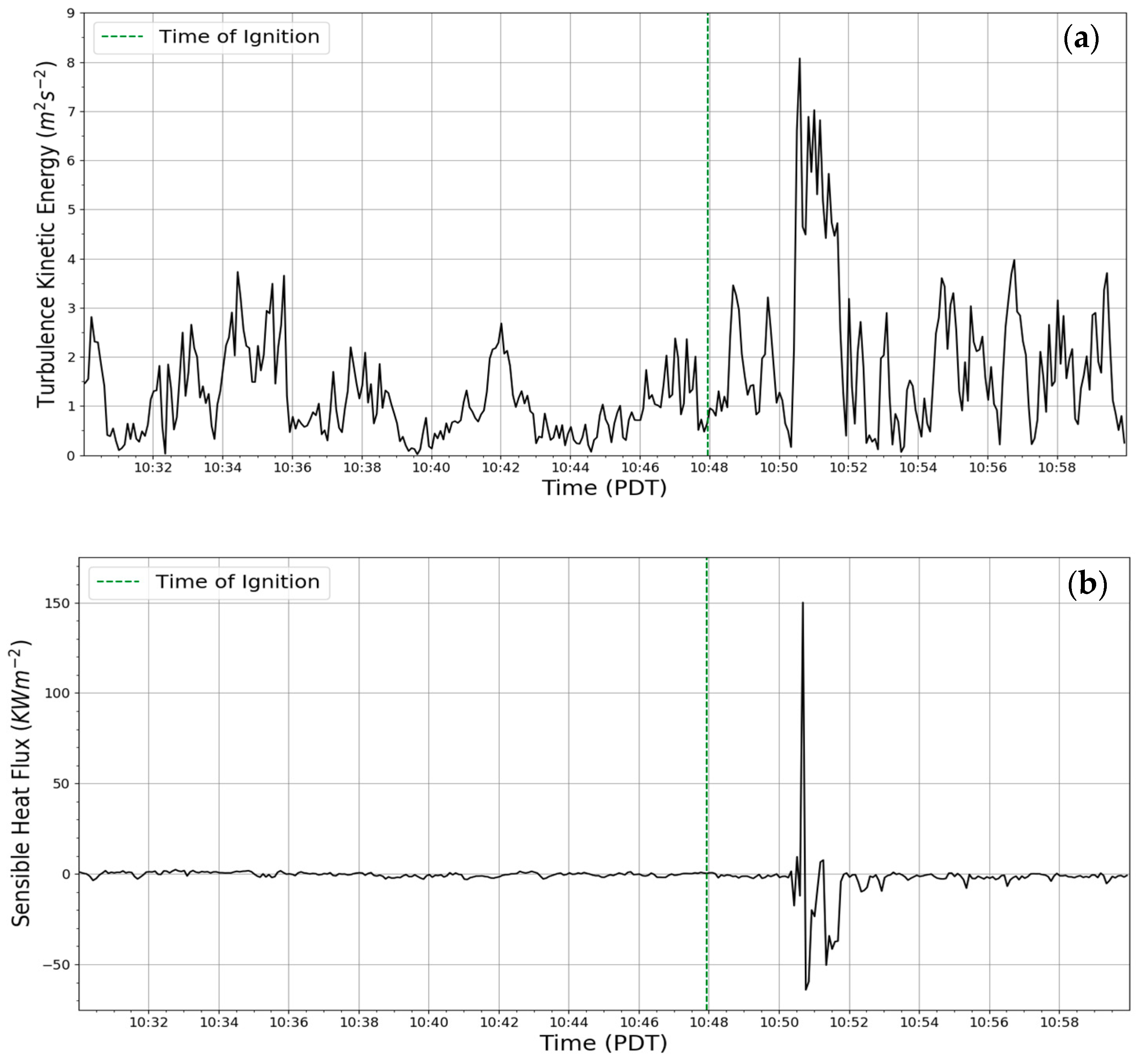
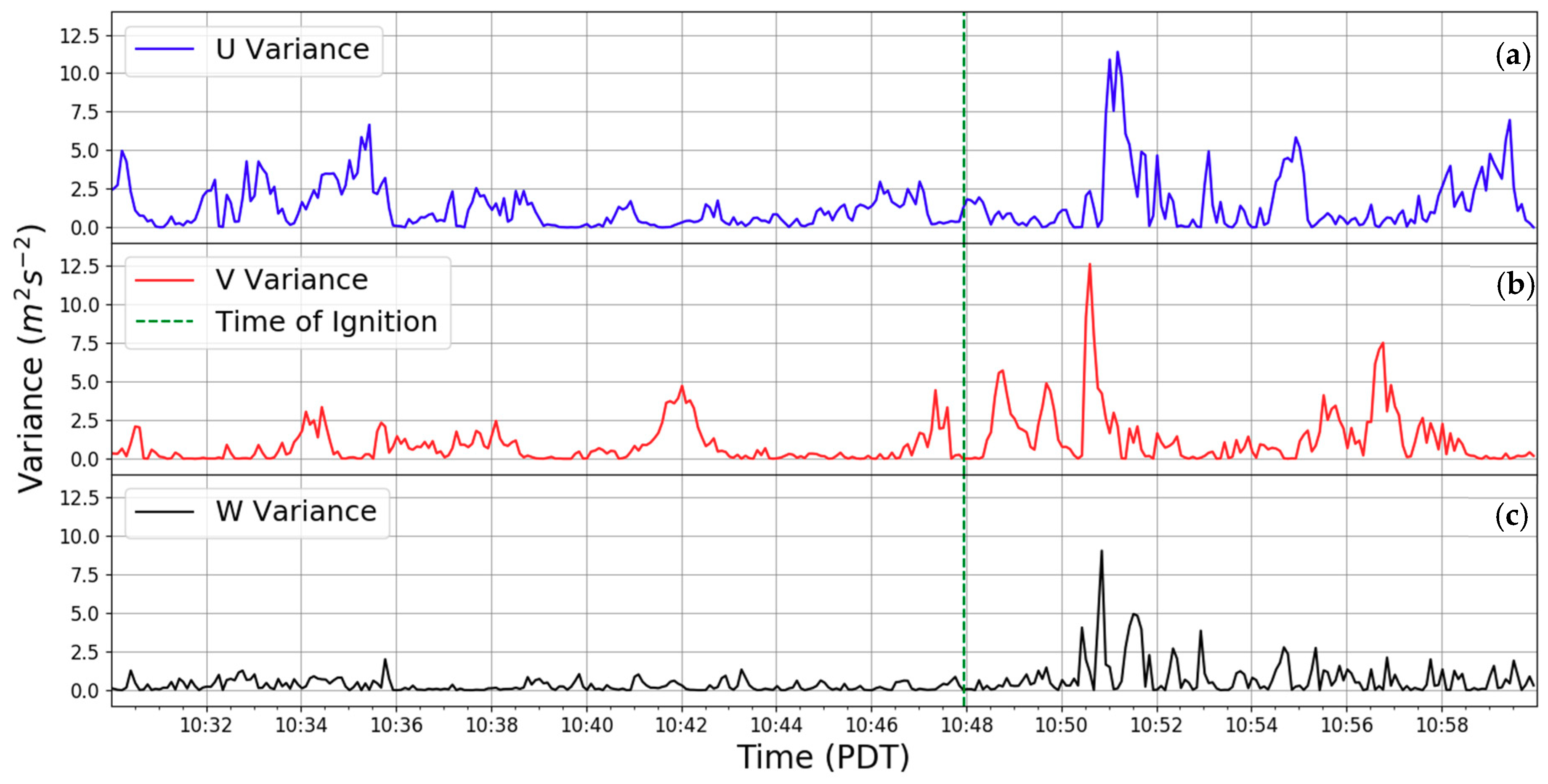
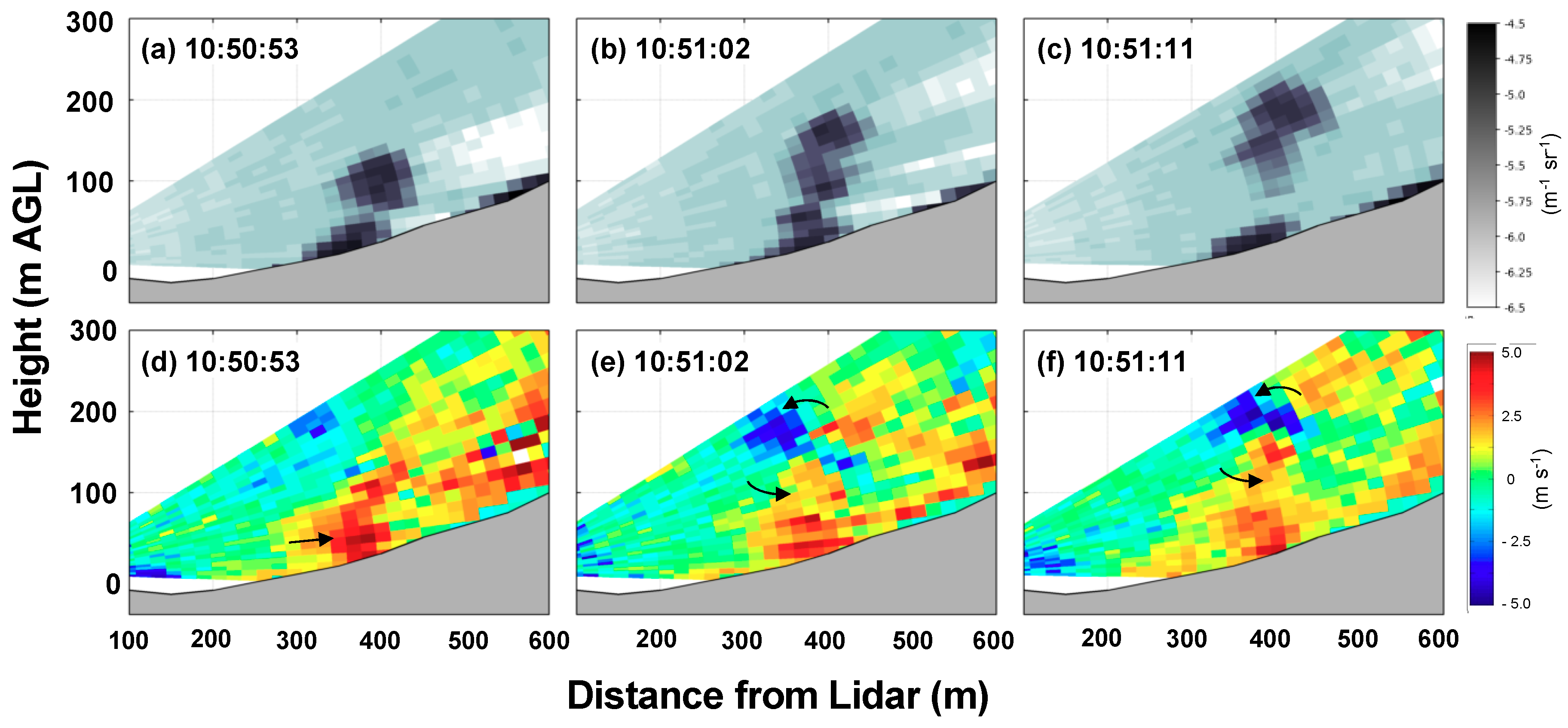
3.3. Plume Micrometeorology

The in situ 12-m tower allows us to describe the turbulence regime of the near-surface plume during the FFP. Since the sonic anemometer was mounted at 12 m, the very near-surface winds were not measured, but the data from the tower (5–12 m AGL) represent the plume base region. Figure 10 shows the period of FFP in the time series of sonic temperature Ts indicated by the sharp increase in temperature. At first, the ambient pre-fire sonic temperature was ~18–20 °C. As the fire spread under the anemometer, the sonic temperature spiked to more than 186 °C and remained above 100 °C for over 15 s, indicating the presence of the plume. After this spike, sonic temperature returned to near ambient as the fire and plume passed. The evolution of the wind field during FFP indicated a strong fire-induced wind within the plume (Figure 10). There is a clear increase in both horizontal (u, v) wind components during the FFP, with the greatest increase from −5.2 to +7.2 m s−1 in the v-component indicating that strong fire-induced indrafts into the plume base from the cross-wise direction occurred. Additionally, the u component velocities increased from −3.6 to +8.5 m s−1 (Figure 10). The vertical velocity during the FFP period was associated with increased updrafts and downdrafts. The updraft magnitude reached a maximum of 10.1 m s−1 and downdrafts reached −8.1 m s−1. These vertical velocities are similar to other observations made during grass fires [5,10,12].
The time series of turbulence kinetic energy (TKE) and sensible heat flux, defined in Section 2.4, are shown in Figure 11. During the pre-fire conditions, the TKE varied between 0.1 and 4 m2 s−2. A peak in TKE is shown during FFP, with the maximum value of 8.1 m2 s−2. After the fire and through midday, there was higher variability of TKE of 0 to 4 m2 s−2 (not shown). Similarly to the TKE results, there was a positive peak in sensible heat flux during FFP that reached 150.1 kW m−2. Seconds later, there was a negative heat flux peak of −64.1 kW m−2, and, a few seconds later, a secondary negative peak of −50 kW m−2 occurred with a longer duration. These negative heat fluxes indicate strong mixing of hot plume air downward towards the surface and may be inferred as entrainment into the plume because it occurred after the initial positive heat flux maximum. The variances of the three wind components are shown in Figure 12. The strongest velocity variance occurred in the v component,   v 2 ¯ , and just before the peak variance in both u 2 ¯   a nd w 2 ¯ occurred. It is interesting to observe that v 2 ¯ increased ahead of u 2 ¯   a nd w 2 ¯ . This is likely due to the fact that fire-induced circulations occurred downwind of the plume as the fire front and plume approached the tower. As soon as the plume impinged on the tower, the u 2 ¯   a nd w 2 ¯ peaked following the initial increase in v 2 ¯ . The dominance of horizontal velocity variance within the plume shows that plume TKE is less isotropic, but this is not due to increased vertical velocity variance.
Plume evolution was observed using the scanning Doppler lidar during the time of the FFP. Figure 13 shows a sequence of RHI scans made during the plume rise, where the plume structure is indicated in the smoke backscatter intensity (Figure 13a–c) and the radial velocities in panels (d–f). From this sequence, the plume rose by approximately 75 m in 9 s from 10:50:53 to 10:51:02 PDT, which equates to a plume rise rate of 8.3 m s−1, which is similar in magnitude to the vertical velocity measured at 12 m AGL on the tower. Additionally, at 10:50:53 PDT, indraft velocities of the near-surface plume increased to ~5 m s−1, as indicated by the arrow in Figure 13d. This period is just after the FFP occurred at the tower and is also corroborated in Figure 8e. At 10:51:02 and 10:51:11 PDT, the radial velocities in the upper region of the plume indicate the presence of horizontal-axis vorticity and overturning of the plume top, as shown by the arrows overlaid on the panels (Figure 13e,f). This overturning suggests strong entrainment and demonstrates the mixing of warm plume air downward that was also observed by the negative sensible fluxes in Figure 11b. Additionally, this is illustrated in Figure 13b, where the smoke backscatter intensity decreased in the middle of the plume. This may be explained by entrainment that caused the plume core to separate from the fire front. This entrainment and plume core separation could have been caused by the increased near-surface indrafts or the plume overturning, or a combination of both. This process may likely help to drive fire spread under weak ambient winds, but this is only speculation.
To better understand the plume core evolution, the thermodynamic structure of the plume was analyzed using the fine-wire thermocouple data obtained from the in situ tower (Figure 14). These data were recorded at 5 Hz and therefore provide a high temporal and spatial (1 m in the vertical) view of the plume temperature evolution. In evaluating Figure 14, it is clear that the highest plume temperatures (~170–200 °C) remain near the surface at around 1–2 m AGL and are associated with the fire front. However, it should be noted that flame contact did not occur directly on the thermocouple array, so these temperatures represent the hot gases likely advected ahead of the flame and represent the time of FFP. This process has been observed in previous field experiments [5,11,19]. One of the most notable features in the observed thermal structure is the sharp discontinuity in the vertical temperature structure identified by the two separate plume cores of higher temperatures. The upper core is the plume that has separated from the fire front, while the lower core is attached to the fire front. This dual-core structure is caused by entrainment and mixing of ambient air into the plume. This thermal structure is also observed in the lidar backscatter (Figure 13a,c), where clearer air, represented by lower backscatter intensity, is observed between two larger plume cores. The two separate plume cores in the lidar backscatter are much larger in spatial scale, both horizontally and vertically. Comparing both the lidar backscatter observations (Figure 13a–c) and the tower thermocouple observations (Figure 14) suggests that the near-surface thermal plume cores grow in size from the surface and fire front to larger plume structures observed aloft by the lidar, a process also observed in much larger plumes associated with wildfires [16]. The plume horizontal spatial structure is not well captured by the tower because it represents a single point in space, while the lidar backscatter shows the scale of the plume boundaries of ~75 × 75 m (Figure 13a–c). In the case of a low intensity fire such as that described in this study, the detached plume is advected away from the fire front as it ascends vertically even under low-wind conditions, whereas under high-wind environments, the plume is also advected near the surface, but the heat transfer remains near the fuel layer, helping to advect ignition temperature gases to unburned fuels ahead of the fire front [5].

4. Conclusions

This study investigated the micrometeorology and evolution of a plume measured during a prescribed experimental grass fire. The experiment was designed to allow for a head fire to move up a narrow gully; however, the prevailing meteorological conditions caused the fire to spread initially as a flank fire which occurred in relatively light winds. While the original goals of the project were not met, the dataset provided a unique analysis of the plume structure as it evolved with time. Our observational results show that, even under light wind conditions, plume mixing caused downward heat transport to occur. Observed negative heat fluxes of −50 and −64.1 kW m−2 represent the mixing of warmer plume air downward to the surface that could increase the preheating of fine fuels. The observed plume evolution was associated with the formation of two coherent plume cores, separated by entrainment and mixing that was caused by plume overturning. The plume overturning was observed by both the Doppler lidar backscatter intensity and radial velocity structures, as well as the temperature time–height evolution. The turbulence kinetic energy within the plume was dominated by the horizontal velocity variances rather than the vertical velocity variance, suggesting that the plume turbulence regime is isotropic, likely caused by plume overturning.
While this field experiment produced an interesting and unique dataset that has allowed a detailed analysis of plume core structure evolution, the intent of the project was to measure the micrometeorology and fire–atmosphere interactions of fire spread in a gully. This failure was caused by changes in the ambient wind but illustrates that fires at the base of a steep canyon or slope do not necessarily spread into the canyon without wind alignment. This finding in itself is not new but further demonstrates the role that complex terrain and its associated wind systems have on fire behavior, including unexpected fire spread even under benign weather conditions. Another unsuccessful aspect of this project that needs to be noted is the fact that fire spread was not adequately sampled to determine the role of fire–atmosphere interactions on fire behavior. For example, airborne imagery of fire front evolution would have provided the necessary data to evaluate fire behavior and fire spread evolution more adequately. Future studies should focus more on observing the fire spread at high temporal and spatial resolution to better understand micrometeorological influences on fire spread.
It should be further noted that the results presented here represent the lower end of the spectrum in terms of fire intensity; however, these observations will likely provide context for other types of fire behavior in complex terrain. For example, the fuels reported here were grass and fairly homogenous, but it could be expected that in different fuel classes such as shrub, the fire intensity would be much higher resulting in larger plume structures and likely more mixing and stronger entrainment. Our results reported here could also be used to constrain future modeling studies which could test the sensitivity of fuel type and fire intensity on plume structure and evolution.

Author Contributions

Conceptualization, C.B.C. and M.A.A.; methodology, M.A.A. and C.B.C.; formal analysis, M.A.A. and C.B.C.; resources, C.B.C.; writing—original draft preparation, M.A.A.; writing—review and editing, M.A.A. and C.B.C.; visualization, M.A.A.; project administration, C.B.C.; funding acquisition, C.B.C. All authors have read and agreed to the published version of the manuscript.

Funding

This research was funded by the National Institute of Standards Fire Grants Program (grant 60NANB11D189) and the National Science Foundation Physical and Dynamic Meteorology Program under grant number AGS-1151930.

Acknowledgments

We thank Fort Hunter Liggett Fire Department Chiefs Clinton Tolle, Stephen Scruton, Jeff Minetti, and Michael Hewston for their support and help in the logistical planning of the project. Without their help and interest, the project would not have come to fruition. We also thank Dianne Hall, Allison Bagley, Jon Contezac, Daisuke Seto, Braniff Davis, Richard Bagley, and Ruddy Mell for their help in the field and with conducting the measurements. Neil Lareau is thanked for processing the lidar data and Scott Purdy is thanked for drafting Figure 3.

Conflicts of Interest

The authors declare no conflict of interest.

References

  1. Potter, B.E. Atmospheric interactions with wildland fire behaviour—II. Plume and vortex dynamics. Int. J. Wildland Fire 2012, 21, 802–817. [Google Scholar] [CrossRef]
  2. Lareau, N.P.; Nauslar, N.J.; Abatzoglou, J.T. The Carr Fire Vortex: A Case of Pyrotornadogenesis? Geophys. Res. Lett. 2018, 45, 13,107–13,115. [Google Scholar] [CrossRef]
  3. Kochanski, A.K.; Jenkins, M.A.; Yedinak, K.; Mandel, J.; Beezley, J.; Lamb, B. Toward an integrated system for fire, smoke and air quality simulations. Int. J. Wildland Fire 2015, 25, 534–546. [Google Scholar] [CrossRef] [Green Version]
  4. Linn, R.; Reisner, J.; Coleman, J.J.; Smith, S. Studying wildfire behavior using FIRETEC. Int. J. Wildland Fire 2002, 11, 233–246. [Google Scholar] [CrossRef]
  5. Clements, C.B.; Kochanski, A.; Seto, D.; Davis, B. The FireFlux II experiment: A model-guided field experiment to improve understanding of fire–atmosphere interactions and fire spread. Int. J. Wildland Fire 2019, 28, 308–326. [Google Scholar] [CrossRef] [Green Version]
  6. Clements, C.B.; Lareau, N.P.; Kingsmill, D.E.; Bowers, C.L.; Camacho, C.P.; Bagley, R.; Davis, B. The Rapid Deployments to Wildfires Experiment (RaDFIRE): Observations from the Fire Zone. Bull. Am. Meteorol. Soc. 2018, 99, 2539–2559. [Google Scholar] [CrossRef]
  7. Heilman, W.E.; Bian, X.; Clark, K.L.; Skowronski, N.S.; Hom, J.L.; Gallagher, M.R. Atmospheric Turbulence Observations in the Vicinity of Surface Fires in Forested Environments. J. Appl. Meteorol. Climatol. 2017, 56, 3133–3150. [Google Scholar] [CrossRef]
  8. Ottmar, R.D.; Hiers, J.K.; Butler, B.W.; Clements, C.B.; Dickinson, M.B.; Hudak, A.T.; O’Brien, J.; Potter, B.E.; Rowell, E.M.; Strand, T.M.; et al. Measurements, datasets and preliminary results from the RxCADRE project—2008, 2011 and 2012. Int. J. Wildland Fire 2016, 25, 1–9. [Google Scholar] [CrossRef]
  9. Mueller, E.V.; Skowronski, N.; Thomas, J.; Clark, K.; Gallagher, M.; Hadden, R.; Mell, W.; Simeoni, A. Local measurements of wildland fire dynamics in a field-scale experiment. Combust. Flame 2018, 194, 452–463. [Google Scholar] [CrossRef] [Green Version]
  10. Seto, D.; Strand, T.M.; Clements, C.B.; Thistle, H.; Mickler, R. Wind and plume thermodynamic structures during low-intensity subcanopy fires. Agric. For. Meteorol. 2014, 198, 53–61. [Google Scholar] [CrossRef]
  11. Clements, C.; Seto, D. Observations of Fire–Atmosphere Interactions and Near-Surface Heat Transport on a Slope. Bound. Layer Meteorol. 2015, 154, 409–426. [Google Scholar] [CrossRef]
  12. Clements, C.; Zhong, S.; Goodrick, S.; Li, J.; Potter, B.E.; Bian, X.; Heilman, W.E.; Charney, J.J.; Perna, R.; Jang, M.; et al. Observing the Dynamics of Wildland Grass Fires: FireFlux—A Field Validation Experiment. Bull. Am. Meteorol. Soc. 2007, 88, 1369–1382. [Google Scholar] [CrossRef] [Green Version]
  13. Charland, A.M.; Clements, C. Kinematic structure of a wildland fire plume observed by Doppler lidar. J. Geophys. Res. Atmos. 2013, 118, 3200–3212. [Google Scholar] [CrossRef] [Green Version]
  14. Clements, C.; Lareau, N.P.; Seto, D.; Contezac, J.; Davis, B.; Teske, C.; Zajkowski, T.J.; Hudak, A.T.; Bright, B.C.; Dickinson, M.B.; et al. Fire weather conditions and fire–atmosphere interactions observed during low-intensity prescribed fires—RxCADRE 2012. Int. J. Wildland Fire 2016, 25, 90. [Google Scholar] [CrossRef]
  15. Banta, R.M.; Olivier, L.D.; Holloway, E.T.; Kropfli, R.A.; Bartram, B.W.; Cupp, R.E.; Post, M.J. Smoke-Column Observations from Two Forest Fires Using Doppler Lidar and Doppler Radar. J. Appl. Meteorol. 1992, 31, 1328–1349. [Google Scholar] [CrossRef] [Green Version]
  16. Lareau, N.P.; Clements, C. The Mean and Turbulent Properties of a Wildfire Convective Plume. J. Appl. Meteorol. Clim. 2017, 56, 2289–2299. [Google Scholar] [CrossRef]
  17. Lareau, N.P.; Clements, C. Environmental controls on pyrocumulus and pyrocumulonimbus initiation and development. Atmos. Chem. Phys. Discuss. 2016, 16, 4005–4022. [Google Scholar] [CrossRef] [Green Version]
  18. McCarthy, N.F.; Guyot, A.; Dowdy, A.; McGowan, H. Wildfire and Weather Radar: A Review. J. Geophys. Res. Atmos. 2018, 124, 266–286. [Google Scholar] [CrossRef] [Green Version]
  19. Clements, C. Thermodynamic structure of a grass fire plume. Int. J. Wildland Fire 2010, 19, 895–902. [Google Scholar] [CrossRef]
  20. Clements, C.B.; Oliphant, A.J. The California State University Mobile Atmospheric Profiling System: A Facility for Research and Education in Boundary Layer Meteorology. Bull. Am. Meteorol. Soc. 2014, 95, 1713–1724. [Google Scholar] [CrossRef] [Green Version]
  21. Seto, D.; Clements, C.; Heilman, W.E. Turbulence spectra measured during fire front passage. Agric. For. Meteorol. 2013, 169, 195–210. [Google Scholar] [CrossRef]
  22. Wilczak, J.M.; Oncley, S.P.; Stage, S.A. Sonic Anemometer Tilt Correction Algorithms. Bound. Layer Meteorol. 2001, 99, 127–150. [Google Scholar] [CrossRef]
  23. Fosberg, M. Weather in Wildland Fire Management: The Fire Weather Index. In Proceedings of the Conference on Sierra Nevada Meteorology, Lake Tahoe, CA, USA, 19–21 June 1978; pp. 1–4. [Google Scholar]
  24. Clements, C.; Zhong, S.; Bian, X.; Heilman, W.E.; Byun, D.W. First observations of turbulence generated by grass fires. J. Geophys. Res. Atmos. 2008, 113, 113. [Google Scholar] [CrossRef] [Green Version]
Figure 1. Topographic map showing experimental layout of the prescribed burn. Red outline shows the extent of the burn unit, while white dashed line shows ignition line. Black dashed line shows lidar line-of-sight scan path. Instruments are indicated by symbols at their precise locations. The red arrow near the ignition line indicates prevailing wind direction during ignition and the time-lapse cameras were located at point c.
Atmosphere 11 00842 g001
Figure 2. Photographs showing experimental plot and some key instrument platforms. (a) Photograph taken during ignition from lidar site, (b) photograph of site taken during instrument installation from southwest of the burn plot. Please refer to Figure 1 for plot orientation.
Atmosphere 11 00842 g002
Figure 3. Global Forecast System reanalysis of (a) 500 hPa wind speed and height contours, (b) 925 hPa relative humidity, (c) mean sea-level pressure (MSLP) and 2-m air temperature, (d) surface Fosberg Fire Weather Index. Experiment site is indicated by the red star.
Atmosphere 11 00842 g003
Figure 4. Time series of 7-m AGL wind speed and wind direction on 22 June 2012 observed using the CSU-MAPS tower. Ignition time is indicated by the vertical green dashed line.
Atmosphere 11 00842 g004
Figure 5. Upper-air radiosonde sounding taken at 0900 PST from the experimental site on 22 June 2012. Left panel shows potential temperature and water vapor mixing ratio and right panel shows wind speed and direction.
Atmosphere 11 00842 g005
Figure 6. Time–height plot of vertical profile of winds measured from Doppler sodar located near the burn plot boundary (Figure 1). The time of ignition is indicated by the dashed green line.
Atmosphere 11 00842 g006
Figure 7. (ai) Photographic time series fire front positions and plume structures. Times indicted are HH:MM:SS (PDT). Please refer to Figure 1 for plot orientation; camera was located at lidar location.
Atmosphere 11 00842 g007
Figure 8. (ai) Photographic time series showing fire front positions and plume structures, taken from a remote camera located in the burn unit (see Figure 2a). Times indicted are HH:MM:SS (PDT). Please refer to Figure 1 for plot orientation. Camera was located at location c in Figure 1.
Atmosphere 11 00842 g008
Figure 9. Time series of total and radiative heat fluxes measured during the FFP at the 12-m tower. Heat flux radiometers were mounted at 3 m AGL.
Atmosphere 11 00842 g009
Figure 10. Time series of 12-m u and v wind velocities (a), w, vertical velocity (b), and sonic temperature, Ts (c). The vertical dashed line indicates the time of ignition.
Atmosphere 11 00842 g010
Figure 11. Time series of 10-s averaged (a) turbulence kinetic energy and (b) sensible heat flux. The vertical dashed line indicates the time of ignition.
Atmosphere 11 00842 g011
Figure 12. Time series of 10-s averaged velocity variances of (a) u, (b) v, and (c) w. The vertical dashed line indicates the time of ignition.
Atmosphere 11 00842 g012
Figure 13. Sequence of RHI scans measured by Doppler lidar showing plume rise. (ac) Smoke backscatter (m−1 sr−1) and (df) Doppler radial velocity. Red shading indicates flow away from the lidar (to the right) and blue shading indicates flow towards the lidar (to the left). Solid gray indicates the ground surface along the slope. Times are in PDT.
Atmosphere 11 00842 g013
Figure 14. Time–height plot of 5-Hz thermocouple temperatures on the interior 12-m tower showing plume core thermal structures and separation caused by strong entrainment that develops two coherent and isolated plume cores. The plume impacted the tower from approximately 10:50:27 to 10:51:10 PDT. This is also shown in the photographic time series of Figure 8. Vertical dashed line indicates FFP.
Atmosphere 11 00842 g014
Table 1. Sensor and instrument specifications.
Instrument/SensorSampling FrequencyResolutionAccuracy
California State University Mobile Atmospheric Profiling System (CSU-MAPS)Gill, WindSonic1 Hz0.01 m s−1±2%, 12 m s−1
Temperature/RH Probe (Vaisala, HMP-45C)1 Hz0.01 °C±0.2 °C
0.10%±2% RH
Doppler LidarHalo Photonics, Streamline 7510 Hz0.038 m s−1<20 cm s−1
SodarASC Model 40000.3 Hz0.1 m s−1<0.5 m s−1
Radiosonde SystemVaisala Radiosonde, RS92-GPS1 Hz0.1 °C±0.5 °C
1% RH±5% RH
3-D Sonic AnemometerATI, model SATI-Sx10 Hz0.01 °C±0.05 °C
0.01 m s−1±0.01
ThermocouplesOmega, Type-E, 5SC-TT-E-405 Hz0.01 °C±0.5%
Automated Weather StationsCampbell Scientific, CS215, T/RH probe.
RM Young 5103 anemometer
1 Hz0.01 °C±0.3 °C
0.10%±2% RH
0.1 m s−1Wind Speed: ±0.3 m s−1
Wind Direction: ±3°

