Article

A Statistical Calibration Framework for Improving Non-Reference Method Particulate Matter Reporting: A Focus on Community Air Monitoring Settings

1
Department of Public Health Sciences, College of Medicine, Medical University of South Carolina, 135 Cannon St, Ste 303, Charleston, SC 29425, USA
2
Department of Environmental Engineering and Earth Sciences, College of Engineering, Computing and Applied Sciences, Clemson University, Clemson, SC 29625, USA
3
Forestry and Environmental Conservation Department, College of Agriculture, Forestry and Life Sciences, Clemson University, Clemson, SC 29634, USA
4
South Carolina Department of Health and Environmental Control, Bureau of Environmental Health Services, Division of Air Quality Analysis, Columbia, SC 29201, USA
*
Author to whom correspondence should be addressed.
Atmosphere 2020, 11(8), 807; https://doi.org/10.3390/atmos11080807
Submission received: 19 June 2020 / Revised: 22 July 2020 / Accepted: 27 July 2020 / Published: 30 July 2020
(This article belongs to the Special Issue Exposure Assessment of Air Pollution)

Abstract

:
Recent advancement in lower-cost air monitoring technology has resulted in an increased interest in community-based air quality studies. However, non-reference monitoring (NRM; e.g., low-cost sensors) is imperfect and approaches that improve data quality are highly desired. Herein, we illustrate a framework for adjusting continuous NRM measures of particulate matter (PM) with field-based comparisons and non-linear statistical modeling as an example of instrument evaluation prior to exposure assessment. First, we collected continuous measurements of PM with a NRM technology collocated with a US EPA federal equivalent method (FEM). Next, we fit a generalized additive model (GAM) to establish a non-linear calibration curve that defines the relationship between the NRM and FEM data. Then, we used our fitted model to generate calibrated NRM PM data. Evaluation of raw NRM PM2.5 data revealed strong correlation with FEM (R = 0.9) but an average bias (AB) of −2.84 µg/m3 and a root mean square error (RMSE) of 2.85 µg/m3, with 406 h of data. Fitting of our GAM revealed that the correlation structure was maintained (r = 0.9) and that average bias (AB = 0) and error (RMSE = 0) were minimized. We conclude that field-based statistical calibration models can be used to reduce bias and improve NRM data used for community air monitoring studies.

1. Introduction

Recent advancements in air monitoring have led to increased availability of ‘lower-cost’ non-reference method (NRM) technologies that are readily adaptable to a variety of air pollution studies [1,2,3,4,5]. Such developments provide a tremendous opportunity to improve studies of air pollution, particularly at smaller scales such as the community or neighborhood level, where collecting air monitoring data was previously unfeasible. For example, The Community Assessment of Freeway Exposure and Health (CAFEH) team collaborated with Boston neighborhoods near major highways to assess traffic-related air pollution using a variety of sensors [6,7]. In 2016, the EPA worked with the Ironbound community in Newark to conduct community-based air monitoring using the Air Sensor Toolbox [8]. A community with a heavy petrochemical industry presence in Richmond, CA, now has the potential to alert the community during poor air quality episodes using their real time monitoring tools [9]. Others, in their quest to collect their own community air monitoring data, have found surprising results such as the use of illegal truck routes and the contribution of meteorology and topography to local air quality [10,11,12,13].
However, monitoring ambient air pollution for comparison to the National Ambient Air Quality Standards is a difficult task that requires federal- and state-operated air quality instruments and frequent, rigorous calibration procedures to provide reliable data that meets regulatory standards that are often not feasible in community studies of air pollution [14]. We also note that such demands are often not met in the deployment of low-cost sensors and thus it has been shown that several problems in the data can occur (e.g., bias and drift) [15]. For instance, Hagan et al. noticed drift in instrument sensitivity over time during an assessment of SO2 sensors at two locations in Hawaii [16]. Another group have noted the lack of standard calibration “particulates” [17]. Unlike gaseous sensors which can be calibrated with a pure form of the gas, ambient PM is not universal and there is no bottled standard available to calibrate PM instruments. Furthermore, ambient PM mixtures to which the general public are exposed may not be stable enough to be measured/captured and used as a standard reference mass concentration [17]. As such, it is important for investigators and community groups that use non-reference monitoring technologies to have access to tools that support evaluation of their collected data against reference measurements and allow adjustment to be made to ensure appropriate interpretation and application [18,19,20,21,22].
In this study, we seek to improve community air monitoring studies by developing a framework that improves reporting of NRM measures of particulate matter (PM) by applying a statistical approach that leverages data from a field performance evaluation designed to capture the observed relationship between our NRM and a federal equivalent (FEM) method. We note that this work is intended to be complimentary to US EPA’s voluntary sensor calibration program [22] as it presents a statistical framework for improving the quality of the data reported by NRMs for citizen science and community-based participatory research purposes.

2. Methods

We conducted this study in multiple stages. First, we performed a co-located air monitoring campaign at a EPA National Core Multipollutant Network (NCore) [Air Quality Site ID: 45-079-0007, Coordinates: +34.09398, -80.96230]) site (Figure 1) to collect continuous measurements of PM with a NRM technology – the TSI DustTrak DRX (DRX) and the US EPA FEM Thermo Environmental Model 1405 F – tapered element oscillating microbalance method (TEOM) [23,24]. Data were collected from 16 January through 7 February 2018. Next, we fit a generalized additive model (GAM) to establish a non-linear calibration curve that defines the observed relationship between the NRM and FEM data. Then, we used our fitted model to generate calibrated NRM PM data. Finally, we evaluated raw and calibrated versions of our data using Pearson correlations between FEM and DRX PM2.5 measurements (R), root mean square error (RMSE), and average bias (AB).

2.1. Non-Reference Method (NRM) Monitoring Equipment

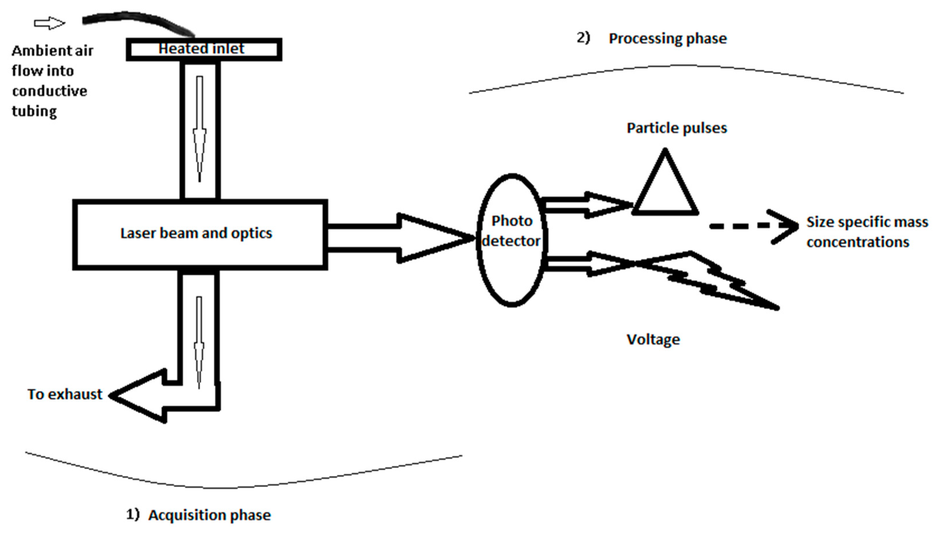
We used the TSI DustTrak™ DRX Aerosol Monitor Model 8533EP (TSI Inc, MN, USA) as the NRM to monitor PM in this study. The DRX is an attractive NRM because it combines two approaches to monitoring PM: (1) a photometer uses conventional light scattering technology to closely estimate particulate mass concentrations; and (2) a particle counter is used to measure particle size and number concentration by detecting the light scattered from individual particles [25]. The DRX is innovative in how it obtains and processes particle signals, and ultimately records mass concentrations of different PM size fractions (Figure 2). By individually sizing particles with an optical size larger than 1 µm diameter and calculating the mass of those particles, multiple mass fractions can be measured at the same time while improving the accuracy of reported mass concentration values [26].
The DRX was deployed at South Carolina’s only National Core Multipollutant Network (NCore) site within a manufacturer-provided environmental enclosure (DUSTTRAK Environmental Enclosure 8537) on a platform adjacent to the FEM sample inlet. Given concerns over humidity [27,28], the DRX was outfitted with a manufacturer-provided Heated Inlet Sample Conditioner (part number 801850) that effectively adjusts sampled air to a relative humidity (RH) to 50%. The humidity correction is intended to reduce potential measurement bias by maintaining a constant relative humidity level in the sample air stream before it enters the DRX optics chamber [29]. This Heated Inlet Sample Conditioner had an additional accessory, the Autozero Module (part number 801690) which was also attached to the DRX and programed to automatically re-zero the instrument every 24 h.

2.2. Data Collection, Management, and Preparation

FEM PM2.5 used in this study was collected with a Thermo Environmental Model 1405 F tapered element oscillating microbalance (TEOM) and reported at hourly intervals. Prior to reporting, data were verified by South Carolina Department of Health and Environmental Control (SC DHEC) personnel. NRM PM2.5 data were collected at one-minute intervals from the DRX and reported at hourly intervals to facilitate comparisons. Data Quality Assurance/Quality Control involved multiple steps designed to minimize instrumental errors. First, we only retained data if values of all PM size fractions were reported, the concentrations were >0 µg/m3, and all smaller size fraction concentration measures were equal or less than the larger size fractions’ concentration measures. Next, data were trimmed to retain the central 99% (0.5–99.5%) for the DRX in order to avoid potential skewing by data outliers. Finally, hourly data summaries were calculated for each size fraction if at least 80% of the one-minute data for a particular hour block were available.

2.3. Statistical Analyses

The aims of our statistical analyses were to conduct a field performance evaluation of our NRM and to construct a calibration curve for adjusting data based on observed differences with FEM. For evaluation, we use descriptive statistics, correlation coefficients, root mean square error (RMSE) and average bias (ab) to assess relationships between the DRX measurements and the FEM measurements. To construct our calibration curve, we employ a generalized additive model (GAM) to construct a non-linear function (i.e., penalized spline) that captures the relationship between FEM and NRM across our observed concentration range. Specifically, smooth functions (within GAMs) were developed using a combination of model selection and automatic smoothing parameter selection with penalized regression splines, which optimized the fit and made an effort to minimize the number of dimensions in the model [30]. Smoothing parameters were chosen through restricted maximum likelihood (REML) and, standard errors and corresponding confidence intervals were estimated using an unconditional Bayesian method [30].

2.4. Calibration Model

The framework of our generalized additive model can be expressed in following form:
Y i =   α   + s ( NRM _ PM i ) +   ε i
where Y is the hourly FEM referent PM2.5 concentration reported at time i during the co-located monitoring period, α is the intercept term, s is the smooth function representing NRM PM2.5 summarized measurements for hour i, and εi represents the error term, which is assumed to be normally distributed. Our model was fit using the ‘mgcv’ package in R: A Language and Environment for Statistical Computing [31].

3. Results

3.1. Co-Location Study

Ambient Conditions during Monitoring Period

Our co-location monitoring campaign began on 17 January 2018, and ended on 7 February 2018, giving us a 22 day (526 hr) observational period. Weather conditions during this time were generally cool, as average (standard deviation) temperatures were 9.2 (6.2) °C but ranged from −4.4 to 21.7 °C indicating modest variability. Relative humidity averaged 69.9 (25.6)% but ranged from 14.0 to 100% revealing that relatively dry to complete saturation (i.e., rain) events were experienced. Average (SD) wind speed was 1.6 (1.9) m/s and ranged from 0 to 9.3 m/s.

3.2. PM Data Summary and Evaluation

The focus of our co-location monitoring was to collect data that were suitable for comparison of our NRM to a FEM. As such, we first chose to implement EPA criteria [32] in selection of our comparison data and thus days in which 24 hr Federal Reference Method (FRM) measurements are below 3.0 µg/m3 were excluded. This criteria resulted in the dropping of 1 day (i.e., approximately 22 hrs) from our comparison period when the collocated FRM PM2.5 reported concentration was 2.2 µg/m3 (on 01/29/2018). However, we note the FRM data collection was every 3rd day during this study period and only available for 7 days (Table 1). As such, we chose to extend this criteria [32] to FEM data and dropped hourly FEM PM2.5 values less than or equal to 2.9 µg/m3. This criteria resulted in the additional exclusion of n = 98 h, where reported FEM TEOM values ranged from −3.6 to 2.9 µg/m3, giving us a final comparison period of 406 hrs in which PM conditions were deemed suitable for comparison [33].
During the sample period, the 1 hr average (SD) FEM PM2.5 concentration was 8.3 (4.6) µg/m3, indicating that air pollution levels were low to modest during our comparison. The 1 hr average (SD) NRM PM2.5 was 5.6 (3.5) µg/m3, indicating that our DRX, on average, reported lower levels than the FEM. Calculation of absolute bias (AB) confirms this difference at −2.54 µg/m3 during the comparison period (n = 406 h). The corresponding root mean square error (RMSE) was 2.55 µg/m3. Another aspect of interest in our evaluation was to determine how well our NRM tracked temporal changes in air quality reported by the FEM. To examine this, we plot these data over time to visualize agreement between the different measurement approaches (Figure 3). Here, we see that our NRM performed rather well at capturing the peaks and valleys in reported air quality. Correlation analysis confirms this, as we found strong positive agreement (R = 0.9) between hourly NRM and FEM data.
The final aspect of interest for our NRM evaluation is the reliability of our NRM to successfully capture data during a period of interest. Here, we found that the DRX performed very strongly, as we successfully monitored and retrieved data for nearly 526 hrs (31,528 min of data), indicating a capture rate of 100%; however, our data cleaning steps retained 99% of the one-minute data. Additional stringent criteria, such as removing hourly observations ≤ 2.9 µg/m3 (n = 98) and another 22 h with corresponding FRM measurement of 2.2 µg/m3, resulted in 406 total hours of data (77% of the original data: 406/526) which are used in subsequent analysis.

3.3. Statistical Calibration Model

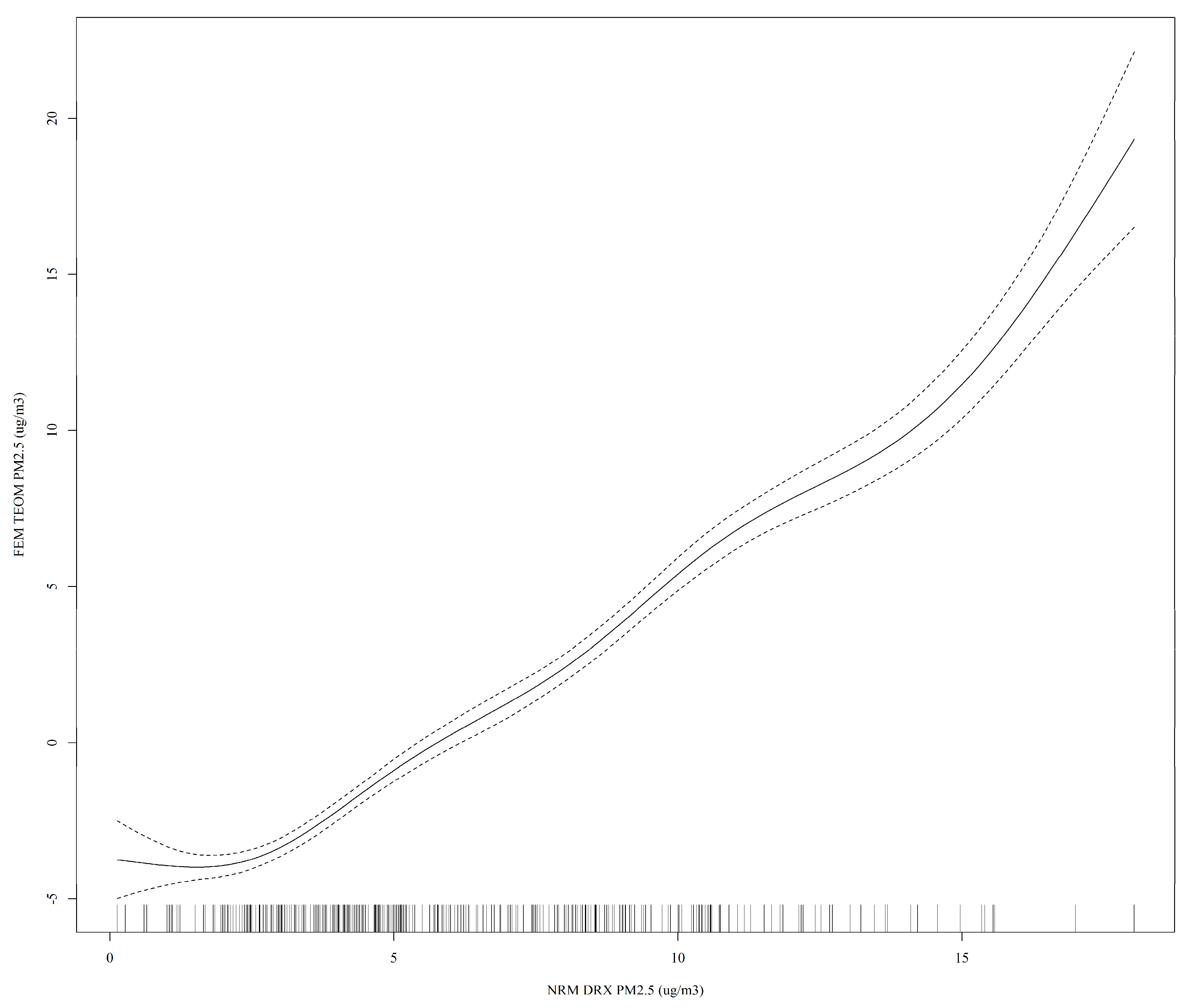
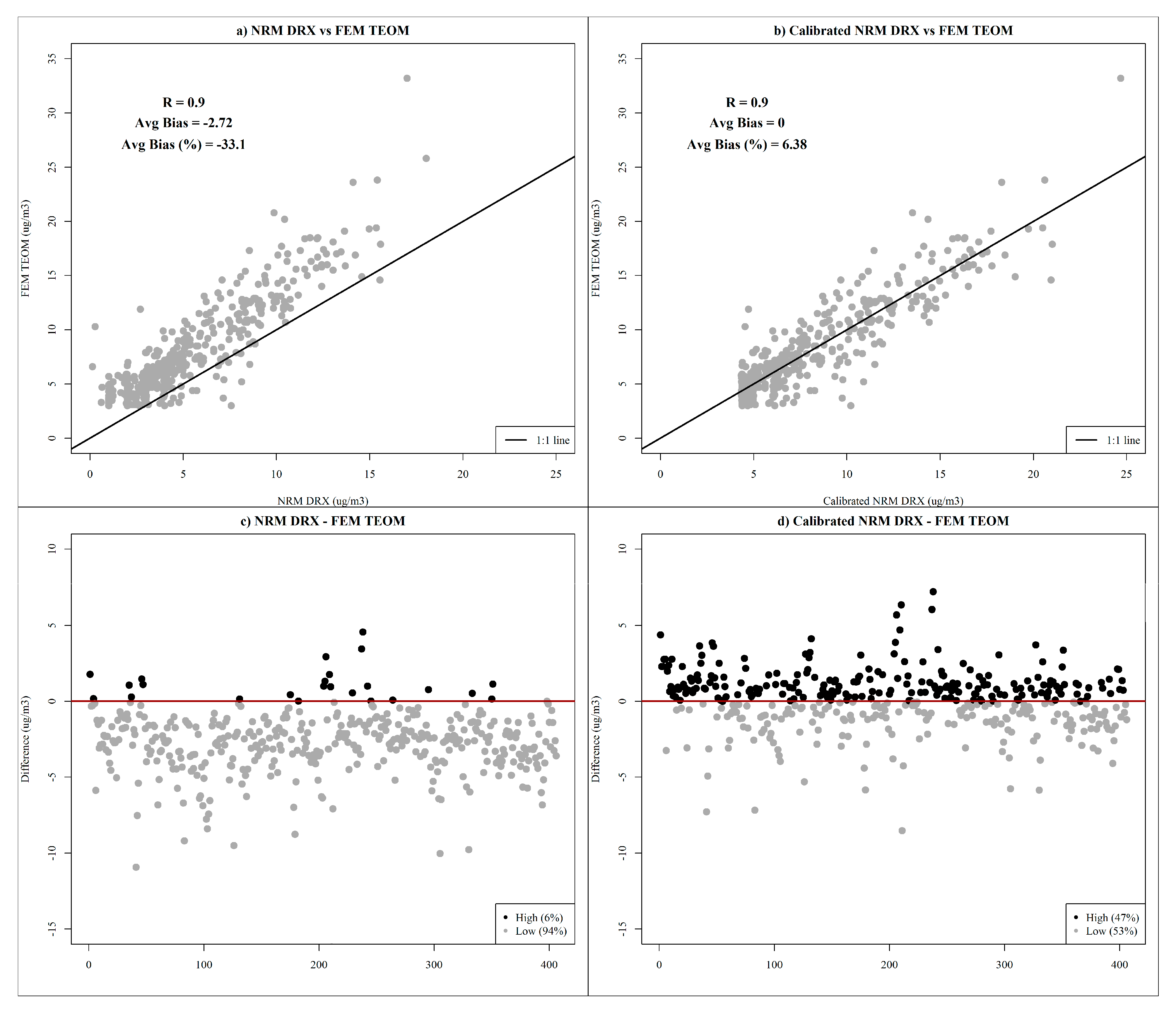
Results from our GAM fit found that our non-linear calibration curve (Figure 4) was able to explain 83% of the deviance (i.e., variability around the mean) of FEM reported 1 hr PM2.5 and had an R2 = 0.82. Application of our model fit to produce calibrated data shows that adjusted data retained the original correlation structure (R = 0.9) and that bias was successfully minimized, as average bias is reduced from 33% to 6% (Figure 5a,b). The average (SD) for the calibrated PM2.5 was 8.3 (4.1), with a range of 3–33 µg/m3. Examination of the calibration curve (Figure 4) reveals that the relationship with our response was non-linear, as we found areas of the data with strong agreement (~12 ug/m3) and areas where the ‘steepness’ of the curve varied (relatively low values, relatively high values). A resulting scatter plot of our calibrated data (superimposed over raw data) reveals the general positive shift in the data that our application of the model performs (Figure 5c,d).

4. Discussion

In this study, we aimed to illustrate how the development of statistical modeling tools can be used to improve reporting of particulate matter in studies that rely on non-reference monitoring (NRM) methodologies (e.g., low-cost sensors). The key finding from our study was that our statistical model can be applied to identify and remove non-linear trends in biases observed in data collected by our NRM monitor (Figure 5) and a FEM. Evaluations of raw NRM data identified a consistent negative bias (i.e., underreporting) in the DRX data that, if not accounted for, could lead to erroneous reporting in air quality studies. That said, raw DRX data tracked very well with reported FEM measures, indicating that raw data can be used to successfully monitor trends.
An important aspect of discussion for these data is to relate our findings to performance goals specified by EPA’s sensor evaluation guidelines [34]. To achieve this, we applied EPA formulations to our raw and calibrated NRM DRX data to improve understanding of how the resulting approach can be applied in community-based air quality studies. We found an overall bias error estimate of 33.1% for our raw NRM DRX data, a finding that implies that the raw DRX measurements are suitable for Education and Information only (TIER (or level) I, precision and bias error < 50%) [34]. However, when our calibration framework is employed, bias was reduced to 6.4%, indicating that calibrated NRM data can be used for hotspot identification and characterization (TIER II), and personal exposure monitoring (TIER IV). Guidelines for the precision and bias errors for TIERs II and IV are both < 30% [34]. We note that our findings may also be suitable to the requirements for supplemental monitoring (TIER III, precision and bias error < 20%). Overall, we find these results to be encouraging, as they demonstrate significant improvements in the reported data from our NRM and expand the potential applicability of the monitoring approach.
A detailed study by Rivas et al. identified several technical problems affecting the performance of the DRX including frequent artefact jumps, zero measurements and differences in actual ambient PM levels and DRX measurement records [35]. The authors recommended zero offset calibrations and the need to correct problematic data [35]. The field-based statistical calibration model illustrated in our study can be used to reduce bias and improve reporting of NRM data. There are multiple reasons why our NRM may have reported different values from the FEM TEOM method. First, we believe this may be partially explained by a loss of volatile and semi-volatile compounds during the heated inlet phase of air flow in the DRX monitoring schematic (Figure 2). This is postulated due to the simple fact that heat increases volatilization. This is consistent with other studies as a comparison study [36] in the United Kingdom observed differences in mass concentrations between a TEOM and a gravimetric sampler that were attributed to volatilization. Here, the authors noted that adding the calculated mass of ammonium nitrate significantly improved the mass concentration estimate and suggested that higher amounts of semi-volatile compounds tended to be associated with elevated PM levels [36]. Some of these semi-volatile compounds may have been lost at our sampling site. Other researchers have also pointed to the relationships between water and certain properties of PM components (e.g., inorganic or hygroscopic organic compounds) as important contributors to differences in mass concentrations [37,38].
Together, these factors must be considered and can complicate comparisons between instruments. Another possibility for our reporting of lower PM values is the potential for deposition to occur on the inlet tubing of the DRX. The DRX setup uses a seven inch slightly curved conductive tubing that connects to a 360o omni-directional sampling inlet and this may contribute to a longer than necessary sampling pathway. Furthermore, the NRM and TEOM operated at different flow rates during our study, a fact that impacted the amount of air pulled per volume and may have contributed to differences in reporting (Table 2). More specifically, the total flow rate for the DRX is 3.0 L/min, with 2.0 L/min serving as the measured sample volume and the remainder representing sheath flow. On the other hand, the TEOM operates at a total flow rate of 16.67 L/min, with a measured sample volume of 3.0 L/min and a bypass flow of 13.67 L/min. Additionally, both the NRM and the TEOM use heated inlets, hence air is sampled at approximately 50 °C, as opposed to being sampled at ambient temperature and pressure [29,36,39].

5. Limitations

As with all studies, our calibration framework is not without limitations. First, co-location studies can always benefit from increased durational periods as the breadth of conditions is an important factor to consider. As such, our campaign should only be viewed as an example because our period was relatively short and thus limits the interpretability of our results and applicability of the resulting calibration model. Ideally, co-location campaigns would capture the full range of conditions experienced in a potential air shed; however, we note that this may not always be feasible in community air quality studies. Another limitation that stems from our relatively short campaign is that our calibration curve may not be stable over the long term as we did not include data from other times of the year (e.g., summer) that may change the relationships between our reported data. A recent study highlighted the importance of re-evaluating model performance and new model development over time [40].
Another potential limitation of this study was that we did not adjust for meteorology in our calibration model. While inclusion of weather conditions may have improved model fit, we chose not to include weather conditions given the use of the heated inlet mechanism and that the air used to determine the mass concentrations was under relatively similar conditions. Finally, the scope of this work is limited to a particular type of sensor (the DRX) calibrated with data from in a single environment with low PM levels and for a limited period of time. As such, generalizing the specific results to other pollutants from different manufacturers and in different environments may be difficult. However, the concept of using GAMs to remove bias and improve data quality can be applied to other instruments and in a variety of environments. Such extended applications of this concept can improve the state of the science of low-cost air sensors and contribute to the further understanding of air pollution mixtures and their effects on human health.

6. Future Directions

Ultimately, our goal is to improve community outreach and awareness, and aid the development of community-based air pollution studies with accurate and interpretable data. As such, we plan to continue developing our calibration models with the intent of supporting future monitoring efforts in near port communities in Charleston, SC [41]. Our calibration framework may improve such efforts as high-quality data are required to document baseline measurements and can serve as a reference for potential future changes [42,43]. Additionally, gas- and particle-phase chemical analysis will be a major strength of such comparison studies in the future.

7. Conclusions

This study reveals that field-based statistical calibration models can be used to reduce bias and thus improve reporting of NRM in community air monitoring studies. This work also provides pertinent information needed for the voluntary performance evaluation program suggested by the US EPA. This work highlights the general usefulness of NRM technology for neighborhood-level air quality characterization. We also demonstrate that care is needed to interpret results. However, longer monitoring periods are recommended to understand neighborhood/community-level air quality.

Author Contributions

Conceptualization, J.P., S.R. and S.C.; methodology, J.P. and S.C.; software, J.P. and S.C.; validation, K.W. and S.R.: formal analysis, J.P. and S.C.; investigation, S.R. and A.M.; resources, J.P.; data curation, K.W. and S.C.; writing—original draft preparation, S.C.; writing—review and editing, A.M., C.P., K.W. and S.R.; visualization, S.C. and J.P.; supervision, J.P.; project administration, S.C.; funding acquisition, J.P. All authors have read and agreed to the published version of the manuscript.

Funding

Funding was provided by the Department of Public Health Sciences at the Medical University of South Carolina.

Acknowledgments

We would like to thank SC DHEC for providing access to the monitoring site and for the corresponding reference data.

Conflicts of Interest

The authors declare no conflict of interest.

References

  1. Dutta, P.; Aoki, P.M.; Kumar, N.; Mainwaring, A.; Myers, C.; Willett, W.; Woodruff, A. Common Sense: Participatory urban sensing using a network of handheld air quality monitors. In Proceedings of the 7th ACM Conference on Embedded Networked Sensor Systems; ACM: Berkeley, CA, USA, 2009; pp. 349–350. [Google Scholar]
  2. Miskell, G.; Salmond, J.A.; Williams, D.E. Use of a handheld low-cost sensor to explore the effect of urban design features on local-scale spatial and temporal air quality variability. Sci. Total Environ. 2018, 619, 480–490. [Google Scholar] [CrossRef] [PubMed]
  3. Popoola, O.A.; Carruthers, D.; Lad, C.; Bright, V.B.; Mead, M.I.; Stettler, M.E.; Saffell, J.R.; Jones, R.L. Use of networks of low cost air quality sensors to quantify air quality in urban settings. Atmos. Environ. 2018, 194, 58–70. [Google Scholar] [CrossRef]
  4. Krause, A.; Zhao, J.; Birmili, W. Low-cost sensors and indoor air quality: A test study in three residential homes in Berlin, Germany. Gefahrst. Reinhalt. Der Luft 2019, 79, 87–92. [Google Scholar]
  5. Jiao, W.; Hagler, G.; Williams, R.; Sharpe, R.; Brown, R.; Garver, D.; Judge, R.; Caudill, M.; Rickard, J.; Davis, M. Community Air Sensor Network (CAIRSENSE) project: Evaluation of low-cost sensor performance in a suburban environment in the southeastern United States. Atmos. Meas. Tech. 2016, 9, 5281–5292. [Google Scholar] [CrossRef] [Green Version]
  6. Fuller, C.H.; Patton, A.P.; Lane, K.; Laws, M.B.; Marden, A.; Carrasco, E.; Spengler, J.; Mwamburi, M.; Zamore, W.; Durant, J.L.; et al. A community participatory study of cardiovascular health and exposure to near-highway air pollution: Study design and methods. Rev. Environ. Health 2013, 28, 21–35. [Google Scholar] [CrossRef]
  7. Lane, K.J.; Levy, J.I.; Scammell, M.K.; Peters, J.L.; Patton, A.P.; Reisner, E.; Lowe, L.; Zamore, W.; Durant, J.L.; Brugge, D. Association of modeled long-term personal exposure to ultrafine particles with inflammatory and coagulation biomarkers. Environ. Int. 2016, 92–93, 173–182. [Google Scholar] [CrossRef] [Green Version]
  8. Kaufman, A.; Williams, R.; Barzyk, T.; Greenberg, M.; O’Shea, M.; Sheridan, P.; Hoang, A.; Ash, C.; Teitz, A.; Mustafa, M. A citizen science and government collaboration: Developing tools to facilitate community air monitoring. Environ. Justice 2017, 10, 51–61. [Google Scholar] [CrossRef]
  9. The Richmond Community Air Monitoring Program Chevron Richmond Refinery Fence Line and Community Air Monitoring Systems. Available online: http://www.fenceline.org/richmond/index.htm (accessed on 6 July 2016).
  10. Buonocore, J.J.; Lee, H.J.; Levy, J.I. The influence of traffic on air quality in an urban neighborhood: A community-university partnership. Am. J. Public Health 2009, 99, S629–S635. [Google Scholar] [CrossRef]
  11. EPA, U.S. Environmental Protection Agency. Planning and Implementing a Real-time Air Pollution Monitoring and Outreach Program for Your Community: The AirBeat Project of Roxbury, Massachusetts; EPA/625/R-02/012; Office of Research and Development, National Risk Management Research Laboratory: Cincinnati, OH, USA, 2002.
  12. EPA. Delivering Timely Air Quality, Traffic, and Weather Information to Your Community: The Paso Del Norte Environmental Monitoring Project; EPA/625/R-02/013; EPA: Cincinnati, OH, USA, 2003.
  13. Truax, C.; Hricko, A.; Gottlieb, R.; Tovar, J.; Betancourt, S.; Chien-Hale, M. Neighborhood Assessment Teams: Case Studies from Southern California and Instructions on Community Investigations of Traffic-Related Air Pollution; University of Southern California: Los Angeles, CA, USA, 2013. [Google Scholar]
  14. Chow, J.C. Measurement Methods to Determine Compliance with Ambient Air Quality Standards for Suspended Particles. J. Air Waste Manag. Assoc. 1995, 45, 320–382. [Google Scholar] [CrossRef] [Green Version]
  15. Castell, N.; Dauge, F.R.; Schneider, P.; Vogt, M.; Lerner, U.; Fishbain, B.; Broday, D.; Bartonova, A. Can commercial low-cost sensor platforms contribute to air quality monitoring and exposure estimates? Environ. Int. 2017, 99, 293–302. [Google Scholar] [CrossRef]
  16. Hagan, D.H.; Isaacman-VanWertz, G.; Franklin, J.P.; Wallace, L.M.; Kocar, B.D.; Heald, C.L.; Kroll, J.H. Calibration and assessment of electrochemical air quality sensors by co-location with regulatory-grade instruments. Atmos. Meas. Tech. 2018, 11, 315–328. [Google Scholar] [CrossRef] [Green Version]
  17. Holstius, D.M.; Pillarisetti, A.; Smith, K.; Seto, E. Field calibrations of a low-cost aerosol sensor at a regulatory monitoring site in California. Atmos. Meas. Tech. 2014, 7, 1121–1131. [Google Scholar] [CrossRef] [Green Version]
  18. Fishbain, B.; Lerner, U.; Castell, N.; Cole-Hunter, T.; Popoola, O.; Broday, D.M.; Iñiguez, T.M.; Nieuwenhuijsen, M.; Jovasevic-Stojanovic, M.; Topalovic, D.; et al. An evaluation tool kit of air quality micro-sensing units. Sci. Total Environ. 2017, 575, 639–648. [Google Scholar] [CrossRef] [PubMed]
  19. Mead, M.I.; Popoola, O.; Stewart, G.; Landshoff, P.; Calleja, M.; Hayes, M.; Baldovi, J.; McLeod, M.; Hodgson, T.; Dicks, J. The use of electrochemical sensors for monitoring urban air quality in low-cost, high-density networks. Atmos. Environ. 2013, 70, 186–203. [Google Scholar] [CrossRef] [Green Version]
  20. Piedrahita, R.; Xiang, Y.; Masson, N.; Ortega, J.; Collier, A.; Jiang, Y.; Li, K.; Dick, R.P.; Lv, Q.; Hannigan, M. The next generation of low-cost personal air quality sensors for quantitative exposure monitoring. Atmos. Meas. Tech. 2014, 7, 3325–3336. [Google Scholar] [CrossRef] [Green Version]
  21. Williams, D.E.; Henshaw, G.S.; Bart, M.; Laing, G.; Wagner, J.; Naisbitt, S.; Salmond, J.A. Validation of low-cost ozone measurement instruments suitable for use in an air-quality monitoring network. Meas. Sci. Technol. 2013, 24, 065803. [Google Scholar] [CrossRef]
  22. Williams, R.; Duvall, R.; Kilaru, V.; Hagler, G.; Hassinger, L.; Benedict, K.; Rice, J.; Kaufman, A.; Judge, R.; Pierce, G.; et al. Deliberating performance targets workshop: Potential paths for emerging PM2.5 and O3 air sensor progress. Atmos. Environ. X 2019, 2, 100031. [Google Scholar] [CrossRef]
  23. EPA, U. LIST OF DESIGNATED REFERENCE AND EQUIVALENT METHODS. Issue Date: 17 December 2016. Available online: https://www3.epa.gov/ttnamti1/files/ambient/criteria/AMTIC%20List%20Dec%202016-2.pdf (accessed on 25 October 2019).
  24. SC DHEC, 2018. Ambient Air Network Monitoring Plan: State of South Carolina Network Description and Ambient Air Network Monitoring Plan Calendar Year 2018; Quality, B.o.A., Ed.; SC DHEC: Columbia, SC, USA, 2017.
  25. Wang, X.; Chancellor, G.; Evenstad, J.; Farnsworth, J.E.; Hase, A.; Olson, G.M.; Sreenath, A.; Agarwal, J.K. A novel optical instrument for estimating size segregated aerosol mass concentration in real time. Aerosol Sci. Technol. 2009, 43, 939–950. [Google Scholar] [CrossRef]
  26. Naz, M.; Sulaiman, S.; Shukrullah, S.; Sagir, M. Investigation of Air Quality and Suspended Particulate Matter Inside and Outside of University Research Laboratories. Trends Appl. Sci. Res. 2014, 9, 43–53. [Google Scholar] [CrossRef]
  27. Day, D.E.; Malm, W.C.; Kreidenweis, S.M. Aerosol light scattering measurements as a function of relative humidity. J. Air Waste Manag. Assoc. 2000, 50, 710–716. [Google Scholar] [CrossRef] [Green Version]
  28. Day, D.E.; Malm, W.C. Aerosol light scattering measurements as a function of relative humidity: A comparison between measurements made at three different sites. Atmos. Environ. 2001, 35, 5169–5176. [Google Scholar] [CrossRef]
  29. TSI Inc. Heated Inlet Sample Conditioning Effects on Remote Dust Monitoring: Application Note EXPMN-008 (US). Available online: http://www.tsi.com/uploadedFiles/_Site_Root/Products/Literature/Application_Notes/EXPMN-008_Heated_Inlet_US-web.pdf (accessed on 29 November 2018).
  30. Wood, S. Generalized Additive Models; Chapman and Hall/CRC: New York, NY, USA, 2017. [Google Scholar] [CrossRef]
  31. R Core Team. R: A Language and Environment for Statistical Computing; R Foundation for Statistical Computing: Vienna, Austria, 2016; Available online: https://www.R-project.org/ (accessed on 22 July 2020).
  32. US EPA Quality Assurance Guidance Document. Quality Assurance Project Plan: PM2.5 Chemical Speciation Sampling at Trends, NCore, Supplemental and Tribal Sites. Available online: https://www3.epa.gov/ttnamti1/files/ambient/pm25/spec/CSN_QAPP_v120_05-2012.pdf (accessed on 7 April 2017).
  33. EPA. Ambient Air Quality Monitoring Program. In QA Handbook for Air Pollution Measurement Systems; EPA-454/B-13-003; EPA: Washington, DC, USA, 2013; Volume II, p. 348. [Google Scholar]
  34. Williams, R.; Kilaru, V.; Snyder, E.; Kaufman, A.; Dye, T.; Rutter, A.; Russell, A.; Hafner, H. Air Sensor Guidebook; EPA/600/R-14/159 (NTIS PB2015-100610); U.S. Environmental Protection Agency: Washington, DC, USA, 2014.
  35. Rivas, I.; Mazaheri, M.; Viana, M.; Moreno, T.; Clifford, S.; He, C.; Bischof, O.F.; Martins, V.; Reche, C.; Alastuey, A.; et al. Identification of technical problems affecting performance of DustTrak DRX aerosol monitors. Sci. Total Environ. 2017, 584–585, 849–855. [Google Scholar] [CrossRef] [PubMed] [Green Version]
  36. Charron, A.; Harrison, R.M.; Moorcroft, S.; Booker, J. Quantitative interpretation of divergence between PM10 and PM2.5 mass measurement by TEOM and gravimetric (Partisol) instruments. Atmos. Environ. 2004, 38, 415–423. [Google Scholar] [CrossRef]
  37. Price, M.; Bulpitt, S.; Meyer, M.B. A comparison of PM10 monitors at a Kerbside site in the northeast of England. Atmos. Environ. 2003, 37, 4425–4434. [Google Scholar] [CrossRef]
  38. Speer, R.E.; Edney, E.O.; Kleindienst, T.E. Impact of organic compounds on the concentrations of liquid water in ambient PM2.5. J. Aerosol Sci. 2003, 34, 63–77. [Google Scholar] [CrossRef]
  39. Meyer, M.B.; Patashnick, H.; Ambs, J.L.; Rupprecht, E. Development of a sample equilibration system for the TEOM continuous PM monitor. J. Air Waste Manag. Assoc. 2000, 50, 1345–1349. [Google Scholar] [CrossRef] [Green Version]
  40. Malings, C.; Tanzer, R.; Hauryliuk, A.; Kumar, S.P.; Zimmerman, N.; Kara, L.B.; Presto, A.A.; Subramanian, R. Development of a general calibration model and long-term performance evaluation of low-cost sensors for air pollutant gas monitoring. Atmos. Meas. Tech. 2019, 12, 903–920. [Google Scholar] [CrossRef] [Green Version]
  41. South Carolina Ports Authority Capital Plan. Available online: http://www.scspa.com/cargo/planned-improvements/capital-plan/ (accessed on 29 August 2019).
  42. Subramanian, R.; Ellis, A.; Torres-Delgado, E.; Tanzer, R.; Malings, C.; Rivera, F.; Morales, M.; Baumgardner, D.; Presto, A.; Mayol-Bracero, O.L. Air Quality in Puerto Rico in the Aftermath of Hurricane Maria: A Case Study on the Use of Lower Cost Air Quality Monitors. ACS Earth Space Chem. 2018, 2, 1179–1186. [Google Scholar] [CrossRef] [Green Version]
  43. Austin, E.; Coull, B.A.; Zanobetti, A.; Koutrakis, P. A framework to spatially cluster air pollution monitoring sites in US based on the PM2.5 composition. Environ. Int. 2013, 59, 244–254. [Google Scholar] [CrossRef]
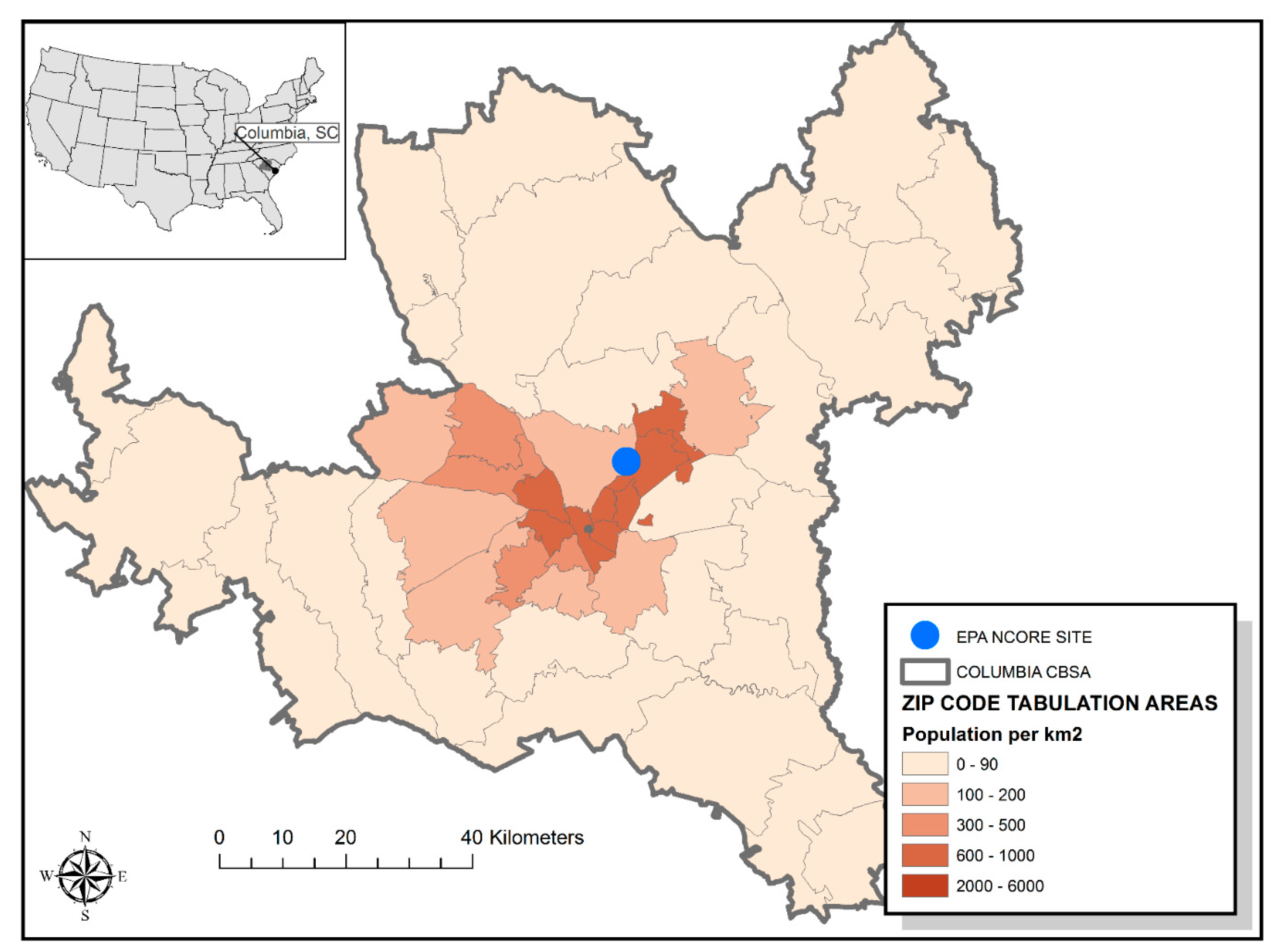
Figure 1. Map of study location depicting the study site within the Columbia core-based statistical area (CBSA). The CBSA represents an area with one or more counties anchored by an urban center of at least 10,000 people, together with adjacent counties that are socioeconomically associated with the urban center.
Atmosphere 11 00807 g001
Figure 2. Simple schematic illustrating measurement principle for the NRM DustTrak DRX. There are two main phases, namely the 1) acquisition and 2) processing phases.
Atmosphere 11 00807 g002
Figure 3. Timeseries of raw hourly NRM PM2.5 and FEM measurements.
Atmosphere 11 00807 g003
Figure 4. A smooth function estimated with a generalized additive model (GAM) reflecting the relationship (e.g., calibration curve) between our NRM monitor data (x-axis) and FEM data (y-axis). The solid line reflects the estimated response and the dash lines represent standard errors. Vertical lines on the horizontal axis indicate frequency of observations.
Atmosphere 11 00807 g004
Figure 5. Evaluation plots of our raw data (a) and generalized additive model (GAM)-based calibration data (b) for hourly PM2.5 for the NRM (DRX). (c) and (d) depict difference trends (DT) in hourly data points before and after applying the GAM-based calibration, respectively.
Atmosphere 11 00807 g005
Table 1. Summary statistics for measurements during co-located monitoring.
VariableInstrumentApproachPeriodnAvgSdMinMax
PM2.5 (µg/m3)DustTrak DRXNon-Reference1 hr4065.63.50.118
PM2.5 (µg/m3)Thermo Model 1405F TEOMFederal Equivalent1 hr4068.34.6333.2
PM2.5 (µg/m3)DustTrak DRXNon-Reference24 hr752.71.98.8
PM2.5 (µg/m3)Thermo Model 1405F TEOMFederal Equivalent24 hr77.13.7312.7
PM2.5 (µg/m3)GravimetricFederal Reference24 hr773.53.412.6
PM10 (µg/m3)Low VolumeFederal Reference24 hr711.23.94.515.9
Table 2. Characteristics of the DRX and FEM monitors used for the current study.
InstrumentDesignationMeasured Sample VolumeTotal FlowDifference
DustTrak DRX Aerosol Monitor 8533 Non-reference monitor (NRM) 2.0 L/min3.0 L/minSheath Flow Rate: 1 L/min
Thermo Model 1405 F Tapered element oscillating microbalance (TEOM) continuous PM monitorU.S. EPA PM-2.5 Equivalent Monitor3.0 L/min16.67 L/minBypass Flow Rate: 13.67 L/min