Atmospheric Simulations of Total Column CO₂ Mole Fractions from Global to Mesoscale within the Carbon Monitoring System Flux Inversion Framework

Abstract

Quantifying the uncertainty of inversion-derived ${\mathrm{CO}}_2$ surface fluxes and attributing the uncertainty to errors in either flux or atmospheric transport simulations continue to be challenges in the characterization of surface sources and sinks of carbon dioxide (${\mathrm{CO}}_2$). Despite recent studies inferring fluxes while using higher-resolution modeling systems, the utility of regional-scale models remains unclear when compared to existing coarse-resolution global systems. Here, we present an off-line coupling of the mesoscale Weather Research and Forecasting (WRF) model to optimized biogenic ${\mathrm{CO}}_2$ fluxes and mole fractions from the global Carbon Monitoring System inversion system (CMS-Flux). The coupling framework consists of methods to constrain the mass of ${\mathrm{CO}}_2$ introduced into WRF, effectively nesting our regional domain covering most of North America (except the northern half of Canada) within the CMS global model. We test the coupling by simulating Greenhouse gases Observing SATellite (GOSAT) column-averaged dry-air mole fractions (${\mathrm{XCO}}_2$) over North America for 2010. We find mean model-model differences in summer of ∼0.12 ppm, significantly lower than the original coupling scheme (from 0.5 to 1.5 ppm, depending on the boundary). While 85% of the ${\mathrm{XCO}}_2$ values are due to long-range transport from outside our North American domain, most of the model-model differences appear to be due to transport differences in the fraction of the troposphere below 850 hPa. Satellite data from GOSAT and tower and aircraft data are used to show that vertical transport above the Planetary Boundary Layer is responsible for significant model-model differences in the horizontal distribution of column ${\mathrm{XCO}}_2$ across North America.

1. Introduction

One of the persistent challenges in the study of the global carbon cycle is the quantification of the uncertainty in inferred biogenic carbon sources and sinks [1]. Contemporary solution methods include atmospheric inversions while using general circulation models and in situ or satellite observations of carbon dioxide (${\mathrm{CO}}_2$) to correct vegetation model or flux-derived estimates of these biogenic surface ${\mathrm{CO}}_2$ fluxes e.g., [2,3,4]. However, in spite of increasing sophistication in the optimization methods and observation systems, annual inverse fluxes vary widely at continental scales, e.g., from 0 to −1.5 PgC over North America [5]. Recent studies e.g., [6] assimilating in situ and satellite retrievals from the Orbiting Carbon Observatory (OCO)-2 NASA mission estimated the range of uncertainties between −0.5 to −1.6 PgC over North America. Contributions to this disagreement include poor representation of the heterogeneous land surface in relatively coarse general circulation models [7], as well as aggregation and atmospheric transport errors [8]. Inversions using column-averaged ${\mathrm{CO}}_2$ (${\mathrm{XCO}}_2$) show promise [9] as the ${\mathrm{XCO}}_2$ from satellites are presumed to be less susceptible to planetary boundary layer (PBL) atmospheric dynamics and heterogeneous surface fluxes [10,11]. Assimilating column-averaged ${\mathrm{CO}}_2$ observations is not without problems in terms of seasonal global coverage, interference from clouds, and large-scale transport errors [12]. The density of observations increases to unprecedented levels, requiring averaging or thinning techniques, so that global inverse models can ingest the large volume of data collected monthly [9]. An increase in atmospheric model resolution would potentially provide a better representation of the observed spatial variability in ${\mathrm{XCO}}_2$ over continents and allow for the assimilation of individual satellite retrievals [13], and may become even more important for the use of observations from geostationary satellites [14].

Regional models, which are capable of transporting ${\mathrm{CO}}_2$ as a trace gas, have been effectively used to simulate atmospheric ${\mathrm{CO}}_2$ gradients in regional studies [15,16] and generate footprints or back trajectories from observation locations to correct in-domain ${\mathrm{CO}}_2$ surface fluxes in comparison to existing agricultural inventories e.g., [7,17]. Several studies illustrated the value of regional models in exploring the near-field variability of ${\mathrm{CO}}_2$ fluxes and observed mole fractions, using a biogeochemical flux model coupled to a mesoscale atmospheric model and lateral boundary conditions modified from a global model [15,18,19]. However, these uses of regional models often assume that the large-scale boundary inflow is sufficiently known, so that fluxes within the regional domain dominate the observed variability e.g., [20,21]. To deal with total observable mole fractions of long-lived trace gases, background mole fractions (advected from outside the regional domain) must be dealt with carefully, e.g., [22]. Various strategies are in use; some are borrowed from the discipline of atmospheric chemistry research: constant concentrations [15], profiles from aircraft sampling, vertical transects derived from global models, and data over oceans [23], climatologies or average conditions from global models (see Tang et al. [24] for a review). For short campaigns, aircraft profile sampling can establish a curtain wall of boundary conditions in the upwind direction. Profile sampling schemes can be used to correct climatological conditions using monthly mean values. These climatologies or average conditions may be used for short-lived trace gases e.g., [25], but they do not fairly represent varying atmospheric circulation and transport. For long-lived trace gases, such as ${\mathrm{CO}}_2$, the vast majority of the molecules in any given volume is the result of long-range transport that originates outside the simulation domain.

Long-running regional ${\mathrm{CO}}_2$ inversion studies require time-varying, full-pro has been inversion-optimized mole fractions from global models, with and without adjustment to account for biases in the global model. For example, Göckede et al. [20] and Göckede et al. [21] used four-dimensional (4-D) lateral boundary conditions from the CarbonTracker global model [26] and verified the high sensitivity of regional inverse fluxes to the ${\mathrm{CO}}_2$ advected at the lateral boundaries. Bias-correcting offsets or adjustments to global model mole fractions have also been made based on comparisons to remote clean-air observations [27]. Lauvaux et al. [28] used a two-step approach, first adjusting the modeled mole fractions with local aircraft profiles and, second, optimizing them within the inversion system. Gourdji et al. [29] compared inversion results using an empirical data product that was derived from Pacific Ocean marine boundary layer observations and aircraft profiles [30,31] following Gerbig et al. [32] and described in Jeong et al. [33]. Ahmadov et al. [18] and Ahmadov et al. [19] incorporated ${\mathrm{CO}}_2$ initial and lateral boundary conditions from a global model (LMDZ; Peylin et al. [34]). Their lateral boundary conditions consisted of the results of a forward run of surface fluxes in LMDZ with an added constant offset to adjust the modeled ${\mathrm{CO}}_2$ mole fractions for general agreement with European in situ observations. He et al. [23] optimized boundary conditions using upper-air aircraft profile measurements (above 3000 m asl) while using global atmospheric mole fractions from a global inversion system and data-driven vertical transects.

In our study, we assume the optimized mole fractions from the global model can be used without further adjustment. We also choose the regional domain boundaries to be remote from the main area of interest in our study, and aim to conserve the mass of ${\mathrm{CO}}_2$ introduced at the boundaries of the simulation domain to be consistent between the global model and the regional model. This enables us to simulate column-averaged ${\mathrm{CO}}_2$ (${\mathrm{XCO}}_2$) in both global and regional models and compare to satellite-derived observations. This permits us to explore the impact in the regional model of surface ${\mathrm{CO}}_2$ fluxes optimized in the global model. To better understand the role of transport errors in our simulations, we also perform an ensemble of Weather Research and Forecasting-Chem (WRF-Chem) simulations while using identical fluxes from the NASA Carbon Monitoring System-Flux (CMS-Flux) inversion system but different transport realizations using the Stochastic Kinetic Backscatter Scheme (SKEBS; Berner et al. [35]). Do these fluxes produce equivalent results in the regional domain? How large are the differences in simulated ${\mathrm{XCO}}_2$ due to the use of different atmospheric transport models? Are the transport errors impairing our ability to infer surface sources and sinks? These are long-standing problems in ${\mathrm{CO}}_2$ inversion studies.

In our experiment, we introduce the optimized biogenic surface fluxes and posterior 4-D atmospheric mole fractions of ${\mathrm{CO}}_2$ from the Carbon Monitoring System (CMS-Flux; Liu et al. [36]) as initial and boundary conditions into the WRF-Chem regional model [37,38,39]. Here, we describe this framework for achieving our goal of conserving the mass of ${\mathrm{CO}}_2$ introduced in the regional model from the global model. In Section 2, we describe the global and regional models used in this experiment, the model coupling framework, and introduction to the methods for comparison to observation data. We present between-model consistency and comparisons to observations in Section 3. A discussion of the results follows in Section 4. Finally conclusions are presented in Section 5, including how the framework can be used to couple other global models to WRF.

2. Models and Methods

In this section, we provide an overview of the CMS-Flux inversion system, the customized WRF-Chem model, the coupling of the two modeling environments, the ensemble of WRF transport realizations, and the observations used to compare model results.

2.1. CMS-Flux Inversion System

The NASA CMS-Flux inversion system (http://cmsflux.jpl.nasa.gov) is described in detail in Liu et al. [36], an observing system simulation experiment (OSSE) to optimize biogenic fluxes using simulated Greenhouse gases Observing SATellite (GOSAT) ${\mathrm{XCO}}_2$ soundings [40]. The GOSAT Project (Japan Aerospace Exploration Agency, National Institute of Environmental Studies, and Ministry of the Environment) measures densities of ${\mathrm{CO}}_2$ and methane (${\mathrm{CH}}_4$) from space. The ${\mathrm{CO}}_2$ column abundances detected by the Thermal and Near Infrared Sensor for Carbon Observation-Fourier Transform Spectrometer (TANSO-FTS; Yakota et al. [40]) that we use in our experiment are processed using the NASA Atmospheric ${\mathrm{CO}}_2$ Observations from Space (ACOS) algorithm [41,42] for use as column-averaged ${\mathrm{XCO}}_2$ observations. The CMS-Flux inversion system uses the forward GEOS-Chem global chemical transport model [43,44] that is driven by meteorological fields from the NASA Goddard Earth Observing System, Version 5 (GEOS-5) data assimilation system [45]. ${\mathrm{CO}}_2$ is simulated as a passive tracer forced by emissions from fossil fuel, biomass burning, shipping and aviation, biogenic land, and ocean surface fluxes. The GEOS-Chem adjoint model [46] optimizes the biogenic surface fluxes and atmospheric ${\mathrm{CO}}_2$ mole fractions to be consistent with ${\mathrm{XCO}}_2$ from a satellite observing system [36,47]. The GEOS-Chem adjoint has been used to estimate carbon monoxide emissions [48,49] and to attribute direct ozone radiative forcing [50]. In our study, we couple all of the components of the CMS-Flux inversion system including the imposed surface fluxes and the optimized biogenic fluxes at the surface of the WRF model domain, but excluding two minor components of the fluxes (aircraft source and chemical sources). Atmospheric ${\mathrm{CO}}_2$ mole fractions from a coarse resolution global CMS-Flux inversion (horizontal resolution: $4^{\circ }$ latitude ×$5^{\circ }$ longitude; vertical resolution: 47 levels to 0.01 hPa) that assimilated GOSAT ${\mathrm{XCO}}_2$ for 2010 are coupled to the boundaries of the WRF simulation domain. Details of the imposed and prior surface ${\mathrm{CO}}_2$ fluxes can be found in Liu et al. [36] and they are summarized for North America in

Table 1. Surface fluxes for the North American domain in this study.

Surface Flux	Source	Temporal Resolution	Annual Budget (GtC yr${}^{-1}$)	Reference
Fossil Fuel	CDIAC	Hourly	1.77	Andres et al. [66]
Ocean	MITgcm, ECCO2,	3-Hourly	−0.25	Marshall et al. [67], Marshall et al. [68],
	Darwin project			Menemenlis et al. [69], Menemenlis et al. [70],
				Follows et al. [71],
				Dutkiewicz et al. [72],
				Follows and Dutkiewicz [73]
Biogenic	CMS-Flux, optimized	Monthly,	−1.07	Liu et al. [36],
	from CASA-GFED3	with imposed		van der Werf et al. [74], van der Werf et al. [75], van der Werf et al. [76],
		diurnal cycle		Olson and Randerson [77]
Biomass Burning	GFED3	Daily	0.11	van der Werf et al. [76],
				Mu et al. [78]
Biofuel	GFED3	Monthly	0.02	van der Werf et al. [76],
				Mu et al. [78]
Ship Bunker Fuel	ICOADS	Monthly	0.04	Nassar et al. [43], Nassar et al. [44]
* Aircraft and		Monthly	0.20	Nassar et al. [43]
* Chemical Source

* These non-surface sources are not included in the results that are presented in this work. When released as surface sources, they add ≤0.03 ppm to the ${\mathrm{XCO}}_2$ reported here.

. Figure A1 shows a schematic of the CMS-Flux system and the WRF-CMS interface for our experimental setup.

2.2. Weather Research and Forecasting with Chemistry Model (WRF-Chem)

The mesoscale model is WRF-Chem v3.6.1 [37,38,39,51] with the modification described in Lauvaux et al. [28] to transport greenhouse gases as passive tracers. Trace gas boundary conditions are provided from a global model at six-hourly intervals and surface fluxes introduced hourly. This work will describe (Section 2.4 below) the framework for introducing the boundary conditions from the global CMS-Flux model (using the GEOS-Chem atmospheric transport model to simulate ${\mathrm{CO}}_2$ mole fractions in the atmosphere) into the WRF domain in a manner designed to preserve the vertical distribution of ${\mathrm{CO}}_2$ at the WRF domain edges. Lauvaux et al. [28] used WRF-Chem for the forward transport model in an inversion for ${\mathrm{CO}}_2$ fluxes in the USA Upper Midwest region as part of the Mid Continent Intensive (MCI) campaign. This WRF-Chem implementation was also used in Lauvaux and Davis [13], who investigated the impact of introducing column-averaged ${\mathrm{XCO}}_2$ into regional inversions that typically use only ${\mathrm{CO}}_2$ observations measured in the planetary boundary layer.

In the experiment that is described here, the regional domain contains most of North America in a Lambert Conformal projection at 27 km horizontal resolution. The model has 50 levels up to 50 hPa with 20 levels in the lowest 1 km. The model meteorology is initialized every five days with six-hourly ERA-Interim [52] reanalysis at T255 horizontal resolution (∼80 km resolution over North America). Each meteorological re-initialization is started at a 12-h setback from the end of the previous five-day run. The first twelve hours of the new run are then discarded implying a discontinuity in ${\mathrm{CO}}_2$ transport necessary to re-initalize the meteorological conditions. We minimize the impact of the discontinuity by re-initalizing at night and by using the three-dimensional (3-D) ${\mathrm{CO}}_2$ mole fractions from the previous run to start the following one. We also employ the alternative lake surface temperature initialization as described in the WRF User Guide (Weather Research & Forecasting ARW Version 3 Modeling System User’s Guide, January 2015, pp. 3–26). Choices of the model physics parameterizations used in this experiment are documented in

Table 2. Weather Research and Forecasting (WRF) model physics parameterization choices.

Parameterization	Option Used	References
Longwave	Rapid Radiative Transfer Model	Mlawer et al. [79]
Shortwave	Dudhia	Dudhia [80]
PBL	Mellor-Yamada-Nakanishi-Niino Level 2.5	Nakanishi and Niino [81], Nakanishi and Niino [82]
Surface layer	Mellor-Yamada-Nakanishi-Niino	Nakanishi and Niino [81], Nakanishi and Niino [82]
Land Surface Model	Noah	Chen and Dudhia [83]
Cumulus	Kain-Fritsch	Kain [84]
Microphysics	WRF Single Moment 5-class	Hong et al. [85]

.

Carbon dioxide from surface fluxes from the CMS-Flux inversion (optimized biogenic ${\mathrm{CO}}_2$ fluxes and imposed ${\mathrm{CO}}_2$ surface fluxes from the ocean and emissions of fossil fuel, biomass burning, and ship bunker fuel; Table 1) are carried as individual tracers in WRF-Chem. Background ${\mathrm{CO}}_2$ mole fractions, supplied as boundary conditions from the CMS-Flux optimized mole fractions, are in a separate tracer. For analyses requiring total ${\mathrm{CO}}_2$ or ${\mathrm{XCO}}_2$, the surface flux tracers are summed after correcting for the presence of water vapor in GEOS-Chem to obtain dry air mole fractions, and added to the boundary condition tracer. This multiple-tracer strategy allows for the inspection of the separate tracers throughout the model integration. If total column values are required, then the region above the 50 hPa top of the WRF model is populated with the appropriate value from 50 hPa to 0.01 hPa from the global model. In this experiment, we do not include the non-surface fluxes of ${\mathrm{CO}}_2$ from the CMS-Flux inversion (aircraft source and chemical source; Table 1), but these are included in the boundary condition mole fractions from the global domain. A test, reducing these non-surface sources to surface emissions in the WRF domain, made, at most, a 0.03 ppm difference in the simulations of GOSAT ${\mathrm{XCO}}_2$.

The final preparation step for our experiment is the population of the WRF atmosphere with ${\mathrm{CO}}_2$ mole fractions from the CMS-Flux global model. It takes approximately a month’s integration in model time in order to distribute the contributions from the boundaries throughout the WRF atmosphere and completely remove the initial conditions from the simulation domain. For this experiment, we started the model integration in early December 2009, but begin all analyses in January 2010.

2.3. Ensemble Simulations (SKEBS)

An ensemble of ten perturbed transport realizations is performed to provide an assessment of transport model uncertainties. Perturbations of the meteorological driver data used to create initial and boundary conditions for WRF are generated by the Stochastic Kinetic Energy Backscattering scheme (SKEBS) [35]. Berner et al. [53] showed that a combination of a multiphysics scheme and perturbations from SKEBS represent more accurately transport model errors near the surface than perturbations alone. We selected a combination of model physics parameterizations to increase the spread of our ensemble. We used different combinations of Land Surface Models (LSMs) and planetary boundary layer (PBL) schemes in WRF, the main sources of variability in transport following Díaz-Isaac et al. [54]. We selected (1) Mellor-Yamada Nakanishi and Niino Level 2.5 (MYNN 2.5) PBL scheme with Noah LSM; (2) Mellor-Yamada-Janjic (MYJ) PBL scheme with RUC LSM; and, (3) Yonsei University (YSU) PBL scheme with five-layer thermal diffusion LSM. The SKEBS algorithm generates random perturbations to the meteorological initial and lateral boundary conditions. The SKEBS has been evaluated widely in the atmospheric ensemble modelling community while using similar parameter values to define the amplitude, sizes, and frequencies of the perturbations.

2.4. Mass Conserving Coupling Framework

In this experiment, we wish to compare simulated column-averaged ${\mathrm{CO}}_2$ from both the WRF execution and the CMS-Flux products with the ACOS GOSATv3.5 soundings [42] for North America. This requires that we ensure that the mass of ${\mathrm{CO}}_2$ introduced into the WRF domain from the CMS-Flux GEOS-Chem global model be conserved, both at the surface (fluxes) and the boundaries (atmospheric mole fractions) of the WRF model domain. The challenges for mass conservation include differences in model horizontal grid resolution, implied grid surface elevation, and vertical grid discretization. The strategy described here can also be used to couple the WRF regional model to other global models with a minimal amount of customization specific to the global model.

2.4.1. Mass Conservation of Surface Fluxes

We apply domain-wide scaling factors for each surface flux to conserve the mass of ${\mathrm{CO}}_2$ introduced into the domain by the surface fluxes. First, we create an exact map projection for translation from the low-resolution CMS-Flux GEOS-Chem $4^{\circ }$ × $5^{\circ }$ grid to the WRF 27 km grid (Figure A2 illustrates the domain extent of the WRF Lambert Conformal projection). Thanks to the higher resolution in WRF, the spatial mapping requires no interpolation or smoothing of the original CMS surface fluxes. We directly assign each WRF grid cell to the corresponding CMS pixel and compute monthly scaling factors for each surface flux component, as follows:

• Calculate the sum of the mass exchange in the global model grid cells assigned to the WRF domain.
• Calculate an initial domain-wide sum of mass exchange for the WRF grid cells using the assigned global model grid cells.
• Compute a domain-wide scaling factor as the ratio of the results of step 1 and step 2.
• Multiply the mass exchange assigned to each WRF grid cell by the domain-wide scaling factor.

These steps are repeated for each of the surface fluxes, including all the components of the CMS model, so that nearly-identical fluxes are used in WRF and CMS. The modification of the CMS total flux is due to minor misattribution along the coast lines, near water bodies, and due to non-perfect match between the two grids. The goal is to achieve equal total surface mass exchanges at the hourly resolution of the flux input into the WRF model domain. The component fluxes from CMS-Flux have temporal resolutions varying from hourly to monthly. The optimized biogenic flux is at monthly resolution, but with a 3-h diurnal cycle overlay with monthly net zero emission/uptake. We do not scale the diurnal cycle overlay. However, the surface fluxes in WRF have the same diurnal cycle. Only the scaling factors are being kept constant over a month. Most monthly scaling factors are in the range [1.0, 1.3] with the exception of some of the minor fluxes (biofuel and ship bunker fuel) with slightly larger scaling factors. The scaled surface fluxes are introduced into the WRF modeling system using the WRFCHEMI function of WRF-Chem. Realistic flux scaling results may also be achieved using a more sophisticated approach, such as the mass-conserving utilities within the NCAR Command Language (NCL) Earth System Modeling Framework (ESMF)), which would also retain the global model flux patterns, as well as preserving the domain mean.

2.4.2. Mass Conservation at the Domain Boundaries

The challenge in the case of the domain boundaries is not only the difference in horizontal resolution and grid type, but also the difference in vertical discretization schemes. WRF uses a terrain-following, hydrostatic-pressure vertical eta coordinate with a fixed model top. Because the top of the atmosphere in WRF is at 50 hPa, we used CMS mole fractions to complete the column values above 50 hPa in our study. The ${\mathrm{CO}}_2$ boundary mole fractions for our experiment are from a GEOS-Chem model with 47 hybrid-sigma layers corresponding to the GEOS-5 (MERRA) reduced vertical grid [45]. This grid is terrain-following from the surface up to ∼170 hPa, with fixed pressure levels from 170 hPa to the top of the model. Depending on the surface pressure and terrain, there may be nine layers below 1 km, compared to 20 layers below 1 km for our WRF domain. To approximate the vertical distribution of ${\mathrm{CO}}_2$ in the global model source in the WRF grid, we follow these steps for each WRF boundary grid cell:

• Compute an equivalent global model surface pressure for each WRF boundary grid cell using standard bi-linear interpolation (interpolating in two or more dimensions) using the four global model surface grid cells whose centers are closest in latitude and longitude to the WRF grid cell center.
• Compute the equivalent global model pressure column using this derived surface pressure and the standard vertical grid discretization for the global model, in this case the GEOS-5 hybrid sigma-pressure $ap$ and $bp$ parameters and algorithm for the 47-layer reduced vertical grid.
• Compute an equivalent WRF pressure column using this derived surface pressure and the $znu$ WRF vertical resolution discretization vector.
• Assign a source global model level for each receiving WRF model level in the WRF boundary grid (Figure 1). This is determined by the global model level edge pressures between which the derived WRF midpoint layer pressure falls. This computation is done in log space with the respective pressure columns in units of Pa.
• Use simple linear interpolation (if necessary) between global model levels to smooth out a poorly mixed flux signal. We used this technique for CMS-Flux GEOS-Chem where the first four or five model levels in WRF are sourced from the first GEOS-Chem level; this source layer often shows the immediate result of the surface flux as distinct from several well-mixed layers above the surface layer.
• The result of this transfer of vertical ${\mathrm{CO}}_2$ columns from the global model to the WRF boundary grid cells is introduced into WRF via the WRFCHEMBC functionality that is used for meteorological boundary conditions, similar to the approach of [18,19].

We use the GEOS-Chem surface pressure for two reasons. First, it is the mass in the GEOS-Chem column that we want to introduce into the WRF model domain and, second, it is not possible to match the surface pressures between the two models due to different horizontal grid resolutions, model grid surface elevations, and driver meteorology. To test the adequacy of this method, we compute pressure-weighted column-averaged ${\mathrm{XCO}}_2$ along the WRF boundaries, independently compute the same quantity from the global model up to 50 hPa, and compare the results. Figure 2 shows an example of this comparison for a day in early June 2010. The surface layer of the western and eastern boundaries of the WRF domain is predominantly ocean, where we do not expect significant model grid elevation or surface pressure differences. This is evident for this example date in Figure 2b. On the other hand, we do expect some differences in the southern and northern boundaries, particularly in mountainous areas (Figure 2a). Our algorithm produces model-model differences of column-averaged ${\mathrm{CO}}_2$ at the boundaries of less than 0.1 ppm on most of the boundaries and less than 0.3 ppm in the high-terrain regions of the northern boundary. We present a comparison of the mass-conserved coupling scheme to previous versions e.g., [28] in Section 3.1 to demonstrate the importance of mass conservation at the boundaries of the simulation for the use of column-integrated measurements.

2.5. Model Comparison to Observations

While a primary goal of this model coupling experiment is to compare WRF and CMS-Flux model-simulated ${\mathrm{XCO}}_2$ GOSAT soundings, it is comparisons to other observations that provide verification and insight into model behavior. In addition to the GOSAT ${\mathrm{XCO}}_2$, we compare to ${\mathrm{XCO}}_2$ from a Total Carbon Column Observing Network (TCCON) site for times of GOSAT overpasses. In order to understand the vertical distribution of ${\mathrm{CO}}_2$ and its relationship to column ${\mathrm{XCO}}_2$ values, we compared our simulated mole fractions to aircraft measurements and continuous tower measurements. We also compare model meteorological winds to observations from selected North American rawinsonde sites.

2.5.1. GOSAT XCO₂

We evaluated the WRF and CMS-Flux model-simulated ${\mathrm{XCO}}_2$ by comparison to to ACOSv3.5 LITE GOSAT soundings (Crisp et al. [41]) with more than 13,000 good quality soundings within the WRF North American domain during 2010. Reflected sunlight in three near-infrared bands are measured over a surface footprint of approximately 10 km in diameter at the nadir [55]. Nadir land and ocean glint observations were both used in our analysis.

The distribution of these soundings varies in space and time, with no coverage in ocean areas or north of ${60}^{\circ }$ N in winter. We follow the same sampling scheme in both WRF and CMS-Flux model ${\mathrm{CO}}_2$ mole fractions:

• Locate the nearest model grid cell in time and space to the GOSAT sounding.
• Isolate the column of ${\mathrm{CO}}_2$ at that grid cell, calculate the dry air mole fractions.
• Interpolate the simulated ${\mathrm{CO}}_2$ to the 20 pressure levels specified in the sounding’s ACOSv3.5 averaging kernel algorithm and a priori profile [42,56], as shown in the ACOS 3.5 User Guide.
• Apply the averaging kernel to the interpolated profile for the full column ${\mathrm{XCO}}_2$ or use the a priori profile pressure-level weights for partial column analysis.

Using the pressure-level weights versus the complete averaging kernel for the whole column yields results within a few tenths of a ppm for the full columns in our model atmospheres. For a priori profile pressure levels above 50 hPa, we use the CMS-Flux interpolated optimized mole fractions for both the WRF and CMS ${\mathrm{XCO}}_2$ computations. For ACOS GOSAT soundings with profile pressure levels below the model surface, we use the ${\mathrm{CO}}_2$ at the midpoint of the surface model layer.

2.5.2. Lamont TCCON XCO₂

The Total Carbon Column Observing Network (TCCON; Wunch et al. [57]) provides measurements of ${\mathrm{XCO}}_2$ from the earth’s surface at a global network of sites. Two TCCON sites within our North American domain were operating in 2010. The Park Falls site has significant drop-outs, especially in summer, so we choose the Lamont TCCON site ($36.6{}^{\circ }$ N, $97.49{}^{\circ }$ W) for comparison [58]. We average GOSAT soundings in a box of $6^{\circ }$ latitude and ${12}^{\circ }$ longitude centered at the Lamont site and match them to the TCCON data averaged for the hour of the GOSAT overpass of this regional box to include enough GOSAT soundings over each day in our analysis. This region corresponds to the US Upper Midwest with similar ecosystems and synoptic conditions, despite occasional frontal systems crossing the region. More advanced filtering methods have been developed to co-locate GOSAT and TCCON soundings [59], but we avoided using ${\mathrm{XCO}}_2$ fields from one of the two models to avoid biasing the selection process. We also computed hourly-averaged simulated ${\mathrm{XCO}}_2$ from the models for these GOSAT soundings in order to compare to both GOSAT and TCCON ${\mathrm{XCO}}_2$. During our period of comparison, summer of 2010, this region covers a large gradient of surface ${\mathrm{CO}}_2$ fluxes. Our goal is not to evaluate the GOSAT ${\mathrm{XCO}}_2$ relative to TCCON observations, but rather to illustrate how well the model-simulated ${\mathrm{XCO}}_2$ follow the general tendencies of the observations. More rigorous evaluation of the GOSAT ${\mathrm{XCO}}_2$ would require the use of coincidence criteria, as shown in Wunch et al. [60] or Basu et al. [61].

2.5.3. Horizontal Wind at Selected Rawinsonde Sites

We also make use of the NOAA archive of rawinsonde data (Schwartz and Govett [62]) for model comparisons to observed wind speed and direction at mandatory reporting levels. The goal in this case is to identify the possible causes of transport differences between models and observations. Comparisons of 00 UTC soundings (16–19 LST, depending on the site) are summarized to show annual and seasonal biases.

2.5.4. In Situ Tower and Aircraft CO₂ Observations

In order to evaluate the impact of transport differences between WRF and GEOS-Chem, and among the WRF ensemble members, we collected in situ ground-based data from the NOAA Tall Tower network [63] and from multiple aircraft profiles to diagnose differences in vertical ${\mathrm{CO}}_2$ distribution [64]. Continuous gas analyzers measure ${\mathrm{CO}}_2$ mole fractions using non-dispersive infrared (NDIR) absorption sensors (e.g., Licor Li-6200 series and Li-7000 analyzers) and Picarro Cavity Ring Down Spectrometers (CRDS) [65]. Calibration with high-accuracy gas cylinders and comparison to co-located discrete flask samples indicate measurement errors below 0.2 ppm. Discrete samples from the NOAA Aircraft Program are collected by the programmable 12-flask sampling systems at various altitudes (between 300 and 8000 m above ground level). ${\mathrm{CO}}_2$ mole fractions are measured by one of two nearly identical Measurement of Atmospheric Gases Influencing Climate Change (MAGICC) automated analytical systems. Measurement errors fall below 0.1 ppm, including possible sampling errors and storage biases.

3. Results

3.1. Evaluation of Transport Differences in Model-Simulated GOSAT XCO₂ Soundings

We compare the CMS-Flux and WRF ${\mathrm{XCO}}_2$ model simulations with GOSAT soundings without and with mass-conservation in WRF in

Table 3. Mean model residuals [ppm] relative to ACOSv3.5 GOSAT ${\mathrm{XCO}}_2$ for WRF without and with mass-conserved coupling schemes and CMS.

	Original Scheme	Mass-Conserved Scheme	Original CMS
Winter	0.624	0.294	0.269
Spring	0.492	0.071	0.031
Summer	1.412	0.569	0.015
Fall	0.768	0.226	−0.012

. The results from the mass-conserved coupling scheme in WRF reproduce more closely the original mismatches between CMS-Flux and GOSAT measurements. Mean mismatches in the original coupling scheme reach large values (up to 1.4 ppm) in Spring of 2010, and between 0.5 and 1 ppm during the other seasons. The histograms of the residuals are shown in Figure 3 revealing a similar range, positively-biased for all seasons. This first result demonstrates the decrease in the bias introduced in WRF by using a mass-conserved coupling scheme, whereas the original coupling artificially increases the amount of ${\mathrm{CO}}_2$ molecules in the atmosphere. We further compare ${\mathrm{XCO}}_2$ model simulations with each other in Figure 4 and with the GOSAT soundings in

Table 4. Model residuals [ppm] relative to ACOSv3.5 GOSAT ${\mathrm{XCO}}_2$. The span between the distribution quantiles Q3 and Q1 defines the interquartile range (IQR). IQRs for residuals of both models and all seasons are in the range [1.8, 1.9] ppm.

	Winter		Spring		Summer		Fall
	CMS	WRF	CMS	WRF	CMS	WRF	CMS	WRF
Maximum	5.91	5.51	6.52	7.45	6.58	7.31	9.42	9.03
Q3	1.25	0.97	1.28	1.09	1.18	1.31	0.96	0.79
Median	0.29	−0.00	0.38	0.16	0.26	0.34	0.07	−0.10
Mean	0.25	−0.04	0.31	0.11	0.26	0.38	−0.00	−0.15
Q1	−0.63	−0.91	−0.58	−0.79	−0.61	−0.52	−0.87	−1.01
Minimum	−18.00	−18.13	−19.21	−19.73	−7.95	−7.23	−9.64	−9.70
Soundings	1998		3113		3965		4305

. If we have reached our target of conserving ${\mathrm{CO}}_2$ mass entering the WRF domain from the CMS-Flux optimized ${\mathrm{CO}}_2$ surface fluxes and boundary conditions, then we expect the model-simulated ${\mathrm{XCO}}_2$ to be similar. Model–model differences can be related to transport from the boundaries into the WRF simulation domain (horizontal transit times from different driver meteorology and vertical mixing from boundary layer processes) or model resolution (heterogeneous surface characteristics). The seasonal mean model–model differences in ${\mathrm{XCO}}_2$ simulations are largest in winter (mean, −0.30 ppm; RMSD, 0.51 ppm) and smallest in summer (mean, 0.12 ppm; RMSD, 0.72 ppm). These seasonal distributions of differences are all sharply peaked around zero with a few large outliers (>5 ppm) in summer. Table 4 summarizes comparisons of model simulations to the GOSAT soundings. In spite of a few extreme outliers in winter and spring, the inner quartile ranges (IQRs) for both models relative to GOSAT are approximately 2 ppm, with nearly the same seasonal mean differences (CMS-Flux range [0.00, 0.31] ppm; WRF range [−0.04, 0.38] ppm). The median differences are slightly larger than the mean differences, except for the CMS-Flux simulations in summer and the WRF simulations in summer and fall. Although the model results are centered well with the GOSAT soundings, neither model produces simulations with the full range of values of the GOSAT ${\mathrm{XCO}}_2$. Because the WRF model is able to simulate the meteorological conditions at higher resolution, we might have expected more variability in the WRF simulations, as multiple GOSAT soundings assigned to a single grid cell in GEOS-Chem are represented by many grid cells in the higher resolution WRF grid. However, because surface fluxes remain at coarse resolution in both systems, we do not see any differences at this summary level. When considering the tails of the model-data residuals, only six individual GOSAT ${\mathrm{XCO}}_2$ soundings with model-GOSAT differences greater than 10 ppm were found; these soundings are all located over steep terrain in the western United States, hence most likely noise in the GOSAT measurements rather than due to the coarse resolution of the CMS-Flux system.

However, these general comparisons do not show differences in spatial coverage by season of the GOSAT ${\mathrm{XCO}}_2$ soundings or any spatio-temporal variations in model-model residuals. To address this, we aggregate the model-model differences to the CMS-Flux GEOS-Chem $4^{\circ }$ × $5^{\circ }$ grid to map the mean seasonal differences in each grid cell (Figure 5). We report in Figure 5 only those grid cells with more than 10 GOSAT soundings during each season shown. There are consistent small negative residuals in the WRF ${\mathrm{XCO}}_2$ simulations relative to CMS-Flux in most of the continent in winter and in the south and east in fall. The WRF–CMS-Flux differences are slightly positive in the northwest in fall. The pattern in spring is mixed. There are strong positive differences in the Pacific Northwest in summer. The underlying CMS-Flux optimized biogenic flux shows a very strong source of ${\mathrm{CO}}_2$ in the upper Pacific Northwest, and a correspondingly strong sink in the MidWest and East in July. These sources and sinks are evident in the WRF model layers closest to the surface, but not always in the CMS-Flux optimized mole fractions in the surface layers in the same locations. On some days, the surface layer flux contributions in the CMS-Flux ${\mathrm{XCO}}_2$ mole fractions are in grid cells adjacent to the emitting grid cells, which suggests some model–model differences in mixing and transport within the boundary layer. There are also sharp gradients in terrain height in this region that may contribute to the model differences, although this does not appear to be an issue in the Rocky Mountain region of the US West. In general, there is more variability in the spatial differences during the growing season. These maps also show how the spatial distribution of the GOSAT soundings changes by season. Note that there are no ocean soundings and no soundings in the high latitudes in winter. The examination of variances of the model-simulated soundings on this spatial scale show no clear differences between models, other than that there is less spatial variance in the models than in the GOSAT soundings.

Having documented the model–model differences in column-averaged ${\mathrm{XCO}}_2$ at seasonal scales, we next compare the distribution within the columns of the CMS-Flux and WRF ${\mathrm{XCO}}_2$ simulations. We expect to find the most differences in the active growing season, hence we focused on the comparison of summertime column estimates. We divide the columns into upper and lower portions, with the lower column corresponding to the three pressure levels closest to the surface in the ACOS algorithm, and with the upper column consisting of the remaining 17 levels. The ACOS averaging kernel pressure level weights specify ∼12.5% of the column-averaged value from the three pressure levels that are closest to the surface. The elevation above the surface of this split varies with terrain, but roughly corresponds to 850 hPa. As justification for this division, we highlight an example ${\mathrm{CO}}_2$ profile at the location of the LEF tall tower in Park Falls, Wisconsin, USA ($45.95{}^{\circ }$ N, $90.27{}^{\circ }$ W) at the time of a GOSAT overpass on 27 August 2010 (Figure 6). In this example, the ${\mathrm{XCO}}_2$ simulations from both the WRF total ${\mathrm{CO}}_2$ and the CMS-Flux optimized mole fractions agree with each other and with the ACOS GOSAT ${\mathrm{XCO}}_2$ (Figure 6a). The GOSAT ${\mathrm{XCO}}_2$ value is 385.526 ppm, with an uncertainty of 1.075 ppm; WRF and CMS-Flux simulated values are 385.706 and 385.245 ppm, respectively. We decompose the WRF total column ${\mathrm{XCO}}_2$ into contributions from the global model (light blue boundary conditions profile in Figure 6a) and the contributions of the flux tracers (Figure 6b). This is a location far from the boundaries of the WRF regional domain, so the boundary conditions profile is the result of long-range transport, not recent inflow. At this location and time, the flux contributions to the total ${\mathrm{CO}}_2$ profile are predominantly below 850 hPa. The minor ${\mathrm{CO}}_2$ fluxes (ocean, and combined biomass burning, biofuel, and ship bunker fuel emissions) contribute very little to the overall column value. The biogenic flux and the imposed fossil fuel emissions constitute almost all the flux portion of the column value. The transported boundary conditions account for more than 85% of the column-averaged ${\mathrm{CO}}_2$. For applications using total column ${\mathrm{CO}}_2$, it is important that this coupling of regional to global model be done correctly.

We illustrate the model–model differences for the simulated GOSAT ${\mathrm{XCO}}_2$ in summer using this ∼850 hPa division in Figure 7. Differences shown are for sub-column-averaged ${\mathrm{CO}}_2$ within the lower and upper portions of the column, computed as the sum of the interpolated mole fractions at each ACOS pressure level times the ACOS-provided weight at that pressure level. The lower portion of the column accounts for ∼50 ppm of the total column-averaged ${\mathrm{CO}}_2$. When comparing spatial patterns of differences of the sub-columns versus the total column in Figure 5c, we see that the WRF positive residual in the Pacific Northwest is the result of larger mole fractions in both upper and lower sub-columns. This is an area with a relatively low count of GOSAT soundings (Figure A3) and very large biogenic source flux. In the eastern half of North America, there is a dipole effect, with WRF simulations having lower mole fractions in the lower sub-column and higher values in the upper sub-column when compared to the CMS-Flux simulations. There are non-homogeneous patches of strong uptake in the biogenic flux in eastern North America in July, generally matching the spatial pattern in the lower sub-column. As a result, once re-scaled over the total column mole fractions (cf. Figure 7, lower panel), an additional 1 ppm is attributed to the lower part of the column over the West coast in WRF as compared to CMS-Flux, while the Great Lakes region and the Central part of North America shows a −0.5 to −1 ppm difference. The differences will reflect the attribution of the observed gradients to the north American surface fluxes as low levels interact with the surface while the upper part of the column is attributed to long-distance air masses. We note here that 1 ppm over the column and over the entire domain would correspond to an aggregated annual flux of 1 PgC over North America, or twice the natural sink over the continent. The upper sub-column pattern more closely resembles the total column pattern in Figure 5c. Model-model differences in other seasons are minimal in both parts of the column. The summer patterns illustrate that agreement of full column ${\mathrm{XCO}}_2$ simulations does not necessarily imply that the distribution of the ${\mathrm{CO}}_2$ is the same in the two models. This further suggests model–model differences in transport within the columns, possibly due to more vertical mixing in the CMS-Flux GEOS-Chem model. The CMS-Flux vertical profile in Figure 6a shows an example of this behavior.

3.2. Evaluation of Transport Differences in GOSAT XCO Soundings

The spatial differences between WRF and CMS-Flux ${\mathrm{XCO}}_2$ column mole fractions and ACOS GOSAT retrievals are shown in Figure 8, averaged over the summer of 2010. The two maps of model-data differences show similarities with positive values in the Central Great Plains and the coastal region of the Gulf of Mexico, and negative values over Canada and the West Coast of the US (cf. left and right upper panels in Figure 8). Differences are noisy, but, despite using different transport models, the overall model-data mismatches remain similar. Both models tend to over-estimate ${\mathrm{XCO}}_2$ column mole fractions in the North West of the US (region of Seattle, WA). To better understand the differences between the two transport models, we show in Figure 8 (lower panel) the differences between the two model-data mismatches (differences of the differences). The positive anomaly over the northwestern US dominates other regional differences, advected by the westerly flow following the Mid-latitudinal Jet Stream. The Jet advects this anomaly toward the central part of North America, generating a large mismatch of about 0.2 to 2 ppm between the two models. This anomaly is highly correlated with a large positive biogenic flux area in the CMS inverse fluxes, hence in both models but more pronounced in WRF, located over Seattle, WA. Looking at vertical profiles, this anomaly seems to be related to vertical mixing differences. GEOS-Chem, used in the CMS-Flux inversion system, tends to mix faster in the vertical, lifting CO${}_2$ molecules to higher altitudes where the wind speed is higher. We investigate the general behaviors of transport models in Section 3.4 using NOAA aircraft profiles across North America. WRF shows higher ${\mathrm{XCO}}_2$ values across the domain (0.57 ppm over summer) as compared to CMS (0.015 ppm), as shown in Table 3. This positive bias seems to be driven by the anomaly in the northwestern US.

3.3. Temporal Evaluation of Model-Simulated XCO₂ at the Lamont TCCON Site

A semi-independent comparison of column-averaged ${\mathrm{XCO}}_2$ for GOSAT and the model simulations is performed while using the ${\mathrm{XCO}}_2$ observations at the Lamont TCCON site. The calibration of ACOS GOSAT retrievals by comparison to TCCON measurements only accounts for long-term systematic errors, while our comparison focuses on short-term model-data differences. GOSAT passes near the Lamont TCCON site around 19 UTC. We select the GOSAT soundings near Lamont, as described in Section 2.5.2, average the ${\mathrm{XCO}}_2$ values by day and report them along with the 19 UTC hourly average of the TCCON observations. We present the weighted averages and standard deviations of both sets of observations in Figure 9a. The error bars in Figure 9a represent the root mean square uncertainties of the selected TCCON and GOSAT soundings included in the hourly averages. In the example shown for days in July and August 2010 when both observations are available, there are 1–21 good GOSAT soundings and 3–34 TCCON ${\mathrm{XCO}}_2$ observations during the 19 UTC overpass. Despite the presence of outliers in the early summer (around DOY 180–190), the daily average GOSAT and TCCON ${\mathrm{XCO}}_2$ soundings agree within 1–2 ppm, with discrepancies likely due to sampling and representation errors. The mean residuals of ACOS GOSAT, CMS-Flux, and WRF ${\mathrm{XCO}}_2$ relative to TCCON for this period are 0.088 ± 1.856 ppm, 0.868 ± 1.042 ppm, and 0.965 ± 0.981 ppm, respectively (Figure 9b). The residuals from the model simulations are generally, but not exclusively, positive and they are more similar to each other than to either of the observations. This implies that model transport differences are small when compared to other model-data differences at this time and location. The synoptic-scale variability in the summer atmospheric ${\mathrm{CO}}_2$ mole fractions is well represented during short-term events (e.g., near DOY 218). Despite the coarser resolution of the CMS-Flux mole fractions as compared to WRF, both models are able to capture the trend and variability observed by the Lamont TCCON site.

3.4. Vertical Transport Evaluation of Model-Simulated CO₂ at Several NOAA Aircraft Profile Sites

In order to understand the differences in total columns, we present an analysis of vertical profiles of ${\mathrm{CO}}_2$ mole fractions in Figure 10 focusing on two NOAA aircraft profile sites, one near West Branch, Iowa (WBI) in the central part of the US Corn Belt, and a second on the East Coast of the US near Charleston, South Carolina (SCA). Profiles were selected to represent both well-mixed conditions, during which the PBL top is well-defined and vertical ${\mathrm{CO}}_2$ gradients are close to zero (upper left and lower right panels), and near-neutral conditions when vertical mixing is driven by wind shear and thermals from the surface, responsible for non-zero ${\mathrm{CO}}_2$ gradients in the Lower Troposphere. Differences between WRF and CMS-Flux are observed in both the Free Troposphere and the PBL on 28 April 2010 (cf. Figure 10, upper left panel), with an under-estimation of the PBL height in WRF. The ensemble of WRF simulations is insufficient to explain the differences between the two transport models. On 29 November 2010 (cf. Figure 10, lower right panel), modeled ${\mathrm{CO}}_2$ mole fractions are consistent between the two models, but WRF captures correctly the near-surface gradient and values, independent of transport perturbations. For neutral cases ( e.g., Figure 10, upper middle panel), vertical gradients in ${\mathrm{CO}}_2$ mole fractions observed by the aircraft show a constant decrease until 3000 m above sea level. CMS-Flux shows a shallow and mixed PBL until 1000 m asl, while the ensemble of WRF simulations shows a similar gradient when compared to the observations but a wide range of values among transport ensemble members. A similar case is observed on 28 June 2010 (cf. Figure 10, lower left panel). The last two cases show an agreement between the two models, not matching the observed gradients nor the observed values in ${\mathrm{CO}}_2$ mole fractions. When considering the different cases shown here, we conclude here that models tend to agree in the Free Troposphere, but vary widely near the surface. The ensemble of transport realizations indicate a large spread among members in neutral conditions and a narrower range of vertical profiles during well-mixed conditions, despite the use of different physics schemes. In the Free Troposphere, the ensemble shows some variability due to variations in the origin of air masses. This result shows the importance of the transport of large-scale boundary conditions within the WRF domain, driven by uncertainties in the meteorological conditions over North America. These differences might also be due to differences in boundary conditions from the northern boundary, not fully reconcilable due to the steep terrain. Overall, we conclude that vertical mixing in the Lower Troposphere seems to drive the model-model ${\mathrm{CO}}_2$ differences, while the transport over long distances of large-scale ${\mathrm{CO}}_2$ air masses impacts ${\mathrm{CO}}_2$ mole fractions in the Free Troposphere. No clear improvement in the representation of observed vertical gradients in WRF as compared to the global CMS-Flux model is being observed over the vast majority of the profiles.

We further compare ${\mathrm{CO}}_2$ mole fractions from NOAA aircraft profiles to the two models (WRF and CMS) and to the contribution from the CMS boundary conditions alone within the WRF model in Figure 11. Total column ${\mathrm{XCO}}_2$ mole fractions are indicated for each vertical profile in order to understand the relationship between integrated mole fractions over the column and the vertical distribution of in situ mole fractions. For all four cases, WRF and CMS column ${\mathrm{XCO}}_2$ are within 1 ppm or less from each other, despite significant differences in the vertical distribution. Typically, mole fractions in the Free Troposphere remain similar. The corresponding GOSAT soundings are indicated with black stars, soundings collected nearby and within the hour. Only few profiles matched with GOSAT passing times. The accumulation of ${\mathrm{CO}}_2$ near the surface is a typical feature in CMS which might be problematic if tower data are being inverted, but not visible in satellite data. The surface fluxes in WRF impact the profiles up to 600 hPa (about 4000 m asl) as noted in the WBI profile on 1 July 2010 (cf. Figure 11, lower right panel). We also note that boundary conditions in WRF display a small vertical gradient near the surface, despite the long-range transport of air masses from the boundaries. This gradients implies that vertical gradients in CMS coupled to the boundaries can impact the vertical gradients in WRF, hence propagating vertical structures far into the WRF simulation domain. The largest differences are typically observed when surface signals are transported higher in the column, above the PBL (cf. Figure 11, lower right panel), advected by widely different horizontal mean wind. As shown in Lauvaux and Davis [13], vertical distribution matters, as it impacts the horizontal advection of surface signals, responsible for large spatial differences in the horizontal, as shown in Figure 8, lower panel).

3.5. Temporal Evaluation of Model-Simulated CO₂ at Several NOAA Tower Sites

We evaluated the modeled ${\mathrm{CO}}_2$ mole fractions at two NOAA towers: WBI sampling at 240 m agl and SCT sampling at 115 m agl, over a year, by showing the 31-day running mean Daily Daytime Averages (DDA) in Figure 12. These two locations correspond to the positive bias located in the US Midwest (WBI) and the negative bias (East Coast) diagnosed in WRF model residuals compared to CMS in Figure 8. At the surface, model-data differences agree with total ${\mathrm{XCO}}_2$ mole fraction differences during wintertime with lower mole fractions in WRF (cf. Figure 6), but tend to disagree in the summertime. The model-data differences are negative when compared to tower data in the summer whereas the total column values are positive. Positive model-data differences are observed over the PBL, between 500 and 600 hPa, as shown in Figure 11. We conclude here that model-data differences in the PBL do not reflect the overall differences in the column ${\mathrm{XCO}}_2$ mole fractions. When considering transport differences in the WRF ensemble, summertime model differences can be interpreted as transport differences at SCT, but not at WBI, with a larger drawdown in WRF. Spring and Fall seasons show little variability due to transport, while summer and winter show a larger spread in the ensemble. This result suggest that WRF ${\mathrm{CO}}_2$ mole fractions are primarily driven by large-scale conditions in shoulder seasons, reinforcing the importance of the coupling scheme when considering the annual carbon cycle. At SCT during the Fall season, WRF and CMS show large differences (about 2 ppm), despite the absence of fluxes from North America. We conclude here that long-range transport in the WRF domain differs from the CMS ${\mathrm{CO}}_2$ mole fractions. This analysis demonstrates the role of large-scale conditions and its transport within the regional simulation domain, esp. in Fall and Spring, and highlights the indirect relationship in model-data differences when comparing model-data residuals near the surface and in the ${\mathrm{XCO}}_2$ total column mole fractions.

3.6. Horizontal Mean Wind

We selected a group of rawinsonde sites (

Table 5. Rawinsonde sites used in comparison of 00 UTC modeled horizontal winds.

Site	WMO ID	Latitude (${}^{\circ }$N)	Longitude (${}^{\circ }$W)	Location Name
UIL	72797	47.95	124.55	Quillayut, WA, USA
OAK	72493	37.75	122.22	Oakland, CA, USA
NKX	72293	32.87	117.15	Miramar, CA, USA
YQD	71867	53.97	101.10	The Pas, MB, USA
BIS	72764	46,77	100.75	Bismarck, ND, USA
FWD	72249	32.80	97.30	Fort Worth, TX, USA
OAX	72558	41.32	96.37	Valley, NE, USA
SHV	72248	32.45	93.83	Shreveport, LA, USA
MPX	72649	44.83	93.55	Chanhassen, MN, USA
INL	72747	48.67	93.38	International Falls, MN, USA
DVN	74455	41.60	90.57	Davenport, IA, USA
JAN	72235	32.32	90.07	Jackson, MS, USA
BMX	72230	33.10	86.70	Shelby County, AL, USA
APX	72634	44.91	84.72	Gaylord, MI, USA
CHS	72208	32.90	80.03	Charleston, SC, USA
GYX	74389	41.60	70.25	Gray, ME, USA

; Figure 13), including west coast, east coast, Gulf Coast, and mid-continent North American sites for comparison of model and observed wind speed and wind direction at mandatory rawinsonde reporting levels. Our intent is to identify any regional distinctions in biases or variability that might help to explain the ${\mathrm{CO}}_2$ model-data differences. Each of these sites had more than 11 months of data for 00 UTC soundings in 2010 at the mandatory reporting levels of 925 hPa, 850 hPa, 500 hPa, and 250 hPa, which we used in our analysis. Continental mountain and high plains sites were not included, because they lack 925 hPa data, and cannot easily be compared with mandatory levels at lower elevation sites. Model locations were assigned as the nearest grid cell with similar surface height. For some coastal sites, the representative model sites were moved one grid cell toward the ocean to achieve this. In Figure 14, we show the annual mean wind speed bias at these sites from the WRF forward run (initialized with the ERA-Interim reanalysis) and the GEOS-5 reanalysis used by the CMS-Flux system. Recall that, although the WRF run is initialized with reanalysis data, it is free-running during each five-day run, and so may not conform to the reanalysis. Wind speed bias, RMSE, variance ratio, and correlation skill score ($\frac{Cov(model,obs)}{\sqrt{Var\left(model\right)Var\left(obs\right)}}$); von Storch and Zwiers [86]) are summarized in

Table 6. Model comparison to rawinsonde wind speed at mandatory reporting level 925 hPa, 00 UTC in 2010.

		WRF ERA-Interim				GEOS-Chem GEOS-5
Site	Count	Bias	RMSE	Correlation	Variance	Bias	RMSE	Correlation	Variance
		(ms${}^{-\mathbf{1}}$)	(ms${}^{-\mathbf{1}}$)	Skill	Ratio	(ms${}^{-\mathbf{1}}$)	(ms${}^{-\mathbf{1}}$)	Skill	Ratio
UIL	350	0.99	3.41	0.87	1.09	0.30	3.41	0.84	0.67
OAK	350	1.32	2.98	0.78	1.67	3.41	5.41	0.46	1.84
NKX	348	1.87	4.08	0.44	1.84	1.10	2.99	0.47	0.82
YQD	363	0.86	3.36	0.76	1.12	−1.24	2.67	0.86	0.68
BIS	349	0.71	3.04	0.73	1.02	−0.91	2.58	0.80	0.79
FWD	363	0.76	3.49	0.71	1.27	−1.21	3.06	0.75	0.79
OAX	364	1.59	4.30	0.71	1.13	−0.92	3.08	0.81	0.72
SHV	359	1.27	3.77	0.69	1.43	0.25	3.00	0.71	0.85
MPX	359	1.81	3.99	0.75	1.38	−0.65	3.35	0.71	0.79
INL	360	1.47	3.39	0.78	1.26	−1.01	3.14	0.73	0.70
DVN	357	1.44	4.10	0.76	1.25	−1.15	2.85	0.86	0.69
JAN	362	1.49	3.49	0.77	1.51	−0.04	2.45	0.80	0.85
BMX	362	1.21	3.32	0.78	1.37	−0.63	2.67	0.79	0.64
APX	358	2.44	4.15	0.75	1.87	−0.17	2.33	0.81	1.07
CHS	352	1.44	4.20	0.67	1.30	−0.58	2.47	0.84	0.72
GYX	362	2.63	5.54	0.71	1.54	−0.27	3.65	0.77	0.84

for mandatory reporting level 925 hPa. (See

Table A1. Model comparison to rawinsonde wind speed at mandatory reporting level 850 hPa, 00 UTC in 2010.

		WRF ERA-Interim				GEOS-Chem GEOS-5
Site	Count	Bias	RMSE	Correlation	Variance	Bias	RMSE	Correlation	Variance
		(ms${}^{-\mathbf{1}}$)	(ms${}^{-\mathbf{1}}$)	Skill	Ratio	(ms${}^{-\mathbf{1}}$)	(ms${}^{-\mathbf{1}}$)	Skill	Ratio
UIL	351	0.57	3.45	0.87	0.88	0.20	3.46	0.87	0.71
OAK	358	0.05	2.71	0.81	1.13	1.56	4.24	0.61	1.19
NKX	347	1.00	2.88	0.67	1.14	−0.16	2.65	0.64	0.84
YQD	363	0.53	3.77	0.74	1.10	−0.91	2.54	0.88	0.83
BIS	362	0.55	3.82	0.74	0.98	−1.18	2.99	0.86	0.81
FWD	363	0.29	3.95	0.70	1.05	−1.35	3.53	0.77	0.82
OAX	364	0.77	4.38	0.72	1.05	−1.37	3.43	0.83	0.83
SHV	359	0.64	3.83	0.71	1.12	−0.42	3.25	0.76	0.89
MPX	361	0.94	4.29	0.72	1.10	−1.31	3.91	0.75	0.79
INL	361	0.88	4.10	0.75	1.23	−1.20	3.68	0.76	0.75
DVN	358	0.99	4.60	0.72	1.21	−1.09	2.85	0.89	0.74
JAN	362	0.74	3.72	0.77	1.01	−0.78	2.98	0.84	0.71
BMX	363	0.75	3.55	0.79	1.17	−0.81	2.56	0.88	0.78
APX	358	1.66	4.63	0.74	1.27	−0.90	3.44	0.81	0.62
CHS	356	0.59	3.77	0.73	1.15	−1.16	2.91	0.84	0.86
GYX	362	0.97	5.48	0.69	1.17	−0.87	3.99	0.80	0.63

,

Table A2. Model comparison to rawinsonde wind speed at mandatory reporting level 500 hPa, 00 UTC in 2010.

		WRF ERA-Interim				GEOS-Chem GEOS-5
Site	Count	Bias	RMSE	Correlation	Variance	Bias	RMSE	Correlation	Variance
		(ms${}^{-\mathbf{1}}$)	(ms${}^{-\mathbf{1}}$)	Skill	Ratio	(ms${}^{-\mathbf{1}}$)	(ms${}^{-\mathbf{1}}$)	Skill	Ratio
UIL	350	−0.40	3.85	0.91	0.91	0.02	5.11	0.84	0.86
OAK	355	−0.16	3.61	0.93	0.97	−0.28	5.29	0.85	0.88
NKX	347	−0.54	3.43	0.93	0.96	−3.21	6.77	0.77	0.80
YQD	364	0.21	4.60	0.84	0.92	−0.80	3.34	0.92	0.80
BIS	361	0.66	5.03	0.82	1.03	−0.29	3.46	0.91	0.85
FWD	362	−0.42	4.14	0.92	1.10	−0.51	4.12	0.91	0.98
OAX	361	0.01	4.64	0.87	1.00	−0.61	4.16	0.89	0.83
SHV	355	−0.30	4.66	0.91	1.14	−0.95	4.47	0.91	0.90
MPX	359	0.36	5.27	0.83	0.94	−1.61	5.37	0.83	0.73
INL	360	0.31	5.32	0.82	1.02	−1.51	4.96	0.84	0.81
DVN	357	−0.15	4.88	0.87	1.04	−1.14	3.59	0.94	0.81
JAN	361	−0.16	4.39	0.92	0.95	−0.78	4.67	0.91	0.82
BMX	358	−0.22	4.39	0.92	0.95	−0.84	3.53	0.95	0.89
APX	359	0.78	5.09	0.86	0.99	−1.16	4.38	0.88	0.78
CHS	353	0.19	4.70	0.92	0.94	−1.03	4.17	0.94	0.76
GYX	361	0.06	5.60	0.85	1.02	−0.64	5.85	0.83	0.79

and

Table A3. Model comparison to rawinsonde wind speed at mandatory reporting level 250 hPa, 00 UTC in 2010.

		WRF ERA-Interim				GEOS-Chem GEOS-5
Site	Count	Bias	RMSE	Correlation	Variance	Bias	RMSE	Correlation	Variance
		(ms${}^{-\mathbf{1}}$)	(ms${}^{-\mathbf{1}}$)	Skill	Ratio	(ms${}^{-\mathbf{1}}$)	(ms${}^{-\mathbf{1}}$)	Skill	Ratio
UIL	345	−1.72	5.06	0.95	0.91	−0.40	7.87	0.85	0.80
OAK	354	0.64	4.52	0.95	0.98	−1.23	8.76	0.81	0.93
NKX	344	−0.53	5.03	0.94	1.11	−2.05	10.45	0.76	1.21
YQD	361	−0.68	5.97	0.90	0.91	−1.67	4.43	0.95	0.83
BIS	358	−0.37	7.14	0.88	0.95	−1.37	5.25	0.94	0.83
FWD	361	−0.39	5.80	0.94	0.95	−1.25	6.56	0.93	0.87
OAX	357	−0.55	6.21	0.91	0.94	−1.57	5.04	0.95	0.89
SHV	358	−0.79	6.11	0.95	0.89	−2.24	8.75	0.90	0.74
MPX	357	−0.23	6.77	0.90	0.91	−2.13	7.46	0.88	0.78
INL	360	0.01	7.12	0.88	0.96	−2.28	7.51	0.87	0.82
DVN	353	−0.09	7.25	0.89	0.97	−1.00	4.17	0.97	0.86
JAN	362	−0.10	6.17	0.95	0.86	−2.21	8.72	0.90	0.75
BMX	355	0.02	5.93	0.95	0.90	−1.72	5.97	0.95	0.87
APX	358	−0.54	7.36	0.88	0.94	−2.34	6.23	0.93	0.83
CHS	351	−0.05	5.94	0.96	0.93	−2.04	6.09	0.96	0.83
GYX	360	−1.76	8.78	0.86	0.86	−1.34	8.72	0.87	0.80

for results at other reporting levels). In general, coastal sites are difficult to simulate in both models, with seasonal differences that tend to cancel each other in WRF, but not in the GEOS-5 meteorology. With the exception of the coastal sites, WRF wind speed error is positively biased at the lower levels, but this bias largely disappears with height. Most notable is that GEOS-5 underestimates the wind speed for nearly all of this selection of sites at all levels. The WRF model overestimates wind speed variability by more than 10% at 925 hPa and 850 hPa, but slightly underestimates variability at higher mandatory levels. The GEOS-5 analysis consistently underestimates variability at all levels. Both models’ correlation skill scores improve with height, as expected (Table 6 and Table A1, Table A2 and Table A3). WRF overestimates day-to-day variability, as shown by the variance ratio, in winds at lower levels, and it has a larger RMSE than GEOS-5 at lower, but not higher, levels. GEOS-5 underestimates day-to-day variability at all levels. Annual wind direction bias and RMSE, for both models at all sites and mandatory levels, are smaller than the number of degrees separating reportable wind directions (not shown). However, at the 925 hPa mandatory level, there are seasonal directional biases at many sites in summer and at west coast sites in all seasons (Figure 15). This directional bias may contribute to the summer boundary layer differences in ${\mathrm{XCO}}_2$ simulations between the two models. Based on these results, the potential improvement from finer resolution WRF simulations in the resolution of mesoscale features and vertical structure near the surface is not evident from our continental-scale evaluations. We discuss further in Section 4 the impact of potential biases in WRF near the surface and in GEOS-5 at upper levels.

4. Discussion

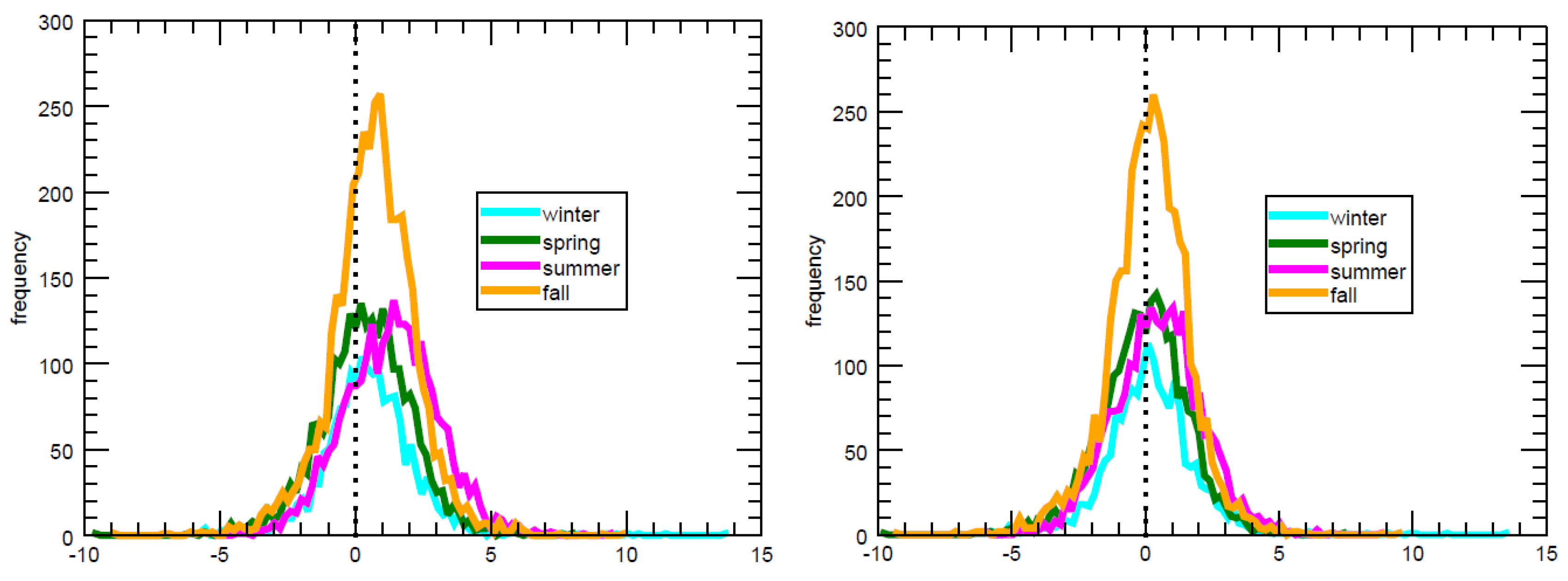
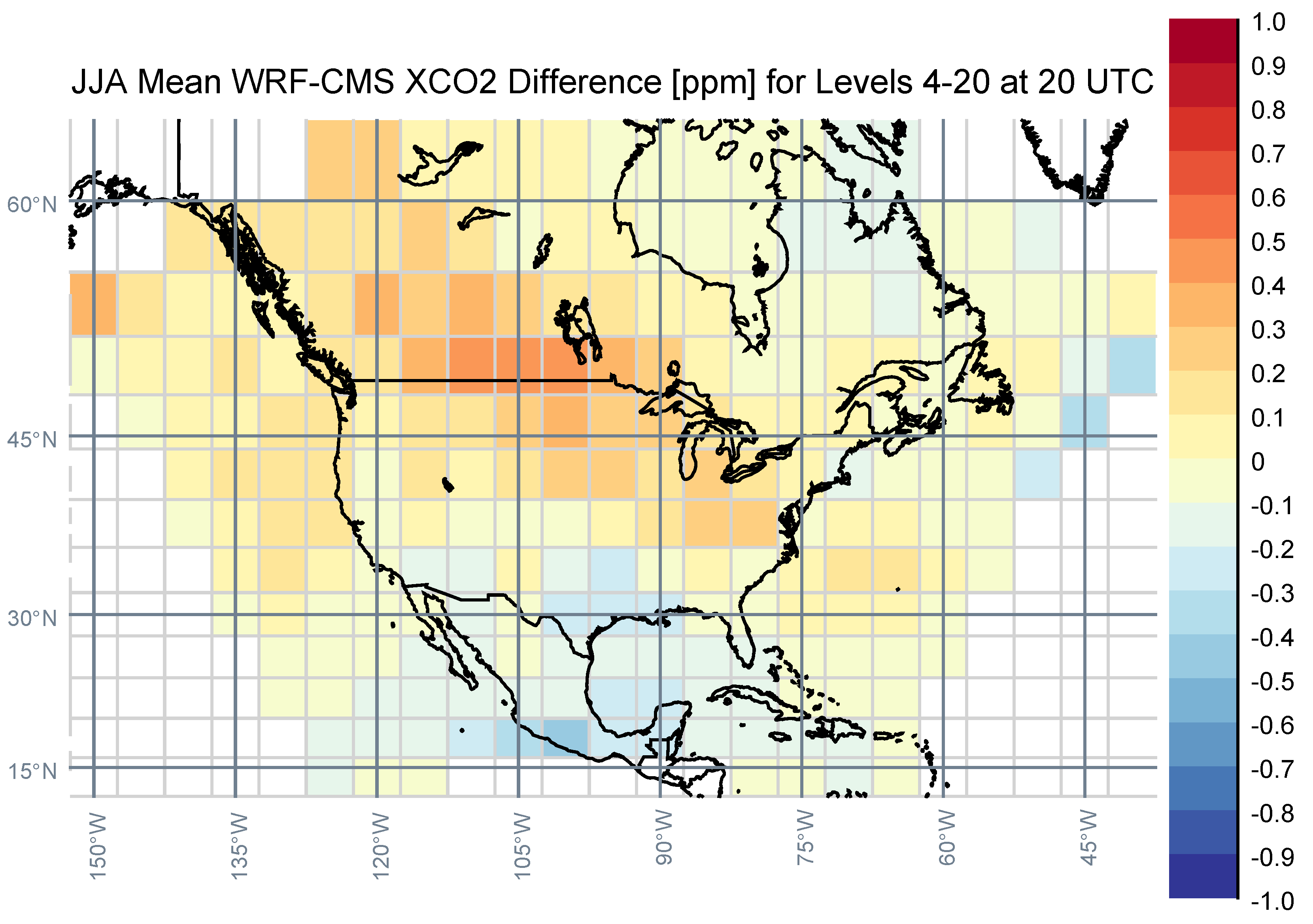
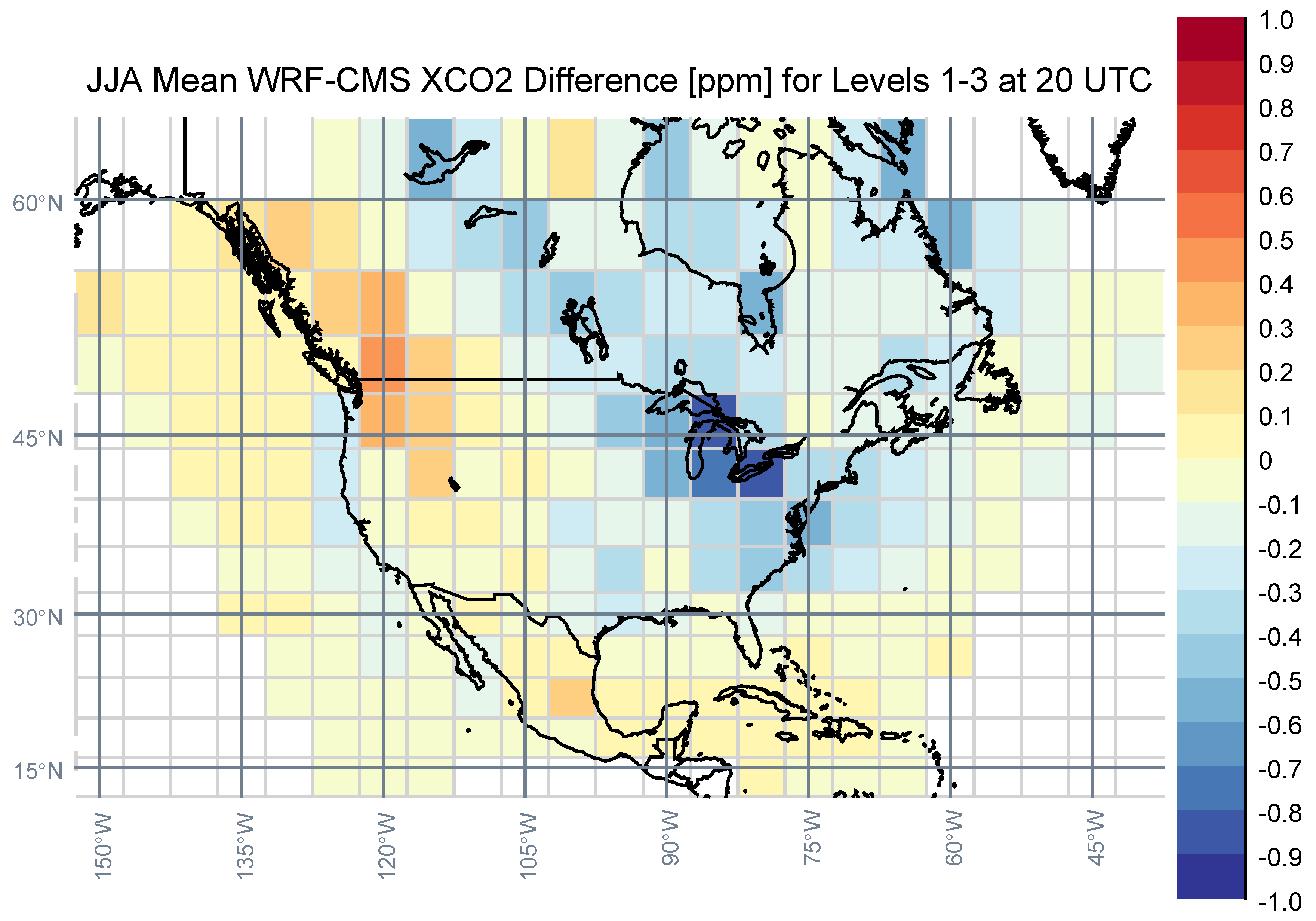
Based on the spatiotemporal distribution of GOSAT ${\mathrm{XCO}}_2$ soundings, there is very good agreement between the two modeling systems and GOSAT in the gross seasonal comparisons, well within the uncertainty of the individual GOSAT retrievals (0.5–2.00 ppm, reported with each sounding). Our primary goal of this framework is to control the ${\mathrm{CO}}_2$ mole fractions introduced into the WRF domain to be as close as possible to the mole fractions from the global model. By scaling the surface fluxes and constraining the mole fractions in the flow at the boundary walls, we have approached this goal of mass conservation. The largest spatiotemporal differences in ${\mathrm{XCO}}_2$ shown in this experiment appear to be due to the model–model differences in transport of the anomalous July biogenic source in the continental northwest and offsetting sinks in the midwest and east in the optimized CMS-Flux biogenic fluxes. However, the very small differences in simulated ${\mathrm{XCO}}_2$ values mask larger differences within the columns. For example, we can see model-model differences in the transport of the surface flux anomaly in the Pacific Northwest in summer, both within and above the boundary layer (Figure 7). Apparent model differences in vertical mixing within the boundary layer in summer in the eastern part of North America result in lower values within the boundary layer (<850 hPa, −0.5 to +0.1 ppm) and higher values above the boundary layer (>850 hPa, by +0.1 to +0.5 ppm) in the mesoscale model compared to the global model. We know that this configuration of WRF-Chem lacks convective mass transport of the ${\mathrm{CO}}_2$ tracers. This will affect the vertical transport of ${\mathrm{CO}}_2$ into and out of the boundary layer. We also acknowledge here that diurnal variations in CMS surface fluxes are prescribed and they might not exactly match the meteorological conditions in WRF. A comparison of fluxes and PBL variations at shorter timescales is needed in future studies, and might be optimized in the inversion systems e.g., [23]. The CMS-Flux optimized ${\mathrm{CO}}_2$ mole fractions also show effects of recent fluxes in the layer closest to the surface, and then nearly homogeneous mixing in the next several model layers, as seen in the example profile in Figure 6a and Figure 11.

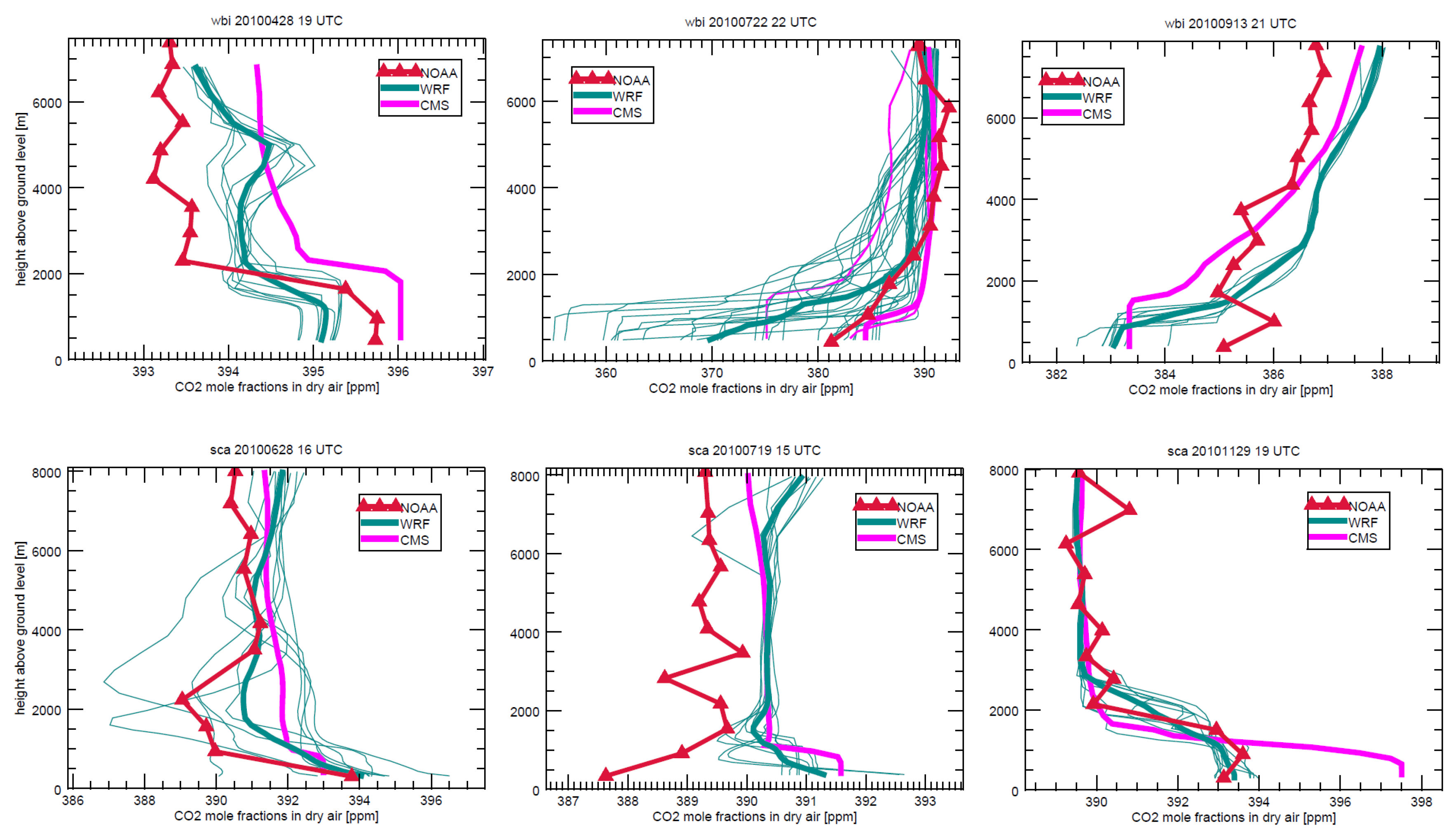
Comparison to in situ ${\mathrm{CO}}_2$ mole fractions collected during aircraft flights (NOAA aircraft program) showed that vertical air motion above the PBL top changes significantly the horizontal distribution of column ${\mathrm{XCO}}_2$. When comparing ${\mathrm{CO}}_2$ mole fraction biases at various tower locations (near the surface) to biases in column ${\mathrm{XCO}}_2$, seasonal and regional biases appeared to contradict each other, i.e., negative biases in Summer in ${\mathrm{CO}}_2$ while column ${\mathrm{XCO}}_2$ was positively biased. Detrainment of air out of the PBL, convection, and day-to-day PBL height variations lift up CO₂ molecules above the PBL, which are advected horizontally by fast-moving air masses in the Free Troposphere. A recent study showed the role of deep convection at Mid-latitudes by comparing two global models coupled to the same surface fluxes [87]. Their results suggest that the transport of continental surface fluxes by latitudinal atmospheric transport can greatly impact the distribution of ${\mathrm{CO}}_2$ mole fractions across the northern hemisphere. Similar to our results, they conclude that additional evaluation of vertical mixing is needed to reduce transport errors above the PBL, esp. by deep convection and other detrainment processes. The apparent agreement between models over the entire simulation domain was in fact hiding large differences in the vertical distribution, hence affecting the horizontal distribution of ${\mathrm{XCO}}_2$ at finer scales. The utility of aircraft data in our analysis explained some of the observed differences in column ${\mathrm{XCO}}_2$, not visible when comparing ${\mathrm{CO}}_2$ mole fractions at tower levels (within the PBL).

The ensemble of WRF realizations generated by perturbing the initial and boundary conditions and the model physics provided additional information on the impact of transport errors in the observed model–model and model-data differences. Seasonally, model-model differences are driven alternatively by the large-scale boundary inflow (Spring and Fall) or by the near-surface vertical mixing (Summer and Winter). Despite improving the coupling scheme with mass-conservation, differences remain between models, which are mostly due to differences in the transport of the CMS boundary conditions within the WRF simulation domain. Hence, model coupling is critical during off-seasons when signals from the surface are small, but when boundary conditions are affected by large-scale seasonal and synoptic variations. At the annual scale, transition seasons might cause the mis-attribution of large-scale inflow of ${\mathrm{CO}}_2$ into surface flux signals within the inverse system. Future studies will focus on the attribution of ${\mathrm{CO}}_2$ and ${\mathrm{XCO}}_2$ model-data residuals into surface and boundary contributions.

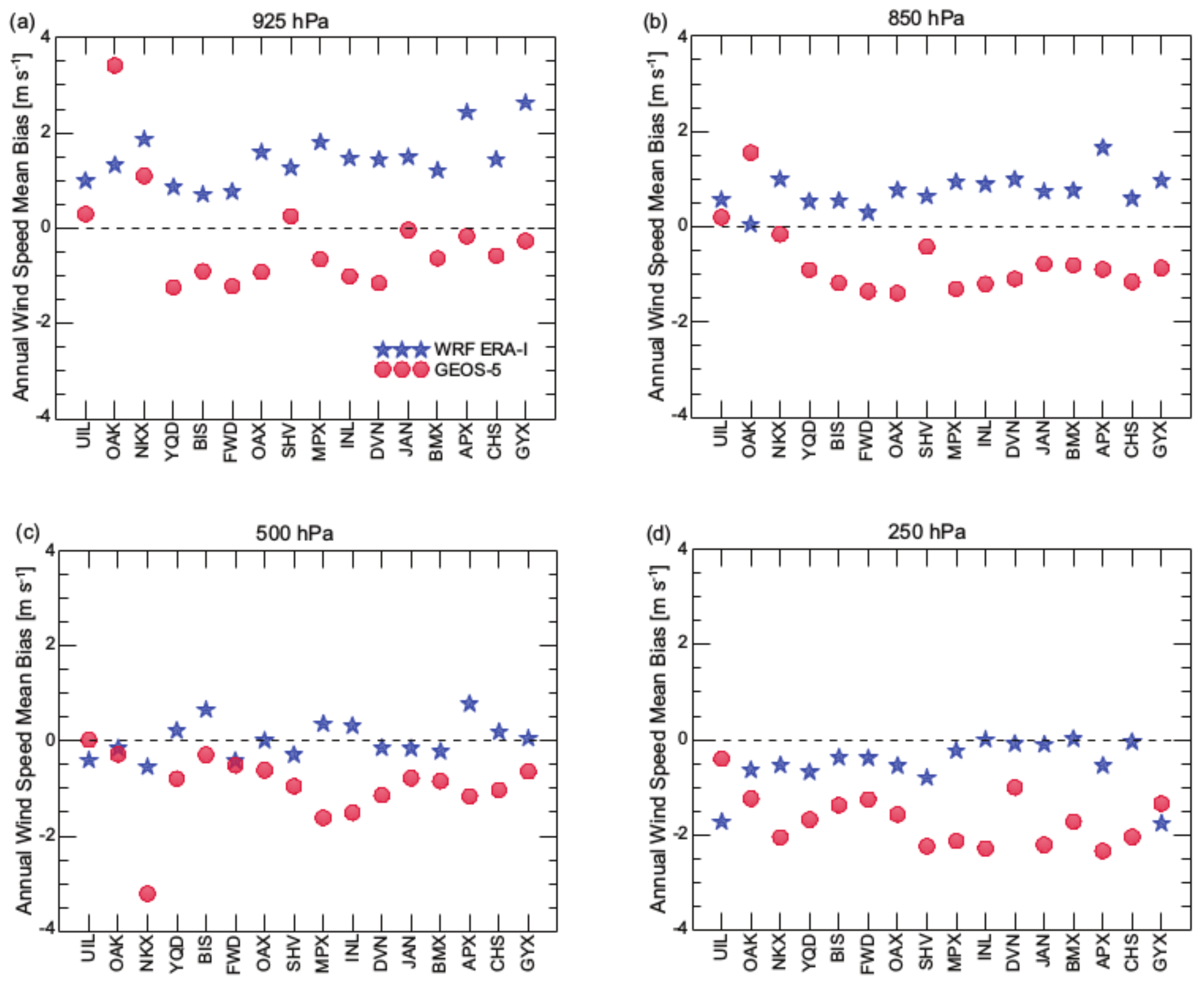
In this experiment, the meteorological evaluation of the WRF results was approximately comparable to the GEOS-Chem GEOS-5 results, and neither compared well in all respects with the rawinsonde observations. At the selected sites, the GEOS-5 winds were slow by up to 3 ms${}^{-1}$ at nearly all of the sites and mandatory levels that we used for comparison, while the WRF winds were closer to observations at higher levels. We had hoped to see better performance from the increased resolution, both horizontal and vertical, in WRF. Perhaps the horizontal resolution in WRF is still too coarse to take advantage of any truly mesoscale effects. We also did not assimilate meteorological observations into WRF; this was by design, as the primary focus of the experiment was to identify differences in transport of the ${\mathrm{CO}}_2$ originating from the CMS-Flux optimized biogenic fluxes. The WRF resolution, the assimilation of meteorological data in WRF, and changes to the boundary layer parameterizations within WRF could be tested to review the conclusions we see here. The two different re-analysis driver data used here might also cause differences in simulated ${\mathrm{XCO}}_2$ and ${\mathrm{CO}}_2$ mole fractions. No reconciliation was performed, because both models re-interpret driver data to a certain extent (through advection and diffusion schemes), acting as an additional layer of complexity. However, a comparison of ERA-Interim and GEOS-5 driver data would potentially bring additional information about transport differences and explain some of the differences noted here.

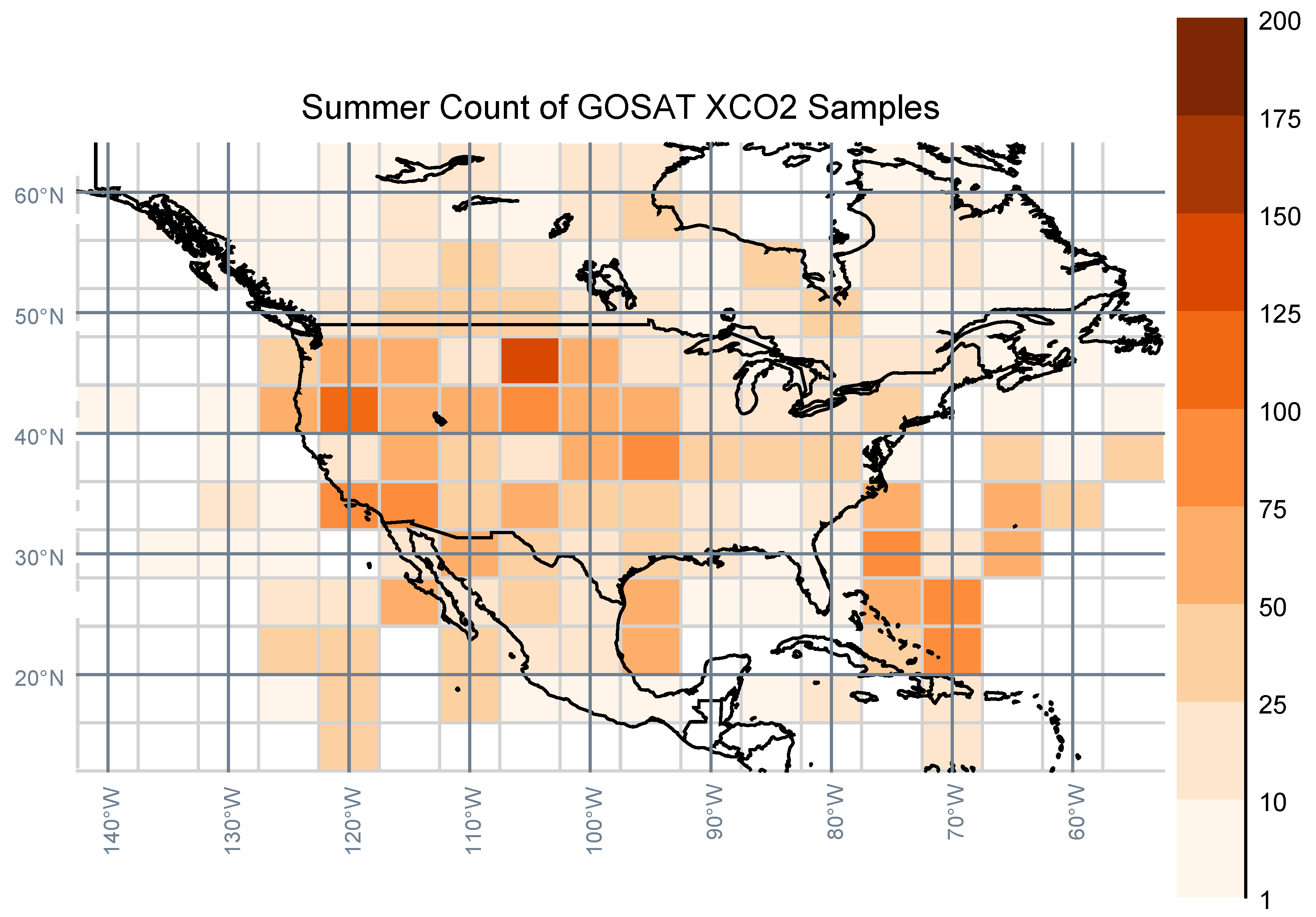
One of the main objectives of satellite ${\mathrm{XCO}}_2$ programs is to provide observations for assimilation into atmospheric inversions to improve the quality of inferred surface fluxes. GOSAT and other satellite missions ( e.g., OCO-2) provide good coverage of the North American domain in the summer, the season with the most biogenic activity. However, coverage in other seasons is limited, and must be supplemented with other ${\mathrm{CO}}_2$ observations, forcing the challenge of assimilating both column and surface observations in the same inversion. It is an interesting thought experiment to see what the model–model differences would be if we did have complete satellite sampling coverage over the course of a year. We sampled each model at its own horizontal grid resolution at the hour of the day with the most GOSAT ${\mathrm{XCO}}_2$ soundings (20 UTC), created simulated ${\mathrm{XCO}}_2$ from ${\mathrm{CO}}_2$ columns interpolated to the pressure levels commonly used in the ACOS algorithm, and examined model–model differences in the same way as we did with the simulated GOSAT soundings. We compared the differences for summer, the season with the best GOSAT spatial coverage (See Figure A4, Figure A5 and Figure A6). WRF values below 850 hPa are lower than the CMS-Flux values in the east, and WRF values are higher over most of the continent above 850 hPa. These results are reasonably consistent with the summer results that are shown in Figure 5 and Figure 7, which are conditioned on the spatiotemporal coverage of the GOSAT soundings. This is encouraging. While we will never have perfect coverage in every season with a satellite ${\mathrm{XCO}}_2$ product, the results presented here show that model-model differences do not appear to be overly dependent on the GOSAT sampling coverage. Future studies should also consider temporal correlations in the residuals when denser sampling is available ( e.g., OCO-2 or OCO-3) to examine the signatures of surface fluxes as compared to transport differences.

We have created a viable framework for comparing the transport of surface fluxes optimized in one model in another model. Theoretically, this allows for comparisons using different grid resolutions, meteorological drivers, and model parameterization options. In this experiment, we do see some differences between models in horizontal winds and boundary layer mixing, but see no clear advantage of the mesoscale model in the simulation of the satellite-derived ${\mathrm{XCO}}_2$. The framework does provide a computationally feasible laboratory for investigating other possible model configurations. Repeating the experiment in WRF with perturbations and using other configurations (boundary layer physics parameterizations) yield an ensemble of results that better establish an envelope of transport uncertainty for the CMS-Flux optimized biogenic flux solution. Additional sources of uncertainties, such as driver meteorological fields, assimilation of observed meteorology, or finer model resolution, might provide a more accurate range of transport simulations to establish an optimal configuration of the regional modeling system.

5. Conclusions

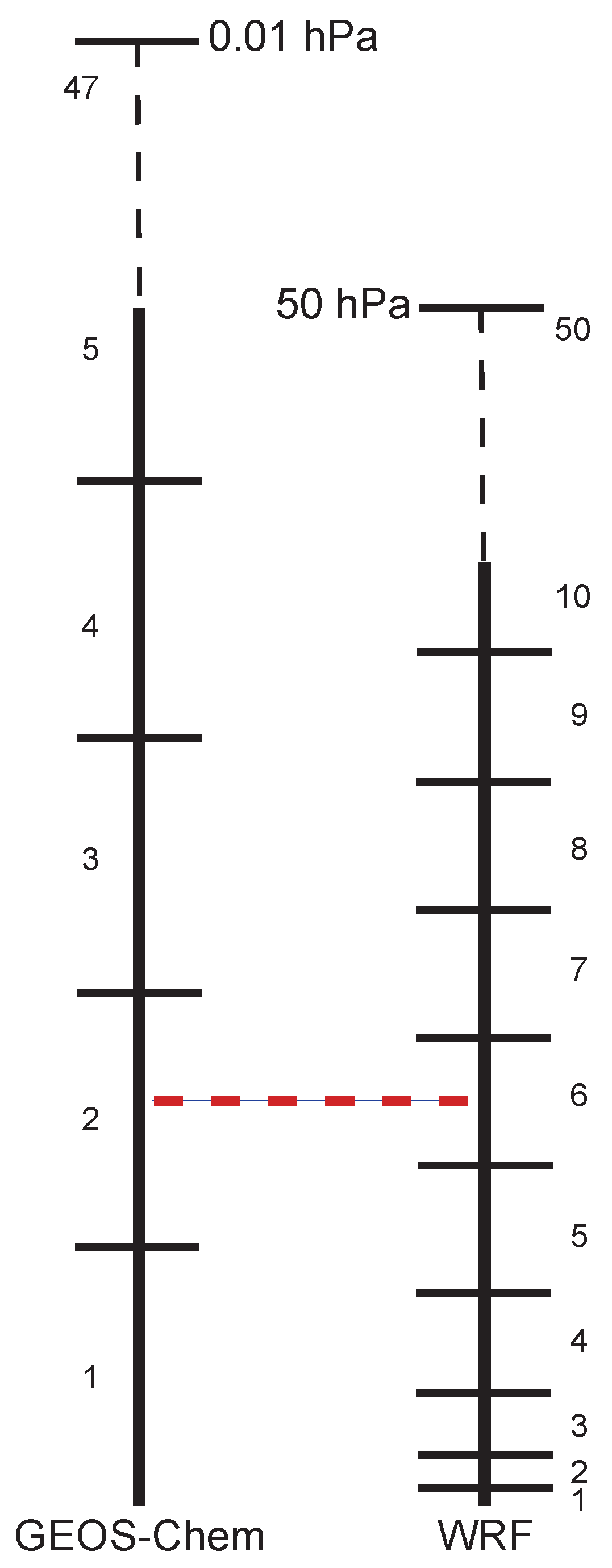
We have established a framework for effectively nesting a mesoscale model within a global model achieving approximate mass conservation of the trace gas ${\mathrm{CO}}_2$. The CMS-Flux and WRF simulated column-averaged GOSAT ${\mathrm{XCO}}_2$ samples are comparable within a few parts per million with some spatial differences, across all seasons and all geographic locations in the WRF North American domain. Our mass-conserved coupling scheme shows a significant improvement when evaluated against GOSAT data (0.1 to 0.5 ppm) as compared to traditional coupling schemes (0.5 to 1.5 ppm), more consistent with the model-data differences of the CMS-Flux inversion system. The models used here have very different horizontal and vertical resolutions and computational grids. The framework presented here makes it possible to follow the ${\mathrm{CO}}_2$ from surface fluxes optimized in a global model into a regional domain, allowing for the testing of various transport options.

Although simulations of entire columns agree when averaged over the domain between the models, noticeable vertical differences in the distribution of the ${\mathrm{CO}}_2$ within the column are shown by comparison to discrete flask samples from the NOAA aircraft program. These differences originate from vertical mixing in the PBL and in the transport of air masses from the boundaries into the WRF simulation domain. These differences, small when considering total column ${\mathrm{XCO}}_2$ from the models (less than 1 ppm on average) will affect the inverse sources and sinks across North America, attributing signals to the surface fluxes and the CMS-Flux boundaries differently for each model. Comparison to NOAA tower data revealed biases in Spring and Fall due to large-scale transport while Summer and Winter were affected by vertical mixing differences. A large fraction of the model differences in column ${\mathrm{XCO}}_2$ arose from the northwestern US and propagated into the simulation domain following the Mid-latitudinal Jet Stream. The differences are primarily explained by the vertical transport of ${\mathrm{CO}}_2$ molecules above the PBL top, where wind speed increases significantly, modifying the distribution of ${\mathrm{CO}}_2$ in the horizontal dimension. Unfortunately, both of the models show significant biases with respect to meteorological observations that vary with season. At the sites we examined, wind speeds are low in GEOS-5 in all seasons, especially at higher altitudes. WRF shows positive biases near the surface, while GEOS-Chem shows negative wind speed biases from the surface up to 250 hPa. There is the potential for significant transport bias with either modeling system, and in this experiment, WRF is not obviously better. Assimilating meteorological observations in WRF should reduce the wind bias in WRF, but the vertical mixing requires the calibration of the physical parameterizations to reduce vertical mixing differences across models.

References

1. Enting, I.G.; Rayner, P.J.; Ciais, P. Carbon cycle uncertainty in REgionalCarbon Cycle Assessment and Processes (RECCAP). Biogeosciences 2012, 9, 2889–2904. [Google Scholar] [CrossRef] [Green Version]
2. Gurney, K.R.; Law, R.M.; Denning, A.S.; Rayner, P.J.; Baker, D.; Bousquet, P.; Bruhwiler, L.; Chen, Y.; Ciais, P.; Fan, S.; et al. Towards robust regional estimates of CO2 sources and sinks using atmospheric transport models. Nature 2002, 415, 626–630. [Google Scholar] [CrossRef] [Green Version]
3. Baker, D.F.; Law, R.M.; Gurney, K.R.; Rayner, P.; Peylin, P.; Denning, A.S.; Bousquet, P.; Bruhwiler, L.; Chen, Y.H.; Ciais, P.; et al. TransCom3 inversion intercomparison: Impact of transport model errors on the interannual variability of regional CO2 fluxes, 1988–2003. Glob. Biogeochem. Cycles 2006, 20, GB1002. [Google Scholar] [CrossRef] [Green Version]
4. Maksyutov, S.; Takagi, H.; Valsala, V.K.; Saito, M.; Oda, T.; Saeki, T.; Belikov, D.A.; Saito, R.; Ito, A.; Yoshida, Y.; et al. Regional CO2 flux estimates for 2009–2011 based on GOSAT and ground-based CO2 observations. Atmos. Chem. Phys. 2013, 13, 9351–9373. [Google Scholar] [CrossRef] [Green Version]
5. Peylin, P.; Law, R.M.; Gurney, K.R.; Chevallier, F.; Jacobson, J.R.; Maki, T.; Niwa, Y.; Patra, P.K.; Peters, W.; Rayner, P.J.; et al. Global atmospheric carbon budget: Results from an ensemble of atmospheric CO2 inversions. Biogeosciences 2013, 10, 6699–6720. [Google Scholar] [CrossRef] [Green Version]
6. Crowell, S.; Baker, D.; Schuh, A.; Basu, S.; Jacobson, A.R.; Chevallier, F.; Liu, J.; Deng, F.; Feng, L.; McKain, K.; et al. The 2015–2016 carbon cycle as seen from OCO-2 and the global in situ network. Atmos. Chem. Phys. 2019, 19, 9797–9831. [Google Scholar] [CrossRef] [Green Version]
7. Schuh, A.E.; Denning, A.S.; Corbin, K.D.; Baker, I.T.; Uliasz, M.; Andrews, A.E.; Worthy, D.E.J. A regional high-resolution carbon flux inversion of North America for 2004. Biogeosciences 2010, 7, 1625–1644. [Google Scholar] [CrossRef] [Green Version]
8. Kaminski, T.; Rayner, P.J.; Heimann, M.; Enting, I.G. On aggregation errors in atmospheric transport inversions. J. Geophys. Res. Atmos. 2001, 106, 4703–4715. [Google Scholar] [CrossRef] [Green Version]
9. Liu, J.; Bowman, K.W.; Schimel, D.; Parazoo, N.C.; Jiang, Z.; Lee, M.; Bloom, A.A.; Wunch, D.; Frankenberg, C.; Sun, Y.; et al. Contrasting carbon cycle responses of the tropical continents to the 2015–2016 El Nino. Science 2017, 358, eaam5690. [Google Scholar] [CrossRef] [Green Version]
10. Rayner, P.J.; O’Brien, D.M. The utility of remotely sensed CO2 concentration data in surface source inversions. Geophys. Res. Lett. 2001, 28, 175–178. [Google Scholar] [CrossRef] [Green Version]
11. Keppel-Aleks, G.; Wennberg, P.O.; Schneider, T. Sources of variation of total column carbon dioxide. Atmos. Chem. Phys. 2011, 11, 3581–3593. [Google Scholar] [CrossRef] [Green Version]
12. Connor, B.; Bösch, H.; McDuffie, J.; Taylor, T.; Fu, D.; Frankenberg, C.; O’Dell, C.; Payne, V.H.; Gunson, M.; Pollock, R.; et al. Quantification of uncertainties in OCO-2 measurements of XCO2: Simulations and linear error analysis. Atmos. Meas. Tech. 2016, 9, 5227–5238. [Google Scholar] [CrossRef] [Green Version]
13. Lauvaux, T.; Davis, K.J. Planetary boundary layer errors in mesoscale inversions of column-integrated CO2 measurements. J. Geophys. Res. Atmos. 2014, 119, 490–508. [Google Scholar] [CrossRef]
14. Polonsky, I.N.; O’Brien, D.M.; Kumer, J.B.; O’Dell, C.W.; The geoCARB Team. Performance of a geostationary mission, geoCARB, to measure CO2, CH>4 and CO column-averaged concentrations. Atmos. Meas. Tech. 2014, 7, 959–981. [Google Scholar] [CrossRef] [Green Version]
15. Sarrat, C.; Noilham, J.; Lacarr’ere, P.; Donier, S.; Lac, C.; Calvet, J.C.; Dolman, A.J.; Gerbig, C.; Neininger, B.; Ciais, P.; et al. Atmospheric CO2 modeling at the regional scale: Application to the CarboEurope Regional Experiment. J. Geophys. Res. Atmos. 2007, 112, D12105. [Google Scholar] [CrossRef] [Green Version]
16. Diaz Isaac, L.I.; Lauvaux, T.; Davis, K.J.; Miles, N.L.; Richardson, S.J.; Jacobson, A.R.; Andrews, A.E. Model-data comparison of MCI field campaign atmospheric CO2 mole fractions. J. Geophys. Res. Atmos. 2014, 119, 10536–10551. [Google Scholar] [CrossRef]
17. Ogle, S.M.; Davis, K.; Lauvaux, T.; Schuh, A.; Cooley, D.; West, T.O.; Heath, L.S.; Miles, N.L.; Richardson, S.; Breidt, F.J.; et al. An approach for verifying biogenic greenhouse gas emissions inventories with atmospheric CO2 concentration data. Environ. Res. Lett. 2015, 10, 034012. [Google Scholar] [CrossRef]
18. Ahmadov, R.; Gerbig, C.; Kretschmer, R.; Koerner, S.; Neininger, B.; Dolman, A.J.; Sarrat, C. Mesoscale covariance of transport and CO2 fluxes: Evidence from observations and simulations using the WRF-VPRM coupled atmosphere-biosphere model. J. Geophys. Res. Atmos. 2007, 112, D22107. [Google Scholar] [CrossRef] [Green Version]
19. Ahmadov, R.; Gerbig, C.; Kretschmer, R.; Koerner, S.; Rodenbeck, C.; Bousquet, P.; Ramonet, M. Comparing high resolution WRF-VPRM simulations and two global CO2 transport models with coastal tower measurements of CO2. Biogeosciences 2009, 6, 807–817. [Google Scholar] [CrossRef] [Green Version]
20. Göckede, M.; Michalak, A.M.; Vickers, D.; Turner, D.P.; Law, B.E. Atmospheric inverse modeling to constrain regional-scale CO2 budgets at high spatial and temporal resolution. J. Geophys. Res. Atmos. 2010, 115, D15113. [Google Scholar] [CrossRef] [Green Version]
21. Göckede, M.; Turner, D.P.; Michalak, A.M.; Vickers, D.; Law, B.E. Sensitivity of a subregional scale atmospheric inverse CO2 modeling framework to boundary conditions. J. Geophys. Res. Atmos. 2010, 115, D24112. [Google Scholar] [CrossRef] [Green Version]
22. Huang, M.; Carmichael, G.R.; Adhikary, B.; Spak, S.N.; Kulkarni, S.; Chen, Y.F.; Wei, C.; Tang, Y.; Parrish, D.D.; Oltmans, S.J.; et al. Impacts of transported background ozone on California air quality during the ARCTAS-CARB period—A multi-scale modeling study. Atmos. Chem. Phys. 2010, 10, 6947–6968. [Google Scholar] [CrossRef] [Green Version]
23. He, W.; van der Velde, I.R.; Andrews, A.E.; Sweeney, C.; Miller, J.; Tans, P.; van der Laan-Luijkx, I.T.; Nehrkorn, T.; Mountain, M.; Ju, W.; et al. CTDAS-Lagrange v1.0: A high-resolution data assimilation system for regional carbon dioxide observations. Geosci. Model Dev. 2018, 11, 3515–3536. [Google Scholar] [CrossRef] [Green Version]
24. Tang, Y.; Carmichael, G.R.; Thongboonchoo, N.; Chai, T.; Horowitz, L.W.; Pierce, R.B.; Al-Saadi, J.A.; Pfister, G.; Vukovich, J.M.; Avery, M.A.; et al. Influence of lateral and top boundary conditions on regional air quality prediction: A multiscale study coupling regional and global chemical transport models. J. Geophys. Res. Atmos. 2007, 112, D10S18. [Google Scholar] [CrossRef] [Green Version]
25. Pfister, G.G.; Parrish, D.D.; Worden, H.; Emmons, L.K.; Edwards, D.P.; Wiedinmyer, C.; Diskin, G.S.; Huey, G.; Oltmans, S.J.; Thouret, V.; et al. Characterizing summertime chemical boundary conditions for airmasses entering the US West Coast. Atmos. Chem. Phys. 2011, 11, 1769–1790. [Google Scholar] [CrossRef] [Green Version]
26. Peters, W.; Jacobson, A.R.; Sweeney, C.; Andrews, A.E.; Conway, T.J.; Masarie, K.; Miller, J.B.; Bruhwiler, L.M.P.; Petron, G.; Hirsch, A.; et al. An atmospheric perspective on North American carbon dioxide exchange: CarbonTracker. Proc. Natl. Acad. Sci. USA 2007, 104, 18925–18930. [Google Scholar] [CrossRef] [Green Version]
27. Schuh, A.E.; Lauvaux, T.; West, T.O.; Denning, A.S.; Davis, K.J.; Miles, N.; Richardson, S.; Uliasz, M.; Lokupitiya, E.; Cooley, D.; et al. Evaluating atmospheric CO2 inversions at multiple scales over a highly inventoried agricultural landscape. Glob. Chang. Biol. 2013, 19, 1424–1439. [Google Scholar] [CrossRef]
28. Lauvaux, T.; Schuh, A.E.; Uliasz, M.; Richardson, S.; Miles, N.; Andrews, A.E.; Sweeney, C.; Diaz, L.I.; Martins, D.; Shepson, P.B.; et al. Constraining the CO2 budget of the corn belt: Exploring uncertainties from the assumptions in a mesoscale inverse system. Atmos. Chem. Phys. 2012, 12, 337–354. [Google Scholar] [CrossRef] [Green Version]
29. Gourdji, S.M.; Mueller, K.L.; Yadav, V.; Huntzinger, D.N.; Andrews, A.E.; Trudeau, M.; Petron, G.; Nehrkorn, T.; Eluskiewicz, J.; Henderson, J.; et al. North American CO2 exchange: Inter-comparison of modeled estimates with results from a fine-scale atmospheric inversion. Biogeosciences 2012, 9, 457–475. [Google Scholar] [CrossRef] [Green Version]
30. Masarie, K.A.; Tans, P.P. Extension and integration of atmospheric carbon-dioxide data into a globally consistent measurement record. J. Geophys. Res. Atmos. 1995, 100, 11593–11610. [Google Scholar] [CrossRef] [Green Version]
31. GLOBALVIEW-CO2. Cooperative Global Atmospheric Data Integration Project: 2013; Updated Annually, Multilaboratory Compilation of Synchronized and Gap-Filled Atmospheric Carbon Dioxide Records for the Period 1979–2012 (obspack_CO2_1_GLOBALVIEW-CO2_2013_v1.0.4_2013- 12-23); NOAA Global Monitoring Division: Boulder, CO, USA, 2013. [Google Scholar] [CrossRef]
32. Gerbig, C.; Lin, J.C.; Wofsy, S.C.; Daube, B.C.; Andrews, A.E.; Stephens, B.B.; Bakwin, P.S.; Grainger, C.A. Toward constraining regional-scale fluxes of CO2 with atmospheric observations over a continent: 2. Analysis of COBRA data using a receptor-oriented framework. J. Geophys. Res. Atmos. 2003, 108, 4757. [Google Scholar] [CrossRef] [Green Version]
33. Jeong, S.; Hsu, Y.K.; Andrews, A.E.; Bianco, L.; Vaca, P.; Wilczak, J.M.; Fischer, M.L. A multitower measurement network estimate of California’s methane emissions. J. Geophys. Res. Atmos. 2013, 118. [Google Scholar] [CrossRef] [Green Version]
34. Peylin, P.; Rayner, P.J.; Bousquet, P.; Carouge, C.; Hourdin, F.; Heinrich, P.; Ciais, P. Daily CO2 flux estimates over Europe from continuous atmospheric measurements: 1, inverse methodology. Atmos. Chem. Phys. 2005, 5, 3173–3186. [Google Scholar] [CrossRef] [Green Version]
35. Berner, J.; Doblas-Reyes, F.; Palmer, T.; Shutts, G.; Weisheimer, A. Impact of a quasi-stochastic cellular automaton backscatter scheme on the systematic error and seasonal prediction skill of a global climate model. Philos. Trans. R. Soc. A Math. Phys. Eng. Sci. 2008, 366, 2559–2577. [Google Scholar] [CrossRef] [PubMed]
36. Liu, J.; Bowman, K.W.; Lee, M.; Henze, D.K.; Bousserez, N.; Brix, H.; Collatz, G.J.; Menemenlis, D.; Ott, L.; Pawson, S.; et al. Carbon monitoring system flux estimation and attribution: Impact of ACOS-GOSAT XCO2 sampling on the inference of terrestrial biosphere sources and sinks. Tellus 2014, 66, 22486. [Google Scholar] [CrossRef] [Green Version]
37. Powers, J.G.; Klemp, J.B.; Skamarock, W.C.; Davis, C.A.; Dudhia, J.; Gill, D.O.; Cohen, J.L.; Gochis, D.J.; Ahmadov, R.; Peckham, S.E.; et al. The Weather Research and Forecasting Model. Bull. Am. Meteorol. Soc. 2017, 98, 1717–1737. [Google Scholar] [CrossRef]
38. Skamarock, W.C.; Klemp, J.B.; Dudhia, J.; Gill, D.O.; Barker, D.M.; Wang, W.; Powers, J.G. A Description of the Advanced Research WRF Version 2; Technical report; National Center for Atmospheric Research: Boulder, CO, USA, 2005; p. 100. [Google Scholar]
39. Grell, G.A.; Peckham, S.E.; Schmitz, R.; McKeen, S.A.; Frost, G.; Skamarock, W.C.; Eder, B. Fully-coupled “online” chemistry within the WRF model. Atmos. Environ. 2005, 39, 6957–6975. [Google Scholar] [CrossRef]
40. Yakota, T.; Yoshida, Y.; Eguchi, N.; Ota, Y.; Tanaka, T.; Watanabe, H.; Maksyutov, S. Global concentrations of CO2 and CH4 retrieved from GOSAT: First preliminary results. SOLA 2009, 5, 160–163. [Google Scholar] [CrossRef] [Green Version]
41. Crisp, D.; Fisher, B.; O’Dell, C.; Frankenberg, C.; Basilio, R.; Bösch, H.; Brown, L.R.; Castano, R.; Connor, B.; Deutscher, N.M.; et al. The ACOS CO2 retrieval algorithm—Part II: Global XCO2 data characterization. Atmos. Meas. Tech. 2012, 5, 687–707. [Google Scholar] [CrossRef] [Green Version]
42. O’Dell, C.W.; Connor, B.; B’osch, H.; O’Brien, D.; Frankenberg, C.; Castano, R.; Christi, M.; Crisp, D.; Eldering, A.; Fisher, B.; et al. The ACOS CO2 retrieval algorithm–Part 1: Description and validation against synthetic observations. Atmos. Meas. Tech. 2012, 5, 99–121. [Google Scholar] [CrossRef] [Green Version]
43. Nassar, R.; Jones, D.B.A.; Sunthraralingam, P.; Chen, J.M.; Andres, R.J.; Wecht, K.J.; Yantosca, R.M.; Kulawik, S.S.; Bowman, K.W.; Worden, J.R.; et al. Modeling global atmospheric CO2 with improved emission inventories and CO2 production from the oxidation of other carbon species. Geosci. Model Dev. 2010, 3, 689–716. [Google Scholar] [CrossRef] [Green Version]
44. Nassar, R.; Jones, D.B.A.; Kulawik, S.S.; Worden, J.R.; Bowman, K.W.; Andres, R.J.; Suntharalingam, P.; Chen, J.M.; Brenninkmeijer, C.A.M.; Schuck, T.J.; et al. Inverse modeling of CO2 sources and sinks using satellite observations of CO2 from TES and surface flask measurements. Atmos. Chem. Phys. 2011, 11, 6029–6047. [Google Scholar] [CrossRef] [Green Version]
45. Rienecker, M.M.; Suarez, M.J.; Todling, R.; Bacmeister, J.; Takacs, L. The GEOS-5 Data Assimilation System—Documentation of Versions 5.0.1 and 5.1.0 and 5.2.0; Technical Report; NASA Tech. Rep. Series on Global Modeling and Data Assimilation; NASA/TM-2008-104505: Washington, DC, USA, 2008; Volume 27, p. 92. [Google Scholar]
46. Henze, D.K.; Hakami, A.; Seinfeld, J.H. Development of the adjoint of GEOS-Chem. Atmos. Chem. Phys. 2007, 7, 2413–2433. [Google Scholar] [CrossRef] [Green Version]
47. Liu, J.; Bowman, K.; Henze, D. Source-receptor relationships of column-average CO2 and implications for the impact of observations on flux inversions. J. Geophys. Res. Atmos. 2015, 120, 5214–5236. [Google Scholar] [CrossRef]
48. Kopacz, M.; Jacob, D.J.; Henze, D.K.; Heald, C.L.; Streets, D.G.; Zhang, Q. Comparison of adjoint and analytical Bayesian inversion methods for constraining Asian sources of carbon monoxide using satellite (MOPITT) measurements of CO columns. J. Geophys. Res. Atmos. 2009, 114, D04305. [Google Scholar] [CrossRef] [Green Version]
49. Kopacz, M.; Jacob, D.J.; Fisher, J.A.; Logan, J.A.; Zhang, L.; Megretskaia, I.A.; Yantosca, R.M.; Singh, K.; Henze, D.K.; Burrows, J.P.; et al. Global estimates of CO sources with high resolution by adjoint inversion of multiple satellite datasets (MOPITT, AIRS, SCIAMACHY, TES). Atmos. Chem. Phys. 2010, 10, 855–876. [Google Scholar] [CrossRef] [Green Version]
50. Bowman, K.; Henze, D.K. Attribution of direct ozone radiative forcing to spatially resolved emissions. Geophys. Res. Lett. 2012, 39, L22704. [Google Scholar] [CrossRef] [Green Version]
51. Fast, J.D.; Gustafson, W.I.J.; Easter, R.C.; Zaveri, R.A.; Barnard, J.C.; Chapman, E.G.; Grell, G.A.; Peckham, S.E. Evolution of ozone, particulates, and aerosol direct radiative forcing in the vicinity of Houston using a fully coupled meteorology-chemistry-aerosol model. J. Geophys. Res. Atmos. 2006, 111, D21305. [Google Scholar] [CrossRef]
52. Dee, D.P.; Uppala, S.M.; Simmons, A.J.; Berrisford, P.; Poli, P.; Kobayashi, S.; Andrae, U.; Balmaseda, M.A.; Balsamo, G.; Bauer, P.; et al. The ERA-Interim reanalysis: Configuration and performance of the data assimilation system. Q. J. R. Meteorol. Soc. 2011, 137, 553–597. [Google Scholar] [CrossRef]
53. Berner, J.; Ha, S.Y.; Hacker, J.P.; Fournier, A.; Snyder, C. Model Uncertainty in a Mesoscale Ensemble Prediction System: Stochastic versus Multiphysics Representations. Mon. Weather Rev. 2011, 139, 1972–1995. [Google Scholar] [CrossRef] [Green Version]
54. Díaz-Isaac, L.I.; Lauvaux, T.; Davis, K.J. Impact of physical parameterizations and initial conditions on simulated atmospheric transport and CO2 mole fractions in the US Midwest. Atmos. Chem. Phys. 2018, 18, 14813–14835. [Google Scholar] [CrossRef] [Green Version]
55. Kuze, A.; Suto, H.; Shiomi, K.; Kawakami, S.; Tanaka, M.; Ueda, Y.; Deguchi, A.; Yoshida, J.; Yamamoto, Y.; Kataoka, F.; et al. Update on GOSAT TANSO-FTS performance, operations, and data products after more than 6 years in space. Atmos. Meas. Tech. 2016, 9, 2445–2461. [Google Scholar] [CrossRef] [Green Version]
56. Rodgers, C.D.; Connor, B.J. Intercomparison of remote sounding instruments. J. Geophys. Res. Atmos. 2003, 108, 4116–4229. [Google Scholar] [CrossRef] [Green Version]
57. Wunch, D.; Toon, G.C.; Blavier, J.F.; Washenfelder, R.A.; Notholt, J.; Connor, B.J.; Griffith, D.W.T.; Sherlock, V.; Wennberg, P.O. The Total Carbon Column Observing Network. Philos. Trans. R. Soc. A 2010, 369, 2087–2112. [Google Scholar] [CrossRef] [PubMed] [Green Version]
58. Wennberg, P.O.; Wunch, D.; Roehl, C.; Blavier, J.F.; Toon, G.C.; Allen, N.; Dowell, P.; Teske, K.; Martin, C.; Martin, J. TCCON Data From Lamont, Oklahoma, USA, Release GGG2014R1, TCCON Data Archive; CalTechDATA, California Institute of Technology: Pasadena, CA, USA, 2017. [Google Scholar] [CrossRef]
59. Guerlet, S.; Butz, A.; Schepers, D.; Basu, S.; Hasekamp, O.P.; Kuze, A.; Yokota, T.; Blavier, J.F.; Deutscher, N.M.; Griffith, D.W.; et al. Impact of aerosol and thin cirrus on retrieving and validating XCO2 from GOSAT shortwave infrared measurements. J. Geophys. Res. Atmos. 2013, 118, 4887–4905. [Google Scholar] [CrossRef] [Green Version]
60. Wunch, D.; Wennberg, P.O.; Toon, G.C.; Connor, B.J.; Fisher, B.; Osterman, G.B.; Mandrake, L.; O’Dell, C.; Ahonen, P.; Biraud, S.C.; et al. A method for evaluating bias in global measurements of CO2 total columns from space. Atmos. Chem. Phys. 2011, 11, 12317–12337. [Google Scholar] [CrossRef] [Green Version]
61. Basu, S.; Guerlet, S.; Butz, A.; Houweling, S.; Hasekamp, O.; Aben, I.; Krummel, P.; Steele, P.; Langenfelds, R.; Torn, M.; et al. Global CO2 fluxes estimated from GOSAT retrievals of total column CO2. Atmos. Chem. Phys. 2013, 13, 8695–8717. [Google Scholar] [CrossRef] [Green Version]
62. Schwartz, B.; Govett, M. A Hydrostatically Consistent North American Radiosonde Data Base at the Forecast Systems Laboratory, 1946–Present; Technical report; National Oceanic and Atmospheric Administration: Silver Spring, MA, USA, 1992. [Google Scholar]
63. Andrews, A.E.; Kofler, J.D.; Trudeau, M.E.; Williams, J.C.; Neff, D.H.; Masarie, K.A.; Chao, D.Y.; Kitzis, D.R.; Novelli, P.C.; Zhao, C.L.; et al. CO2, CO, and CH4 measurements from tall towers in the NOAA Earth System Research Laboratory’s Global Greenhouse Gas Reference Network: Instrumentation, uncertainty analysis, and recommendations for future high-accuracy greenhouse gas monitoring efforts. Atmos. Meas. Tech. 2014, 7, 647–687. [Google Scholar] [CrossRef] [Green Version]
64. Sweeney, C.; Karion, A.; Wolter, S.; Newberger, T.; Guenther, D.; Higgs, J.A.; Andrews, A.E.; Lang, P.M.; Neff, D.; Dlugokencky, E.; et al. Seasonal climatology of CO2 across North America from aircraft measurements in the NOAA/ESRL Global Greenhouse Gas Reference Network. J. Geophys. Res. Atmos. 2015, 120, 5155–5190. [Google Scholar] [CrossRef]
65. Crosson, E.R. A cavity ring-down analyzer for measuring atmospheric levels of methane, carbon dioxide, and water vapor. Appl. Phys. B Lasers Opt. 2008, 92, 403–408. [Google Scholar] [CrossRef]
66. Andres, R.J.; Gregg, J.S.; Losey, L.; Marland, G.; Boden, T.A. Monthly, global emissions of carbon dioxide from fossil fuel consumption. Tellus 2011, 63B, 309–327. [Google Scholar] [CrossRef] [Green Version]
67. Marshall, J.; Adcroft, A.; Hill, C.; Perelman, L.; Heisey, C. A finite-volume incompressible Navier Stokes model for studies of the ocean on parallel computers. J. Geophys. Res. Ocean. 1997, 102, 5753–5766. [Google Scholar] [CrossRef] [Green Version]
68. Marshall, J.; Hill, C.; Perelman, L.; Adcroft, A. Hydrostatic, quasi-hydrostatic, and nonhydrostatic ocean modeling. J. Geophys. Res. Ocean. 1997, 102, 5733–5752. [Google Scholar] [CrossRef]
69. Menemenlis, D.; Hill, C.; Adcroft, A.; Campin, J.M.; Cheng, B. NASA supercomputer improves prospects for ocean climate research. EOS 2005, 86, 89–96. [Google Scholar] [CrossRef]
70. Menemenlis, D.; Campin, J.M.; Heimbach, P.; Hill, C.; Lee, T.; Nguyen, A.; Schodlok, M.; Zhang, H. ECCO2: High resolution global ocean and sea ice data synthesis. Mercator Ocean Q. Newslett. 2008, 13–21. [Google Scholar]
71. Follows, M.J.; Dutkiewicz, S.; Grant, S.; Chisholm, S.W. Emergent biogeography of microbial communities in a model ocean. Science 2007, 315, 1843–1846. [Google Scholar] [CrossRef] [PubMed] [Green Version]
72. Dutkiewicz, S.; Follows, M.J.; Bragg, J.G. Modeling the coupling of ocean ecology and biogeochemistry. Glob. Biogeochem. Cycles 2009, 23, GB4017. [Google Scholar] [CrossRef] [Green Version]
73. Follows, M.J.; Dutkiewicz, S. Modeling diverse communities of marine microbes. Annu. Rev. Mar. Sci. 2011, 3, 427–451. [Google Scholar] [CrossRef] [PubMed] [Green Version]
74. Van der Werf, G.R.; Randerson, J.T.; Collatz, G.J.; Giglio, L.; Kasibhatla, P.S.; Arellano, A.F., Jr.; Olsen, S.C.; Kasischke, E.S. Continental-scale partitioning of fire emissions during the 1997 to 2001 El Niño/La Niña period. Science 2004, 303, 73–76. [Google Scholar] [CrossRef] [Green Version]
75. Van der Werf, G.R.; Randerson, J.T.; Giglio, L.; Collatz, G.J.; Kasibhatla, P.S.; Arellano, A.F., Jr. A regional high-resolution carbon flux inversion of North America for 2004. Atmos. Chem. Phys. 2006, 6, 3423–3441. [Google Scholar] [CrossRef] [Green Version]
76. Van der Werf, G.R.; Randerson, J.T.; Giglio, L.; Collatz, G.J.; Mu, M.; Kasibhatla, P.S.; Morton, D.C.; DeFries, R.S.; Yin, J.; van Leeuwen, T.T. Global fire emissions and the contribution of deforestation, savanna, forest, agricultural, and peat fires (1997–2009). Atmos. Chem. Phys. 2010, 10, 11707–11735. [Google Scholar] [CrossRef] [Green Version]
77. Olson, S.C.; Randerson, J.T. Differences between surface and column atmospheric CO2 and implications for carbon cycle research. J. Geophys. Res. Atmos. 2004, 109, D02301. [Google Scholar] [CrossRef] [Green Version]
78. Mu, M.; Randerson, J.T.; van der Werf, G.R.; Giglio, L.; Kasibhatla, P.; Morton, D.; Collatz, G.J.; DeFries, R.S.; Hyer, E.J.; Prins, E.M.; et al. Daily and 3-hourly variability in global fire emissions and consequences for atmospheric model predictions of carbon monoxide. J. Geophys. Res. Atmos. 2011, 116, D24303. [Google Scholar] [CrossRef]
79. Mlawer, E.J.; Taubman, S.J.; Brown, P.D.; Iacono, M.J.; Clough, S.A. Radiative transfer for inhomogeneous atmospheres: RRTM, a validated correlated-k model for the longwave. J. Geophys. Res. Atmos. 1997, 102, 16663–16682. [Google Scholar] [CrossRef] [Green Version]
80. Dudhia, J. Numerical study of convection observed during the winter monsoon experiment using a mesoscale two-dimensional model. J. Atmos. Sci. 1989, 46, 3077–3107. [Google Scholar] [CrossRef]
81. Nakanishi, M.; Niino, H. An improved Mellor-Yamada level-3 model with condensation physics: Its design and verification. Bound.-Layer Meteorol. 2004, 112, 1–31. [Google Scholar] [CrossRef]
82. Nakanishi, M.; Niino, H. An improved Mellor-Yamada Level-3 model: Its numerical stability and application to a regional prediction of advection fog. Bound.-Layer Meteorol. 2006, 119, 397–407. [Google Scholar] [CrossRef]
83. Chen, F.; Dudhia, J. Coupling an advanced land surface-hydrology model with the Penn State-NCAR MM5 modeling system. Part I: Model implementation and sensitivity. Mon. Weather Rev. 2001, 129, 569–585. [Google Scholar] [CrossRef] [Green Version]
84. Kain, J.S. The Kain-Fritsch convective parameterization: An update. J. Appl. Meteorol. 2004, 43, 170–181. [Google Scholar] [CrossRef] [Green Version]
85. Hong, S.Y.; Dudhia, J.; Chen, S.H. A revised approach to ice microphysical processes for the bulk parameterization of clouds and precipitation. Mon. Weather Rev. 2004, 132, 103–120. [Google Scholar] [CrossRef]
86. Von Storch, H.; Zwiers, F.W. Statistical Analysis in Climate Research; Cambridge University Press: Cambridge, UK, 1999; p. 484. [Google Scholar]
87. Schuh, A.E.; Jacobson, A.R.; Basu, S.; Weir, B.; Baker, D.; Bowman, K.; Chevallier, F.; Crowell, S.; Davis, K.J.; Deng, F.; et al. Quantifying the Impact of Atmospheric Transport Uncertainty on CO2 Surface Flux Estimates. Glob. Biogeochem. Cycles 2019, 33, 484–500. [Google Scholar] [CrossRef] [PubMed] [Green Version]
Figure 1. Conceptual illustration of the vertical mapping scheme between an example grid cell from the CMS-Flux GEOS-Chem 47-level grid (left) and the corresponding domain boundary grid cell in the WRF-Chem 50-level grid (right). Numbers indicate the levels in each model. In this case, the mass at the pressure midpoint in level 6 of the WRF column is matched to level 2 in the GEOS-Chem column. With no additional interpolation, level 6 CO 2 in the WRF column will be sourced from level 2 in GEOS-Chem (see text).
Atmosphere 11 00787 g001
Figure 2. Differences in column-averaged CO 2 (to 50 hPa) of WRF boundary grid cells compared to the source Carbon Monitoring System (CMS)-Flux GEOS-Chem grid cells (up to 48 hPa). The southern and northern boundaries (a) are mostly over land, illustrating the effects of grid surface and surface pressure differences. The western and eastern boundaries (b) are over ocean, except for the northern end of the western boundary.
Atmosphere 11 00787 g002
Figure 3. Histograms of model-data residuals between WRF and Atmospheric CO 2 Observations from Space (ACOS) Greenhouse gases Observing SATellite (GOSAT) XCO 2 retrievals coupled at the boundaries to the CMS-Flux simulated mole fractions without mass conservation (left panel) and with the newly-developed mass-conserved scheme (right panel) for the year 2010.
Atmosphere 11 00787 g003
Figure 4. Seasonal model-model differences (WRF–CMS-Flux) in simulations of GOSAT XCO 2 .
Atmosphere 11 00787 g004
Figure 5. Seasonal mean spatial differences in WRF and CMS simulated XCO 2 aggregated to the GEOS-Chem CMS-Flux grid (light gray lines) for (a) spring, (b) summer, (c) fall and (d) winter. Grid cells with no shading have fewer than 10 GOSAT soundings for the season indicated.
Atmosphere 11 00787 g005
Figure 6. Profiles of modeled distribution of CO 2 within a column at the LEF tall tower in northern Wisconsin, USA, at the time of a GOSAT overpass on 27 August 2010. (a) Total CO 2 from the CMS-optimized mole fractions and the WRF simulation. Black dots on the CMS profile indicate the 20 pressure levels from the ACOS GOSAT a priori profile. The light blue profile is the transported boundary condition tracer from the WRF simulation. (b) Profiles of the flux tracers from the WRF simulation. The total of the flux tracers and transported boundary conditions equals the total WRF profile. Other sources include biomass burning, biofuel burning and ship bunker fuel emissions. The dashed line marks the separation of the profiles into lower and upper portions.
Atmosphere 11 00787 g006
Figure 7. Mean summer (June, July, August) spatial differences in WRF and CMS-Flux pressure-weighted CO 2 for partial columns of simulated GOSAT XCO 2 aggregated to the CMS-Flux grid (light gray lines). (a) Lower portion of column (model surface to 850 hPa) (b) Upper portion of column (850 hPa to top of the ACOS profile) and (c) the differences in the lower portion of the column scaled to the total column mole fractions (lower panel).
Atmosphere 11 00787 g007
Figure 8. Summer mean model-data differences (bias) for the year 2010 between GOSAT ACOS XCO 2 measurements and WRF (left panel), CMS (GEOS-Chem, right panel), and differences between the two (lower panel).
Atmosphere 11 00787 g008
Figure 9. (a) A comparison of XCO 2 from GOSAT and the Lamont TCCON site in summer 2010. TCCON observations are weighted means and standard deviations during the hour of the GOSAT overpass. GOSAT observations are weighted means of soundings near the Lamont TCCON site. (b) Residuals with respect to the TCCON values for the ACOS GOSAT soundings and the modeled XCO 2 simulations from CMS-Flux and WRF.
Atmosphere 11 00787 g009
Figure 10. Comparison of CO 2 mole fractions (in ppm) from discrete flask samples collected at two NOAA aircraft profile sites (in red), WBI (West Branch, Iowa), and SCA (Charleston, North Carolina) to modeled CO 2 mole fractions from CMS-Flux (purple triangles) and WRF ensemble realizations (green lines). The reference simulation of WRF (no perturbation of meteorological fields) is indicated by a thick green line.
Atmosphere 11 00787 g010
Figure 11. Comparison of modeled CO 2 mole fractions (in ppm) sampled at the location of WBI (West Branch, Iowa) and Park Falls, Wisconsin (LEF) from CMS-Flux (in red), the contribution in CO 2 mole fractions by the CMS boundary conditions in WRF (in light blue), and the total CO 2 mole fractions from WRF (in dark blue). The corresponding total column XCO 2 mole fractions for each profile are indicated by the star symbols.
Atmosphere 11 00787 g011
Figure 12. Comparison of 31-day running mean of daytime daily values of modeled and observed CO 2 mole fractions (in ppm) near West Branch, Iowa (WBI) and Beech Island, South Carolina (SCT) NOAA tall towers from the CMS-Flux model (in red), the WRF transport ensemble (in blue), and the observed CO 2 mole fractions (in black) for the year 2010.
Atmosphere 11 00787 g012
Figure 13. Map of the selected rawinsonde sites (WMO) used for model evaluation at 00 UTC (horizontal wind observations).
Atmosphere 11 00787 g013
Figure 14. Annual mean wind speed bias [ms 1 ] at selected rawinsonde sites for 00 UTC soundings in 2010 for WRF initialized with ERA-Interim reanalysis and for GEOS-5 reanalysis at selected mandatory reporting levels: (a) 925 hPa, (b) 850 hPa, (c) 500 hPa, and (d) 250 hPa.
Atmosphere 11 00787 g014
Figure 15. Seasonal mean wind direction bias [degrees] at selected rawinsonde sites for 00 UTC soundings in 2010 for WRF initialized with ERA-Interim reanalysis and for GEOS-5 reanalysis at 925 hPa for: (a) spring, (b) summer, (c) fall, and (d) winter.
Atmosphere 11 00787 g015