Occurrence and Development of an Extreme Precipitation Event in the Ili Valley, Xinjiang, China and Analysis of Gravity Waves

Abstract
1. Introduction
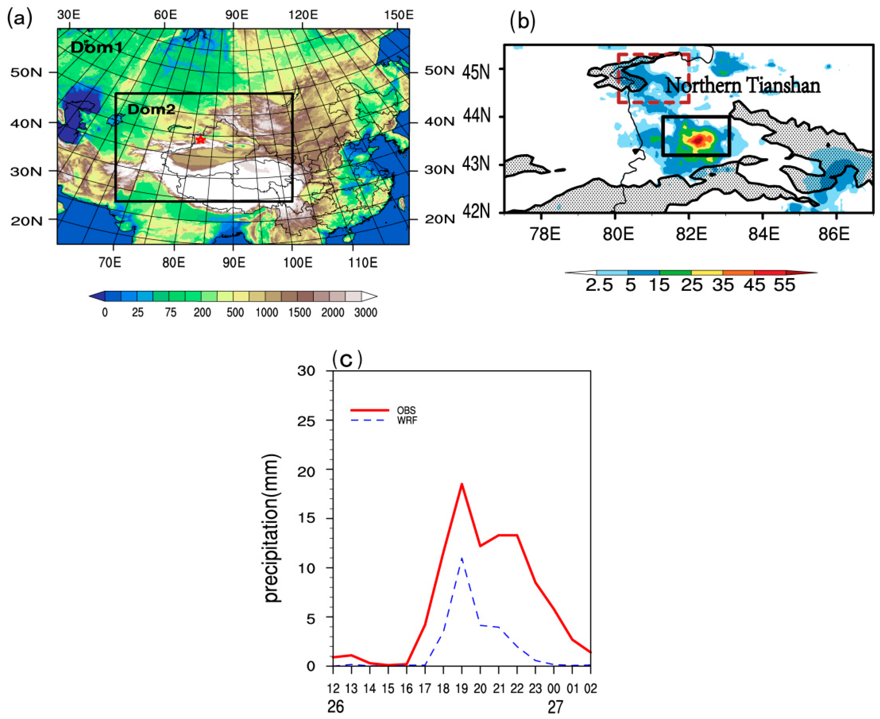
2. Case Overview
3. Model Simulation
3.1. Model Configuration
3.2. Evaluation of the Simulation
4. Mechanisms of the Extreme Precipitation Event
4.1. Spatiotemporal Evolution of Low-Level Systems
4.2. Occurrence and Development of Convection
5. Analysis of the Waves
5.1. Wave Characteristics
5.1.1. Fourier Analysis
5.1.2. Cross-Spectrum Analysis
5.1.3. Wavelet Cross-Spectrum Analysis
5.2. Wave Ducting
5.3. Wave Energy
6. Discussion and Conclusions
- (1)
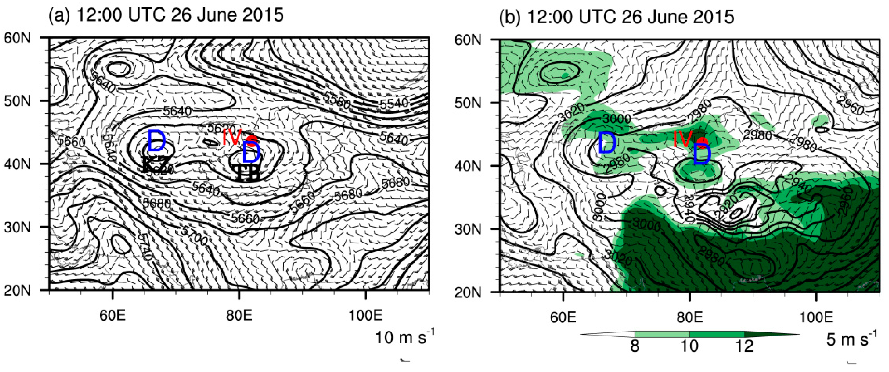
- Our analysis of the circulation based on the observational dataset indicates that there were two stable and slow-moving Central Asian vortices at mid- and lower levels. Affected by both the vortices and the topography, the Ili Valley is mainly controlled by southeasterly winds at 500 hPa; the northerly airflow converges with the westerly winds in the valley at 700 hPa and sufficient water vapor accumulates in the valley at lower levels.
- (2)
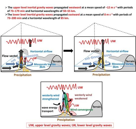
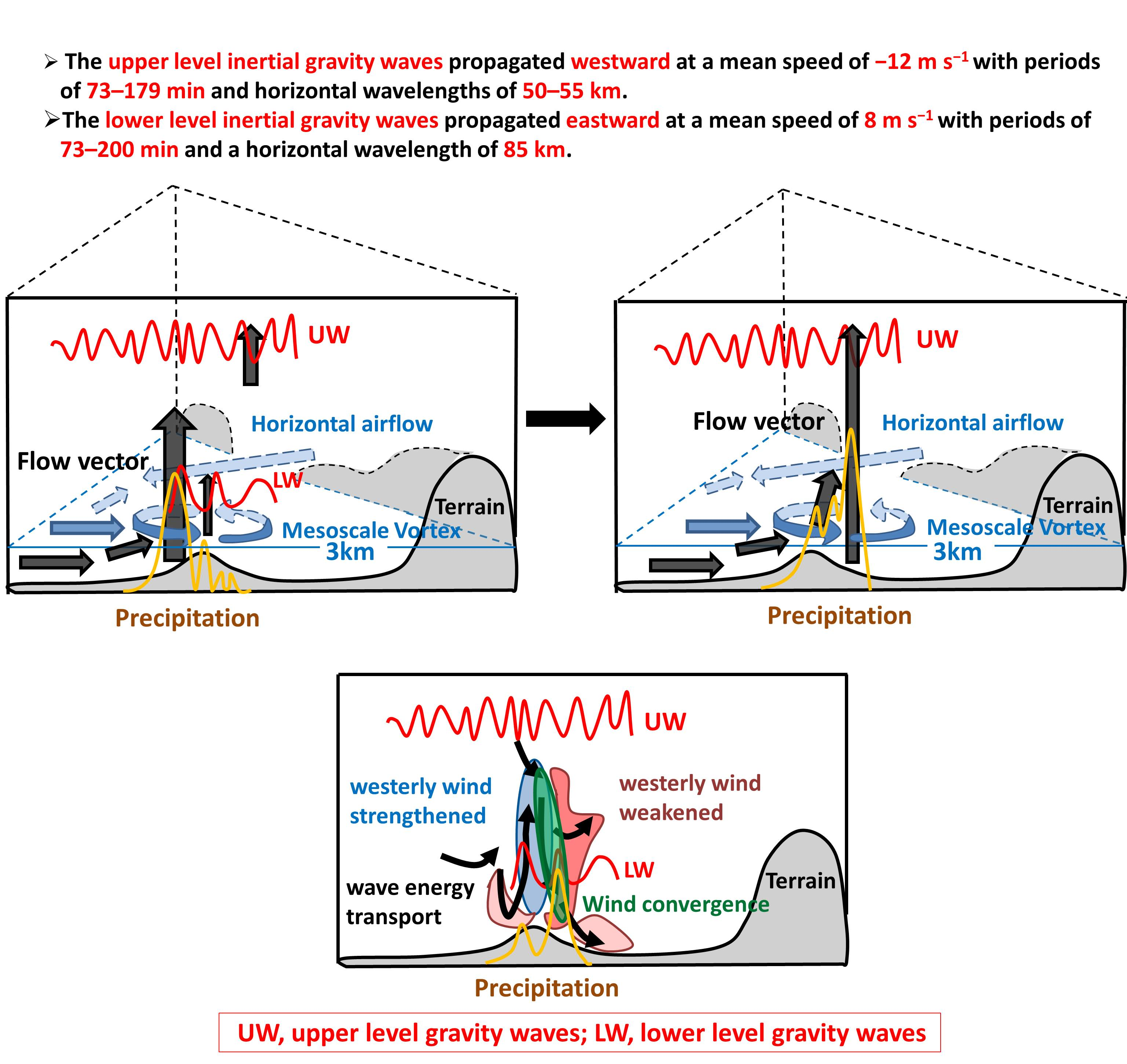
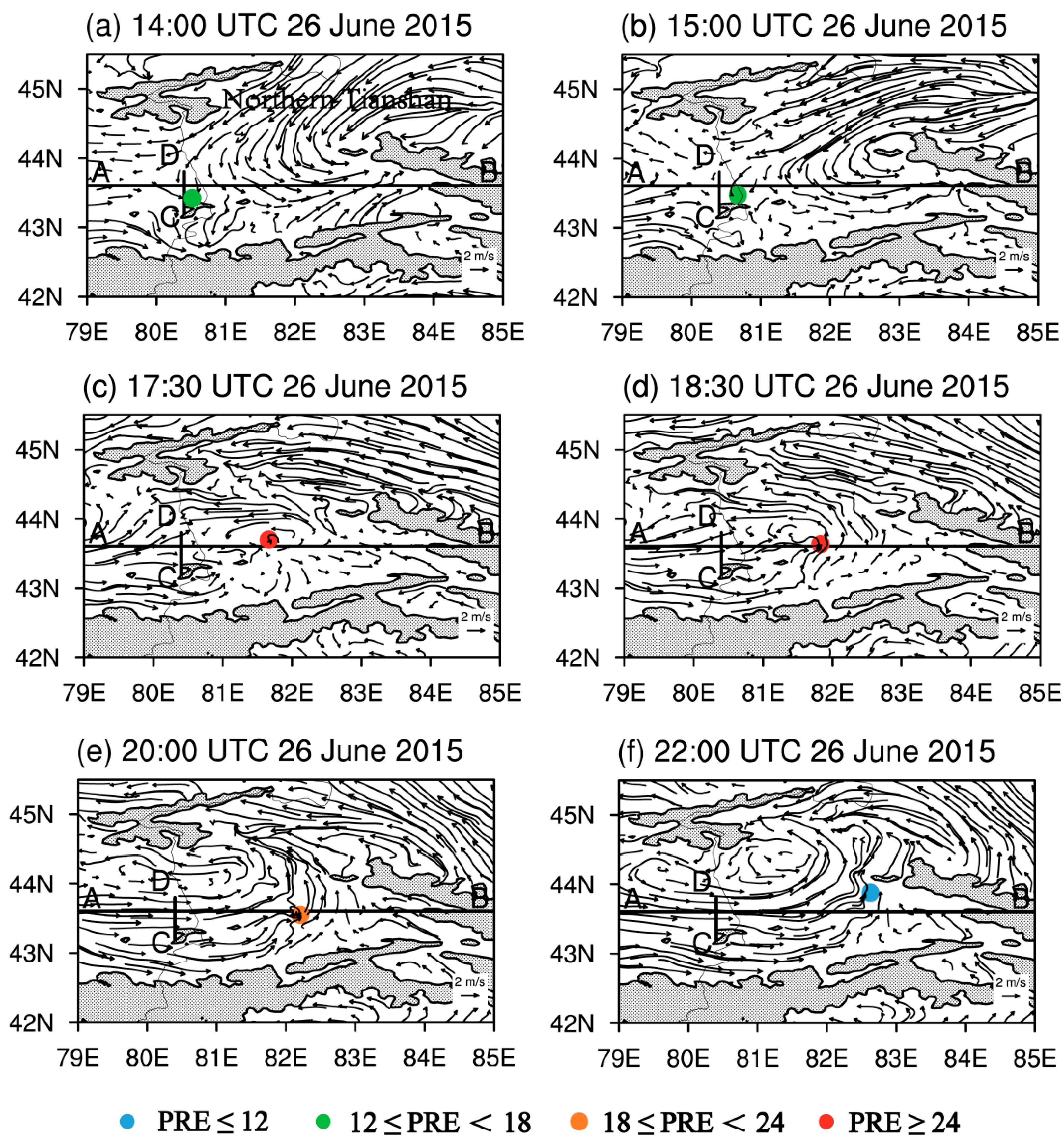
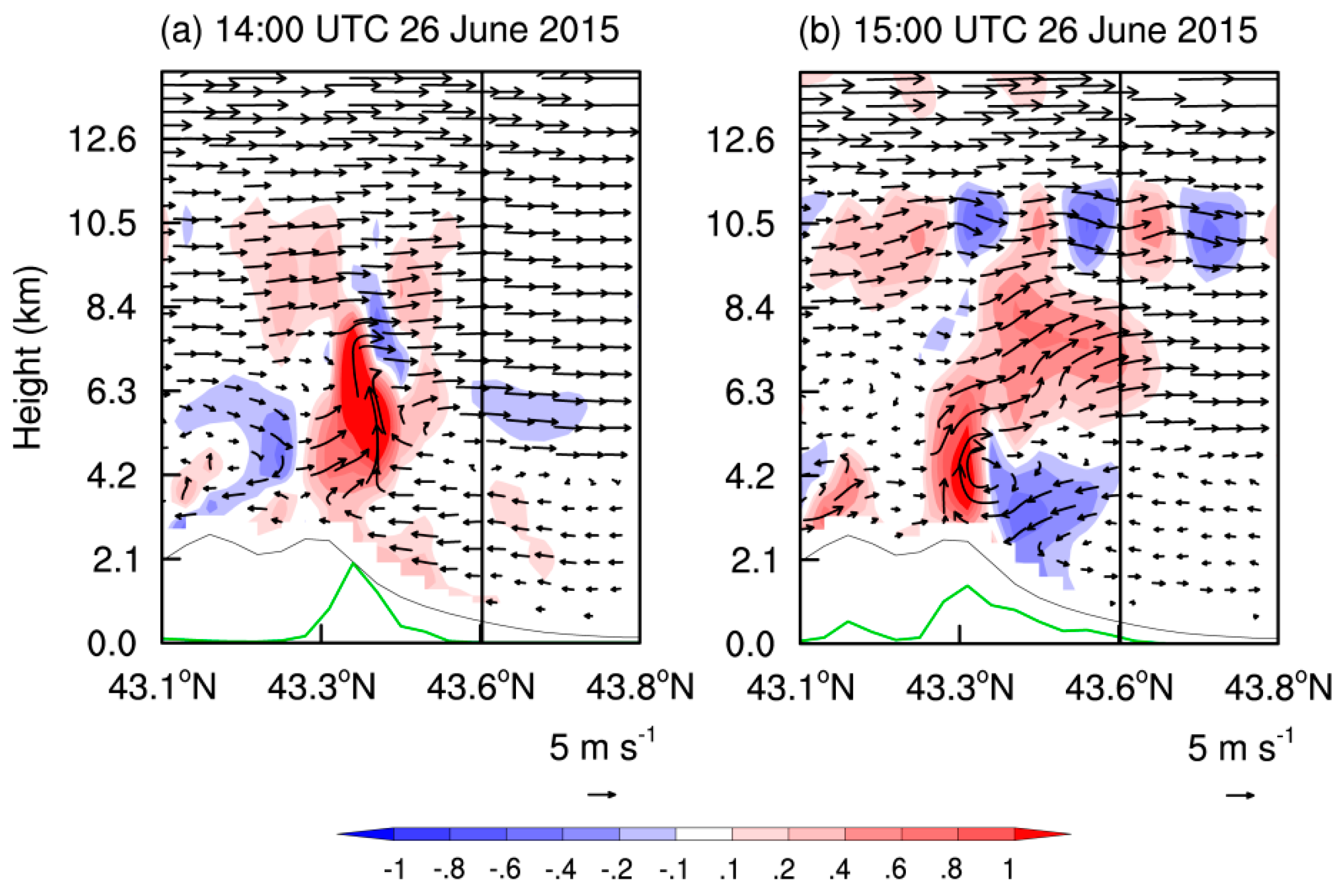
- Based on the WRF simulation, the low-level northerly winds and the westerly winds in the valley formed a mesoscale convergence line in the center of the Ili Valley. A mesoscale vortex formed and developed on the low-level convergence line and the rainfall was distributed near either the convergence line or the mesoscale vortex. The low-level mesoscale convergence line combined with the uplift effect of the upwind slope of the terrain in the center of the Ili Valley to form an ascending motion at lower levels. There was also a relatively strong ascending motion at mid- and high levels as a result of the tilted development of ascending motion caused by terrain uplift and airflow convergence. Convection was triggered and developed rapidly when these two ascending motions were combined and therefore lower level inertial gravity waves were excited. The ascending position of the lower level inertial gravity waves coupled with the convergence of the lower level mesoscale vortex center led to the development of convection and an increase in precipitation. The convection moved eastward to Gongliu County and was vertically coupled with the ascending phase of the upper level inertial gravity waves, which allowed strong convection to develop and the rainfall to significantly intensify.
- (3)
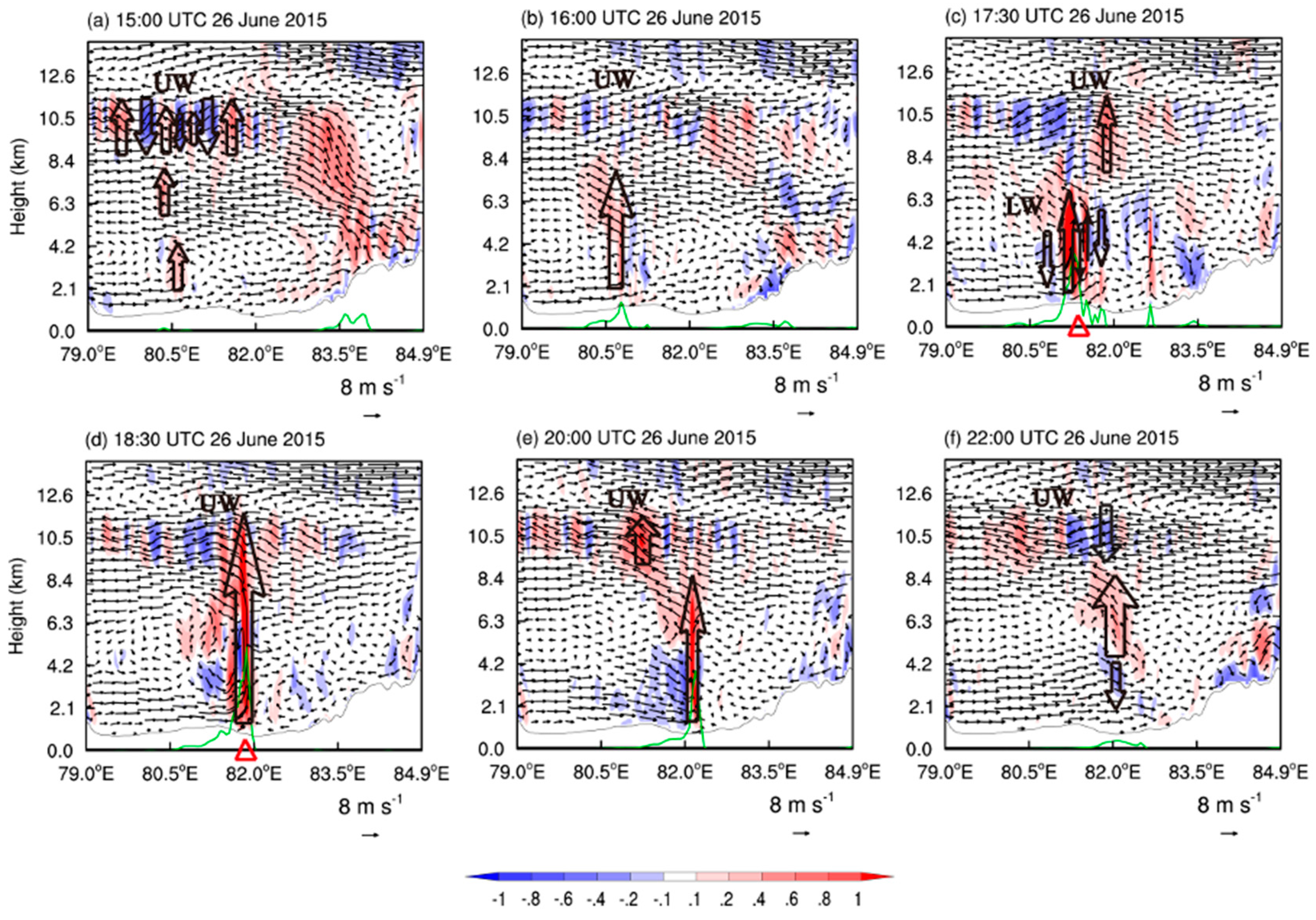
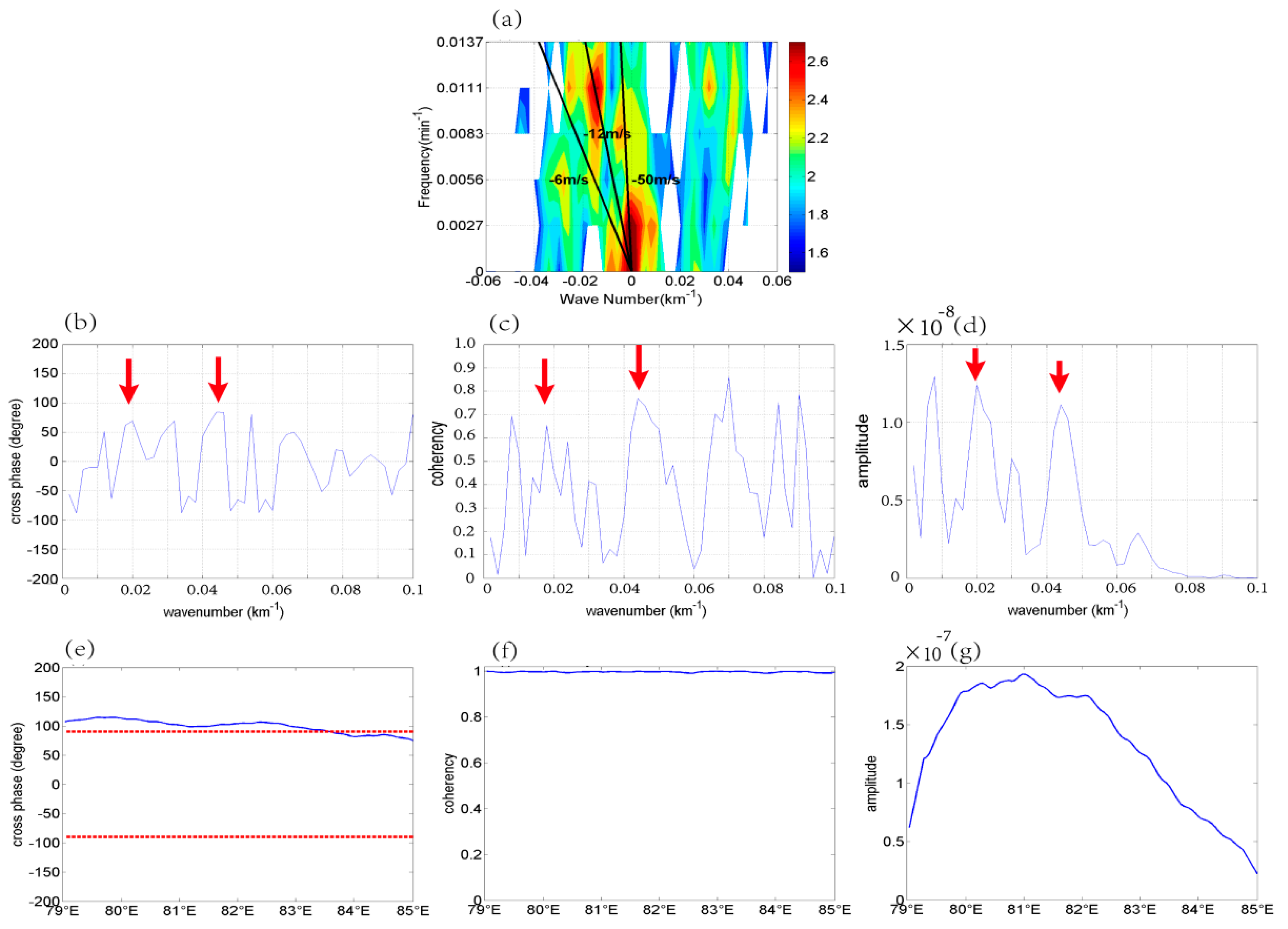
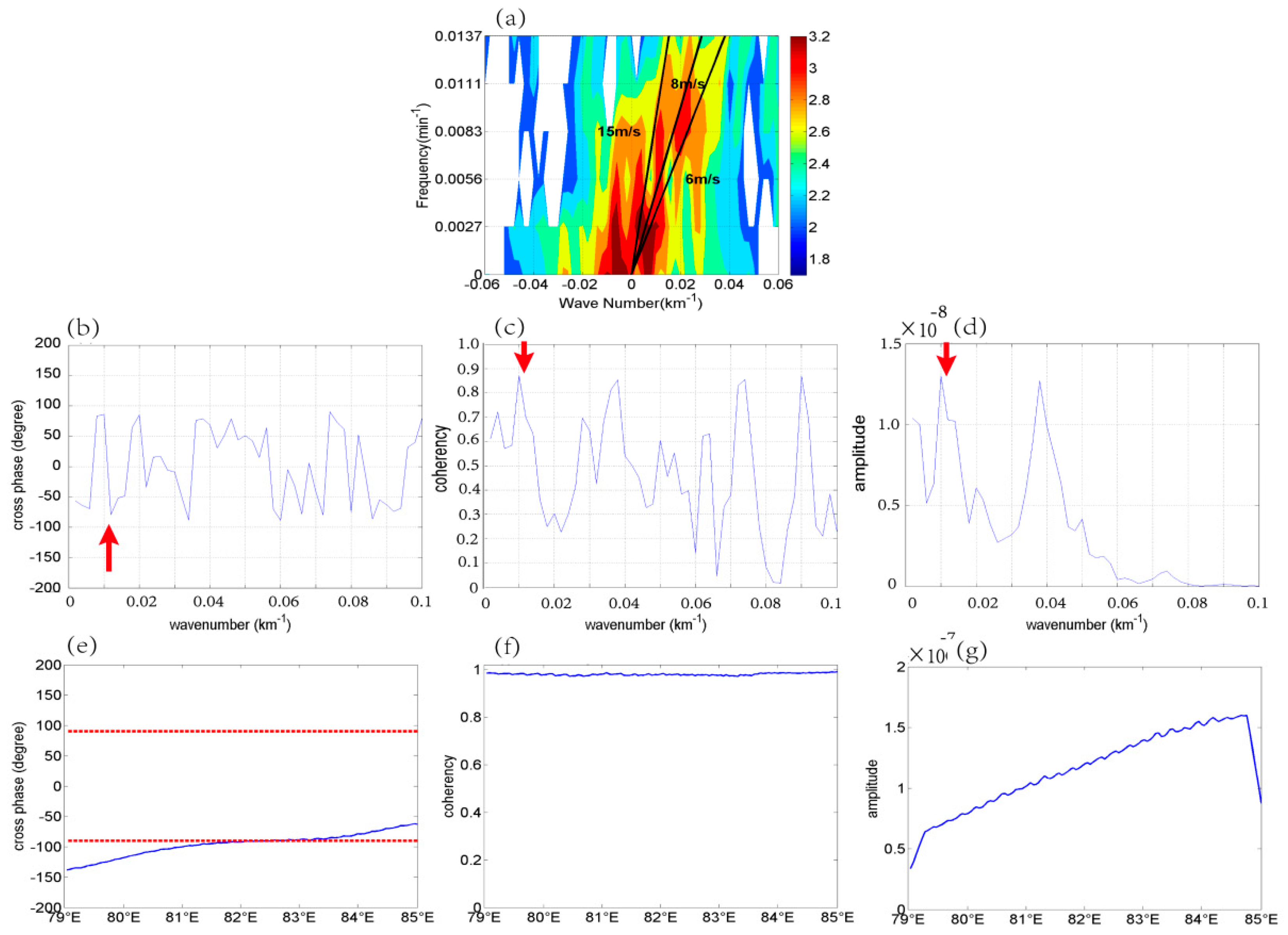
- Spectral analysis methods were used to explore the characteristics of the waves and to identify the wave types. Based on the spectral analysis methods, the upper level waves with horizontal wavelengths of 50–55 km and periods of 73–179 min were mainly located at 79–85° E. The upper level waves propagated westward with a mean wave speed of −12 m s−1 and satisfied the polarization relationship of the westward inertial gravity waves. The upper level inertial gravity waves persisted for a long time and propagated a long distance because of the relatively more favorable waveguide conditions with the critical levels, the strong vertical wind shear and unstable shear energy. The lower level waves with a horizontal wavelength of 85 km and a period of 73–200 min were mainly located at 81–83.5° E. The lower level waves propagated eastward with a mean wave speed of 8 m s−1 and satisfied the polarization relationship of eastward inertial gravity waves. The lower level inertial gravity waves were only maintained for a short time and only propagated over a short distance because of the relatively less favorable waveguide conditions without the critical levels, the strong vertical wind shear and unstable shear energy.
- (4)
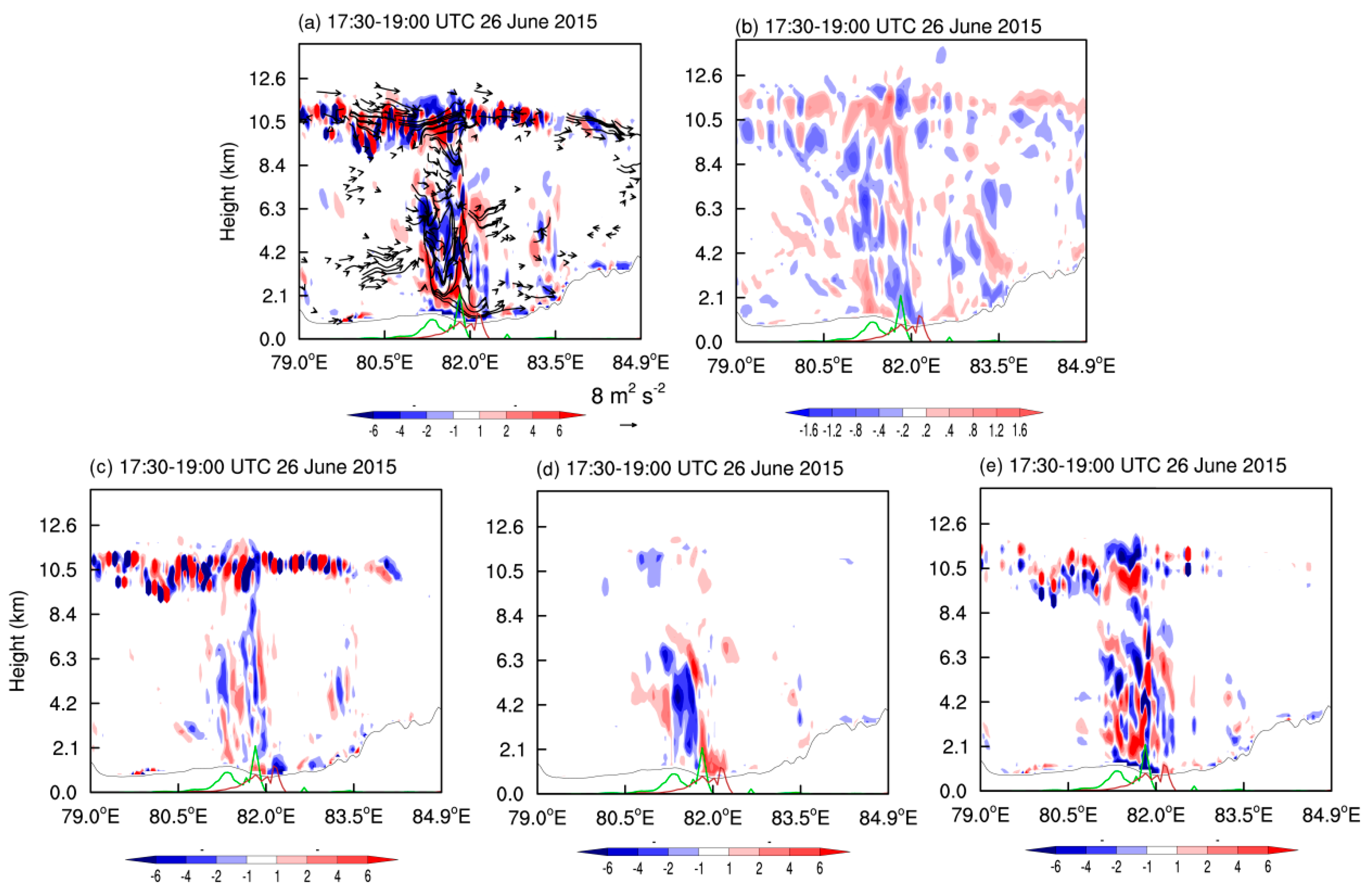
- Based on mesoscale Eliassen–Palm flux theory, the inertial gravity waves can feed back to the mean flow through the transport of wave energy and affect the intensity of the mean wind, enhancing lower and mid-level wind convergence and the mid- and upper level wind divergence. This favors the maintenance and development of convection and precipitation. The mid-level of the convection center was dominated by the meridional transport of zonal momentum, whereas the upper and lower levels of the convection center were dominated by the vertical transport of zonal momentum and the meridional transport of heat.
Author Contributions
Funding
Acknowledgments
Conflicts of Interest
References
- Yang, L.M.; Li, X.; Zhang, G.X. Some advances and problems in the study of heavy rain in Xinjiang. Clim. Environ. Res. 2011, 16, 188–198. (In Chinese) [Google Scholar]
- Zeng, Y.; Zhou, Y.S.; Yang, L.M. A preliminary analysis of the formation mechanism for a heavy rainstorm in western Xinjiang by numerical simulation. Chin. J. Atmos. Sci. 2019, 43, 372–388. (In Chinese) [Google Scholar]
- Zhang, J.B.; Deng, Z.F. Introduction to Precipitation in Xinjiang; Meteorological Press: Beijing, China, 1987. (In Chinese) [Google Scholar]
- Liao, F.; Hong, Y.C.; Zheng, G.G. Review of orographic influences on surface precipitation. Meteorol. Sci. Technol. 2007, 35, 309–316. (In Chinese) [Google Scholar]
- Smith, R. The influence of mountains on the atmosphere. Adv. Geophys. 1979, 21, 87–230. [Google Scholar]
- Houze, R.A., Jr. Orographic effects on precipitating clouds. Rev. Geophys. 2012, 50. [Google Scholar] [CrossRef]
- Roe, G.H. Orographic precipitation. Annu. Rev. Earth Planet. Sci. 2005, 33, 645–671. [Google Scholar] [CrossRef]
- Rudari, R.; Entekhabi, D.; Roth, G. Terrain and multiple-scale interactions as factors in generating extreme precipitation events. J. Hydrometeorol. 2004, 5, 390–404. [Google Scholar] [CrossRef]
- Tao, S.Y. Rainstorms in China; Science Press: Beijing, China, 1980. (In Chinese) [Google Scholar]
- Gao, K.; Zhai, G.Q.; Yu, Z.X.; Tu, C.H. The simulation study of the meso-scale orographic effects on heavy rain in East China. Sci. Atmos. Sin. 1994, 52, 157–164. (In Chinese) [Google Scholar]
- Li, B.; Liu, L.P.; Zhao, S.X.; Huang, C.Y. Numerical experiment of the effect of local low terrain on heavy rainstorm of South China. Plateau Meteorol. 2013, 32, 1638–1650. (In Chinese) [Google Scholar]
- Pierrehumbert, R.T. Linear results on the barrier effects of mesoscale mountains. J. Atmos. Sci. 1984, 41, 1356–1367. [Google Scholar] [CrossRef][Green Version]
- Pierrehumbert, R.T.; Wyman, B. Upstream effects of mesoscale mountains. J. Atmos. Sci. 1985, 42, 977–1003. [Google Scholar] [CrossRef]
- Sun, J.S. The effects of vertical distribution of the lower level flow on precipitation location. Plateau Meteorol. 2005, 24, 62–69. (In Chinese) [Google Scholar]
- Zang, Z.L.; Zhang, M.; Shen, H.W.; Yao, H.H. Experiments on the sentivity of meso-scale terrains in Janghuai area to a heavy mold rain. Sci. Meteorol. Sin. 2004, 24, 26–34. (In Chinese) [Google Scholar]
- Zhu, M.; Yu, Z.H.; Lu, H.C. The effect of meso-scale lee wave and its application. Acta Meteorol. Sin. 1999, 57, 705–714. (In Chinese) [Google Scholar]
- Wang, J.; Shen, X.Y.; Shou, S.W.; Xu, Z.F. Numerical simulation and analysis of influence of complex topography on a Fujian rainstorm. J. Nanjing Inst. Meteorol. 2008, 30, 546–554. (In Chinese) [Google Scholar]
- Li, Z.G.; Liang, B.Q.; Bao, C.L. The Causes and Forecasting Problems of Heavy Rain of Early-Summer Rainstorms in Southern China; Meteorological Press: Beijing, China, 1981. (In Chinese) [Google Scholar]
- Sun, M.S.; Yang, L.Q.; Yin, Q.; Niu, Z.Y.; Gao, L.M. Analysis on the cause of a torrential rain occurring in Beijing on 21 July 2012(II):Vertical motion, wind vertical shear and terrain effect. Torrential Rain Disasters 2013, 32, 218–223. [Google Scholar]
- Huang, X.; Zhou, Y.S.; Ran, L.K.; Kalim, U.; Zeng, Y. Analysis of environment field and unstable condition on a rainstorm event in Ili Valley of Xinjiang. Chin. J. Atmos. Sci. 2020. in Press. [Google Scholar] [CrossRef]
- Zheng, B.H.; Li, B.; Huang, Q.X.; Li, R.Q.; Zhao, K.M. Diurnal variation characteristics of precipitation in the cold and warm season of Ili River Valley, Xinjiang. Desert Oasis Meteorol. 2019, 13, 80–87. (In Chinese) [Google Scholar]
- Bretherton, C.S.; Smolarkiewicz, P.K. Gravity-waves, compensating subsidence and detrainment around cumulus clouds. J. Atmos. Sci. 1989, 46, 740–759. [Google Scholar] [CrossRef]
- Fovell, R.G.; Mullendore, G.L.; Kim, S.-H. Discrete propagation in numerically simulated nocturnal squall lines. Mon. Weather Rev. 2006, 134, 3735–3752. [Google Scholar] [CrossRef]
- Li, M.C. The triggering effect of gravity wave on heavy rain. Sci. Atmos. Sin. 1978, 02, 201–209. (In Chinese) [Google Scholar]
- Liu, J.; Wang, W. Characteristics of gravity wave during a rainstorm process. J. Arid Meteorol. 2010, 28, 65–70+75. (In Chinese) [Google Scholar]
- Ma, Z.F. The relations between the index of low-frequency gravitational wave and heavy rain proceed from developmentof southwest vortex. Plateau Meteorol. 1994, 13, 51–57. (In Chinese) [Google Scholar]
- Nicholls, M.E.; Pielke, R.A.; Cotton, W.R. Thermally forced gravity-waves in an atmosphere at rest. J. Atmos. Sci. 1991, 48, 1869–1884. [Google Scholar] [CrossRef]
- Sharman, R.D.; Wurtele, M.G. Three-dimensional structure of forced gravity waves and lee waves. J. Atmos. Sci. 2004, 61, 664–681. [Google Scholar] [CrossRef]
- Stobie, J.G.; Einaudi, F.; Uccellini, L.W. A case-study of gravity-waves convective storms interaction—9 May 1979. J. Atmos. Sci. 1983, 40, 2804–2830. [Google Scholar] [CrossRef]
- Su, T.; Zhai, G. The role of convectively generated gravity waves on convective initiation: A case study. Mon. Weather Rev. 2017, 145, 335–359. [Google Scholar] [CrossRef]
- Uccellini, L.W.; Koch, S.E. The synoptic setting and possible energy-sources for mesoscale wave disturbances. Mon. Weather Rev. 1987, 115, 721–729. [Google Scholar] [CrossRef]
- Wang, W.; Liu, J.; Cai, X.J. Impact of mesoscale gravity waves on a heavy rainfall event in the east side of the Tibetan Plateau. Trans. Atmos. Sci. 2011, 34, 737–747. (In Chinese) [Google Scholar]
- Xu, X.F.; Sun, Z.B. Dynamic studyon influence of gravity wave induced by unbalanced flow on Meiyu front heavy rain. Acta Meteorol. Sin. 2003, 61, 655–660+790-793. (In Chinese) [Google Scholar]
- Zhang, F.Q.; Koch, S.E.; Davis, C.A.; Kaplan, M.L. Wavelet analysis and the governing dynamics of a large-amplitude mesoscale gravity-wave event along the East Coast of the United States. Q. J. R. Meteorol. Soc. 2001, 127, 2209–2245. [Google Scholar] [CrossRef]
- Yang, R.; Liu, Y.; Ran, L.K.; Zhang, Y.L. Simulation of a torrential rainstorm in Xinjiang and gravity wave analysis. Chin. Phys. B 2018, 27, 059201. [Google Scholar] [CrossRef]
- Fovell, R.; Durran, D.; Holton, J.R. Numerical simulations of convectively generated stratospheric gravity-waves. J. Atmos. Sci. 1992, 49, 1427–1442. [Google Scholar] [CrossRef]
- Piani, C.; Durran, D.; Alexander, M.J.; Holton, J.R. A numerical study of three-dimensional gravity waves triggered by deep tropical convection and their role in the dynamics of the QBO. J. Atmos. Sci. 2000, 57, 3689–3702. [Google Scholar] [CrossRef]
- Liu, L.; Ran, L.; Gao, S. Analysis of the characteristics of inertia-gravity waves during an orographic precipitation event. Adv. Atmos. Sci. 2018, 35, 604–620. [Google Scholar] [CrossRef]
- Du, Y.; Zhang, F. Banded convective activity associated with mesoscale gravity waves over southern China. J. Geophys. Res. -Atmos. 2019, 124, 1912–1930. [Google Scholar] [CrossRef]
- Lane, T.P.; Zhang, F. Coupling between gravity waves and tropical convection at mesoscales. J. Atmos. Sci. 2011, 68, 2582–2598. [Google Scholar] [CrossRef]
- Wheeler, M.; Kiladis, G.N. Convectively coupled equatorial waves: Analysis of clouds and temperature in the wavenumber-frequency domain. J. Atmos. Sci. 1999, 56, 374–399. [Google Scholar] [CrossRef]
- Chen, C.; Chu, X.; McDonald, A.J.; Vadas, S.L.; Yu, Z.; Fong, W.; Lu, X. Inertia-gravity waves in Antarctica: A case study using simultaneous lidar and radar measurements at McMurdo/Scott Base (77.8 degrees S, 166.7 degrees E). J. Geophys. Res. Atmos. 2013, 118, 2794–2808. [Google Scholar] [CrossRef]
- Chen, D.; Chen, Z.Y.; LÜ, D.R. Spatiotemporal spectrum and momentum flux of the stratospheric gravity waves generated by a typhoon. Sci. China: Earth Sci. 2013, 43, 889–897. (In Chinese) [Google Scholar] [CrossRef]
- Lane, T.P.; Moncrieff, M.W. Stratospheric gravity waves generated by multiscale tropical convection. J. Atmos. Sci. 2008, 65, 2598–2614. [Google Scholar] [CrossRef]
- Zhang, Y.C.; Zhang, F.Q.; Sun, J.H. Comparison of the diurnal variations of warm-season precipitation for East Asia vs. North America downstream of the Tibetan Plateau vs. the Rocky Mountains. Atmos. Chem. Phys. 2014, 14, 10741–10759. [Google Scholar] [CrossRef]
- Cai, X.; Yuan, T.; Zhao, Y.; Pautet, P.-D.; Taylor, M.J.; Pendleton, W.R., Jr. A coordinated investigation of the gravity wave breaking and the associated dynamical instability by a Na lidar and an Advanced Mesosphere Temperature Mapper over Logan, UT (41.7 degrees N, 111.8 degrees W). J. Geophys. Res. Space Phys. 2014, 119, 6852–6864. [Google Scholar] [CrossRef]
- Gao, S.T.; Ran, L.K.; Li, X.F. The Mesoscale Dynamic Meteorology and Its Prediction Method; Meteorological Press: Beijing, China, 2015. (In Chinese) [Google Scholar]
- Lu, C.G.; Koch, S.; Wang, N. Determination of temporal and spatial characteristics of atmospheric gravity waves combining cross-spectral analysis and wavelet transformation. J. Geophys. Res. Atmos. 2005, 110. [Google Scholar] [CrossRef]
- Lu, C.U.; Koch, S.E.; Wang, N. Stokes parameter analysis of a packet of turbulence-generating gravity waves. J. Geophys. Res. Atmos. 2005, 110. [Google Scholar] [CrossRef]
- Gamage, N.; Blumen, W. Comparative-analysis of low-level cold fronts—Wavelet, fourier, and empirical orthogonal function decompositions. Mon. Weather Rev. 1993, 121, 2867–2878. [Google Scholar] [CrossRef]
- Grivet-Talocia, S.; Einaudi, F.; Clark, W.L.; Dennett, R.D.; Nastrom, G.D.; VanZandt, T.E. A 4-yr climatology of pressure disturbances using a barometer network in central Illinois. Mon. Weather Rev. 1999, 127, 1613–1629. [Google Scholar] [CrossRef][Green Version]
- Lu, X.; Chen, C.; Huang, W.; Smith, J.A.; Chu, X.; Yuan, T.; Pautet, P.-D.; Taylor, M.J.; Gong, J.; Cullens, C.Y. A coordinated study of 1 h mesoscale gravity waves propagating from Logan to Boulder with CRRL Na Doppler lidars and temperature mapper. J. Geophys. Res. Atmos. 2015, 120, 10006–10021. [Google Scholar] [CrossRef]
- Weng, H.Y.; Lau, K.M. Wavelets, period-doubling, and time-frequency localization with application to organization of convection over the tropical Western Pacific. J. Atmos. Sci. 1994, 51, 2523–2541. [Google Scholar] [CrossRef]
- Yuan, T.; Heale, C.J.; Snively, J.B.; Cai, X.; Pautet, P.D.; Fish, C.; Zhao, Y.; Taylor, M.J.; Pendleton, W.R., Jr.; Wickwar, V.; et al. Evidence of dispersion and refraction of a spectrally broad gravity wave packet in the mesopause region observed by the Na lidar and Mesospheric Temperature Mapper above Logan, Utah. J. Geophys. Res. -Atmos. 2016, 121, 579–594. [Google Scholar] [CrossRef]
- Lee, D. Analysis of phase-locked oscillations in multi-channel single-unit spike activity with wavelet cross-spectrum. J. Neurosci. Methods 2002, 115, 67–75. [Google Scholar] [CrossRef]
- Torrence, C.; Compo, G.P. A practical guide to wavelet analysis. Bull. Am. Meteorol. Soc. 1998, 79, 61–78. [Google Scholar] [CrossRef]
- Lomb, N.R. Least-squares frequency-analysis of unequally spaced data. Astrophys. Space Sci. 1976, 39, 447–462. [Google Scholar] [CrossRef]
- Scargle, J.D. Studies in astronomical time-series analysis. 2. Statistical aspects of spectral-analysis of unevenly spaced data. Astrophys. J. 1982, 263, 835–853. [Google Scholar] [CrossRef]
- VanderPlas, J.T. Understanding the Lomb-Scargle Periodogram. Astrophys. J. Suppl. Ser. 2018, 236, 16. [Google Scholar] [CrossRef]
- Cai, X.; Yuan, T.; Liu, H.-L. Large-scale gravity wave perturbations in the mesopause region above Northern Hemisphere midlatitudes during autumnal equinox: A joint study by the USU Na lidar and Whole Atmosphere Community Climate Model. Ann. Geophys. 2017, 35, 181–188. [Google Scholar] [CrossRef]
- Ford, E.A.K.; Aruliah, A.L.; Griffin, E.M.; McWhirter, I. Statistical analysis of thermospheric gravity waves from Fabry-Perot Interferometer measurements of atomic oxygen. Ann. Geophys. 2008, 26, 29–45. [Google Scholar] [CrossRef]
- Eliassen, A.; Palm, E. On the transfer of energy in stationary mountain waves. Geofys. Publ. 1961, 22, 1–23. [Google Scholar]
- Andrews, D.G.; McIntyre, M.E. Planetary waves in horizontal and vertical shear—Generalized Eliassen-Palm relation and mean zonal acceleration. J. Atmos. Sci. 1976, 33, 2031–2048. [Google Scholar] [CrossRef]
- Andrews, D.G.; McIntyre, M.E. Generalized Eliassen-Palm and Charney-Drazin theorems for waves on axisymmetric mean flows in compressible atmospheres. J. Atmos. Sci. 1978, 35, 175–185. [Google Scholar]
- Gao, S.T.; Tao, S.Y.; Ding, Y.H. The generalized E-P flux that characterizes the interaction between wave and flow. Sci. China (Ser. B) 1989, 774–784. (In Chinese) [Google Scholar] [CrossRef]
- Hoskins, B.J.; James, I.N.; White, G.H. The shape, propagation and mean-flow interaction of large-scale weather systems. J. Atmos. Sci. 1983, 40, 1595–1612. [Google Scholar] [CrossRef]
- Huang, R.H. The role of Greenland Plateau in the formation of the northern hemispheric stationary planetary waves in winter. Sci. Atmos. Sin. 1983, 07, 393–402. (In Chinese) [Google Scholar]
- Huang, R.H.; Kanzaburo, G. A study on the steady propagation of the planetary wave in the northern hemisphere in another waveguide in winter. Sci. China (Ser. B) 1983, 10, 940–950. (In Chinese) [Google Scholar]
- Kinoshita, T.; Sato, K. A formulation of three-dimensional residual mean flow applicable both to inertia-gravity waves and to Rossby waves. J. Atmos. Sci. 2013, 70, 1577–1602. [Google Scholar] [CrossRef]
- Kinoshita, T.; Sato, K. A formulation of unified three-dimensional wave activity flux of inertia-gravity waves and Rossby waves. J. Atmos. Sci. 2013, 70, 1603–1615. [Google Scholar] [CrossRef]
- Kinoshita, T.; Tomikawa, Y.; Sato, K. On the three-dimensional residual mean circulation and wave activity flux of the primitive equations. J. Meteorol. Soc. Jpn. 2010, 88, 373–394. [Google Scholar] [CrossRef]
- Miyahara, S. A three dimensional wave activity flux applicable to inertio-gravity waves. Sola 2006, 2, 108–111. [Google Scholar] [CrossRef][Green Version]
- Plumb, R.A. On the 3-dimensional propagation of stationary waves. J. Atmos. Sci. 1985, 42, 217–229. [Google Scholar] [CrossRef]
- Plumb, R.A. 3-dimensional propagation of transient quasi-geostrophic eddies and its relationship with the eddy forcing of the time mean flow. J. Atmos. Sci. 1986, 43, 1657–1678. [Google Scholar] [CrossRef]
- Scinocca, J.F.; Shepherd, T.G. Nonlinear wave-activity conservation-laws and Hamiltonian-structure for the 2-dimensional anelastic equations. J. Atmos. Sci. 1992, 49, 5–27. [Google Scholar] [CrossRef]
- Takaya, K.; Nakamura, H. A formulation of a wave-activity flux for stationary Rossby waves on a zonally varying basic flow. Geophys. Res. Lett. 1997, 24, 2985–2988. [Google Scholar] [CrossRef]
- Takaya, K.; Nakamura, H. A formulation of a phase-independent wave-activity flux for stationary and migratory quasigeostrophic eddies on a zonally varying basic flow. J. Atmos. Sci. 2001, 58, 608–627. [Google Scholar] [CrossRef]
- Tung, K.K. Nongeostrophic theory of zonally averaged circulation. 1. Formulation. J. Atmos. Sci. 1986, 43, 2600–2618. [Google Scholar] [CrossRef][Green Version]
- Wu, G.X.; Chen, B. Non-acceleration theorem in a primitive Equation system: I. Acceleration of zonal meanflow. Adv. Atmos. Sci. 1989, 6, 1–20. [Google Scholar]
- Xu, X.D.; Gao, S.T. The Theorem of External Forcing and Wave-Flow Interaction; Ocean Press: Beijing, China, 2002. (In Chinese) [Google Scholar]
- Chen, W.; Huang, R.H. A Numerical Study of Seasonal and Interannual Variabilities of Ozone due to Planetary Wave Transport in the Middle Atmosphere Part II. The Case of Wave- Flow Interaction. Sci. Atmos. Sin. 1996, 20, 64–73. (In Chinese) [Google Scholar]
- Gao, S.T.; Tao, S.Y. The lower layer frontogenesis induced by the acceleration of upper jet stream. Sci. Atmospheirca Sin. 1991, 15, 11–22. (In Chinese) [Google Scholar]
- Ran, L.K.; Gao, S.T.; Lei, T. Relation between acceleration of basic zonal flow and EP flux in the upper-level jet stream region. Chin. J. Atmos. Sci. 2005, 29, 409–416. (In Chinese) [Google Scholar]
- Liu, L.; Ran, L.; Gao, S. A three-dimensionalwave activity flux of inertia-gravity waves and its application to a rainstorm event. Adv. Atmos. Sci. 2019, 36, 206–218. [Google Scholar] [CrossRef]
- Shen, Y.; Pan, Y.; Yu, J.; Zhao, P.; Zhou, Z. Quality assessment of hourly merged precipitation product over China. Trans. Atmos. Sci. 2013, 36, 37–46. (In Chinese) [Google Scholar]
- Dee, D.P.; Uppala, S.M.; Simmons, A.J.; Berrisford, P.; Poli, P.; Kobayashi, S.; Andrae, U.; Balmaseda, M.A.; Balsamo, G.; Bauer, P.; et al. The ERA-Interim reanalysis: Configuration and performance of the data assimilation system. Q. J. R. Meteorol. Soc. 2011, 137, 553–597. [Google Scholar] [CrossRef]
- Huang, Y.; Liu, T.; Zhang, Y.H. Features of a Regional Rainstorm in Midsummer of 2010 in Western Xinjiang. J. Arid Meteorol. 2012, 30, 615–622. (In Chinese) [Google Scholar]
- Zhang, Y.H.; Chen, C.Y.; Yang, L.M.; Jia, L.H.; Yang, X. Cause analysis on rare rainstorm in west of southern Xinjiang. Plateau Meteorol. 2013, 32, 191–200. (In Chinese) [Google Scholar]
- Morrison, H.; Thompson, G.; Tatarskii, V. Impact of cloud microphysics on the development of trailing stratiform precipitation in a simulated squall line: Comparison of one- and two-moment schemes. Mon. Weather Rev. 2009, 137, 991–1007. [Google Scholar] [CrossRef]
- Pleim, J.E. A combined local and nonlocal closure model for the atmospheric boundary layer. Part I: Model description and testing. J. Appl. Meteorol. Climatol. 2007, 46, 1383–1395. [Google Scholar] [CrossRef]
- Kain, J.S. The Kain-Fritsch convective parameterization: An update. J. Appl. Meteorol. 2004, 43, 170–181. [Google Scholar] [CrossRef]
- Clark, T.L.; Hauf, T.; Kuettner, J.P. Convectively forced internal gravity-waves—Results from two-dimensional numerical experiments. Q. J. R. Meteorol. Soc. 1986, 112, 899–925. [Google Scholar] [CrossRef]
- Ding, X. Gravity Waves Generated by Convection and Their Interactions with Mean Flow; Wuhan University: Wuhan, China, 2011. (In Chinese) [Google Scholar]
- McLandress, C.; Alexander, M.J.; Wu, D.L. Microwave Limb Sounder observations of gravity waves in the stratosphere: A climatology and interpretation. J. Geophys. Res. Atmos. 2000, 105, 11947–11967. [Google Scholar] [CrossRef]
- Misiti, M.Y.; Misiti, G. Oppenheim. Wavelet Toolbox; The MathWorks Inc.: Natick, MA, USA, 1996. [Google Scholar]
- Lindzen, R.S.; Tung, K.K. Banded convective activity and ducted gravity-waves. Mon. Weather Rev. 1976, 104, 1602–1617. [Google Scholar] [CrossRef]
- Andrioli, V.F.; Batista, P.P.; Xu, J.; Yang, G.; Wang, C.; Liu, Z. Strong temperature gradients and vertical wind shear on MLT region associated to instability source at 23 degrees S. J. Geophys. Res. Space Phys. 2017, 122, 4500–4511. [Google Scholar] [CrossRef]
- Yuan, T.; Pautet, P.D.; Zhao, Y.; Cai, X.; Criddle, N.R.; Taylor, M.J.; Pendleton, W.R., Jr. Coordinated investigation of midlatitude upper mesospheric temperature inversion layers and the associated gravity wave forcing by Na lidar and Advanced Mesospheric Temperature Mapper in Logan, Utah. J. Geophys. Res. Atmos. 2014, 119, 3756–3769. [Google Scholar] [CrossRef]
- Zhang, F.Q.; Koch, S.E.; Kaplan, M.L. Numerical simulations of a large-amplitude mesoscale gravity wave event. Meteorol. Atmos. Phys. 2003, 84, 199–216. [Google Scholar] [CrossRef]
- Lund, T.S.; Wu, X.H.; Squires, K.D. Generation of turbulent inflow data for spatially-developing boundary layer simulations. J. Comput. Phys. 1998, 140, 233–258. (In English) [Google Scholar] [CrossRef]
- Spalart, P.R.; Deck, S.; Shur, M.L.; Squires, K.D.; Strelets, M.K.; Travin, A. A new version of detached-eddy simulation, resistant to ambiguous grid densities. Theor. Comput. Fluid Dyn. 2006, 20, 181–195. (In English) [Google Scholar] [CrossRef]
- Caccamo, M.T.; Castorina, G.; Colombo, F.; Insinga, V.; Maiorana, E.; Magazu, S. Weather forecast performances for complex orographic areas: Impact of different grid resolutions and of geographic data on heavy rainfall event simulations in Sicily. Atmos. Res. 2017, 198, 22–33. (In English) [Google Scholar] [CrossRef]
- Castorina; Caccamo, M.T.; Magazù, S. Study of convective motions and analysis of the impact of physical parametrization on the WRF-ARW forecast model. AAPP Atti della Accademia Peloritana dei Pericolanti, Classe di Scienze Fisiche, Matematiche e Naturali 2019, 97, A20. [Google Scholar]


© 2020 by the authors. Licensee MDPI, Basel, Switzerland. This article is an open access article distributed under the terms and conditions of the Creative Commons Attribution (CC BY) license (http://creativecommons.org/licenses/by/4.0/).
Share and Cite
Huang, X.; Zhou, Y.; Liu, L. Occurrence and Development of an Extreme Precipitation Event in the Ili Valley, Xinjiang, China and Analysis of Gravity Waves. Atmosphere 2020, 11, 752. https://doi.org/10.3390/atmos11070752
Huang X, Zhou Y, Liu L. Occurrence and Development of an Extreme Precipitation Event in the Ili Valley, Xinjiang, China and Analysis of Gravity Waves. Atmosphere. 2020; 11(7):752. https://doi.org/10.3390/atmos11070752
Chicago/Turabian StyleHuang, Xin, Yushu Zhou, and Lu Liu. 2020. "Occurrence and Development of an Extreme Precipitation Event in the Ili Valley, Xinjiang, China and Analysis of Gravity Waves" Atmosphere 11, no. 7: 752. https://doi.org/10.3390/atmos11070752
APA StyleHuang, X., Zhou, Y., & Liu, L. (2020). Occurrence and Development of an Extreme Precipitation Event in the Ili Valley, Xinjiang, China and Analysis of Gravity Waves. Atmosphere, 11(7), 752. https://doi.org/10.3390/atmos11070752