Article

Evaluation of Rainfall Forecasts by Three Mesoscale Models during the Mei-Yu Season of 2008 in Taiwan. Part III: Application of an Object-Oriented Verification Method

1
Department of Earth Sciences, National Taiwan Normal University, Taipei 106, Taiwan
2
Department of Environmental Atmospheric Sciences, Pukyong National University, Busan 48513, Korea
*
Author to whom correspondence should be addressed.
Atmosphere 2020, 11(7), 705; https://doi.org/10.3390/atmos11070705
Submission received: 5 June 2020 / Revised: 30 June 2020 / Accepted: 30 June 2020 / Published: 2 July 2020
(This article belongs to the Section Meteorology)

Abstract

:
In this study, the performances of Mei-yu (May–June) quantitative precipitation forecasts (QPFs) in Taiwan by three mesoscale models: the Cloud-Resolving Storm Simulator (CReSS), the Central Weather Bureau (CWB) Weather Research and Forecasting (WRF), and the CWB Non-hydrostatic Forecast System (NFS) are explored and compared using an newly-developed object-oriented verification method, with particular focus on the various properties or attributes of rainfall objects identified. Against a merged dataset from ~400 rain gauges in Taiwan and the Tropical Rainfall Measuring Mission (TRMM) data in the 2008 season, the object-based analysis is carried out to complement the subjective analysis in a parallel study. The Mei-yu QPF skill is seen to vary with different aspects of rainfall objects among the three models. The CReSS model has a total rainfall production closest to the observation but a large number of smaller objects, resulting in more frequent and concentrated rainfall. In contrast, both WRF and NFS tend to under-forecast the number of objects and total rainfall, but with a higher proportion of bigger objects. Location errors inferred from object centroid locations appear in all three models, as CReSS, NFS, and WRF exhibit a tendency to simulate objects slightly south, east, and northwest with respect to the observation. Most rainfall objects are aligned close to an E–W direction in CReSS, in best agreement with the observation, but many towards the NE–SW direction in both WRF and NFS. For each model, the objects are matched with the observed ones, and the results of the matched pairs are also discussed. Overall, though preliminarily, the CReSS model, with a finer grid size, emerges as best performing model for Mei-yu QPFs.

Graphical Abstract

1. Introduction

With time, more accurate forecasts of rainfall occurrence, as well as estimates of expected rainfall amount have become increasingly demandable by the society. To meet this demand, it is necessary to assess the quality of forecast accurately with appropriate verification methods, so that the forecasting model’s virtue can be better understood. The traditional measure-based statistical approaches of continuous verification (like the mean error and correlation coefficient) and categorical objective methods (like the threat score) have been used for a long time to understand the strengths and weaknesses of the Quantitative Precipitation Forecasting (QPFs), and the direction to improve numerical models. These methods often rely heavily on point-to-point correspondence or variations between the observation and model forecasts, and regular and routine verifications are often done for longer periods and for vast areas like the United States, so as to evaluate the model’s overall performance in weather event more in large and synoptic scales. For statistical methods, one possible drawback is that the verification comes out with good values even if gross under prediction or over prediction exist in the model systematically. The verification for large area and long periods also provides little information for individual weather events. The usual solution to this source of ambiguity is to also perform regional verification [1,2] for localized events or multiple events of similar nature, in which model errors in various rain regimes are examined separately. However, as the rain-producing systems become smaller in scale with large rainfall variations both in space and time, the traditional measures based on point-to-point verification become ineffective and not efficient enough to meet present day needs, due to issues such as the “double penalty” [2]. Thus, at the mesoscale, to which most heavy-rain producing systems belong, how to produce proper and reliable routine verification on a regular basis, for models with increasing resolution as well as for periods with significant or frequent heavy rainfall, has become a more and more pressing problem.
The useful information about the quality of forecasts of highly intermittent, spatially localized phenomena like rainfall are not easily available from measures-based statistics. The verification approaches should probe the joint distribution of forecasts and observation to yield a more complete picture in the nature of forecasts errors [3]. Unfortunately, traditional verification approaches are often inadequate to understand the QPF errors or their sources. There are many forms of QPF errors like position of the rain system, the shape and size of the rain pattern, and the magnitude or intensity of rainfall, etc. Most model QPFs are affected by a combination of these errors. With knowledge of the errors, it is easier to rectify and improve the models. Such as in the case of systematic errors, the causes can be determined and the improvement of the model physics can be done accordingly, so that statistical correction of the model output is produced to provide a better QPF [2].
Therefore, as an alternative, an object-oriented approach for evaluating model QPFs is suggested to verify their performance for individual rain events. It is often the case that a qualitative, or “eyeball,” verification will suggest that a QPF is of good quality except for its location error. As mentioned, traditional verification statistics severely penalize a location error in QPF, with low or negative correlation coefficients, high root-mean-square errors, and poor values of categorical (event/no event) statistics. In spite of this, the QPF may still be of good use to the forecaster if it is interpreted in the context of known model behavior. As the point-to-point correspondence is no longer required, previous studies on object-oriented methods have shown that they can provide information on rainfall systems and represent an overall improvement of verification method [4,5] in many aspects, as rainfall is often localized and episodic.
One aim of this study is to apply an object-based method, i.e., the method for identification and verification of contiguous rain areas in the context of Taiwan. The method was first developed by Wang et al. ([6], hereafter Part II) and is broadly similar to the strategies considered by Davis et al. [4,5]. The basic approach is described, mainly based on Part II [6], and is applied here for evaluation on forecast skill of three models (Cloud-Resolving Storm Simulator (CReSS), Central Weather Bureau (CWB) Weather Research and Forecasting (WRF), and CBW Non-hydrostatic Forecast System (NFS)) that participated in the South-West Monsoon Experiment (SoWMEX) during the Mei-yu season in 2008. Here, we consider the forecasts with a grid spacing of either 5 or 3.5 km at convective-permitting resolution, and thus the convection in all these forecasts is treated explicitly. A comparison on shortcomings and advantages of the three models regarding their forecast skill and embedded systematic biases is also given or inferred. In a parallel study of Paul et al. ([7], hereafter Part I) that complements the present one, subjective methods are used for evaluation. Below, the present article has been organized as follows. The next two sections describe the data and methodology. Then, the results and discussion, and conclusion of the study are provided separately.

2. Data

2.1. Observational Data

Due to the frequent occurrences of heavy rainfall in the Mei-yu season (May–June) in Taiwan and easy data availability, the time period of SoWMEX experiment (15 May to 30 June 2008) was chosen as the target period in this work. Mainly two kinds of rainfall data were employed in this work: the rain-gauge data from the CWB of Taiwan (Figure 1 in Part I [7]) and the gridded Tropical Rainfall Measuring Mission (TRMM) data from National Aeronautics and Space Administration (NASA), USA. Some details of the data and the method to merge them together are given below.
The CWB has established, operated, and maintained a dense rain-gauge network (with 386 stations as of May 2009), the Automatic Rainfall and Meteorological Telemetric System (ARMTS) [8,9], in Taiwan and provides hourly data as observation. The gauges are widely distributed throughout Taiwan (roughly every 5–10 km), but less dense in the mountain interior (cf. Figure 1 in Part I [7], or Figure 2 of [10]). As more details of the CWB rain-gauge data can be found in Part I [7] and [10], only necessary information is given here.
To apply the object-oriented verification method, gridded rainfall data [4,5] for a larger area over the oceans surrounding Taiwan were needed, and the TRMM (3B42) data from NASA were employed for this purpose. The TRMM Multi-Satellite Precipitation Analysis (TMPA) [11] provides a calibration-based sequential scheme for combining precipitation estimates from multiple satellites, as well as gauge analyses at feasible locations. The dataset has a resolution of 0.25° × 0.25° and 3 h intervals and is widely used [11] but is coarser than the gauge data in Taiwan.
To take advantage of the dense ARMTS data over Taiwan, an objective analysis method i.e., Cressman method [12] was employed to combine the CWB rain-gauge and TRMM data using a weighting function that is inversely proportional to distance. The objective scheme produced merged rainfall analysis on the same grid as the CWB NFS (cf. Table 1) for further usage, as this domain represents the common region shared by the observation and all three models. For more details, they can be found in Part I [7]. To our knowledge, both the merged CWB and TRMM rainfall dataset and the application of an object-oriented verification method using such a dataset in Taiwan have not previously been seen in the literature.

2.2. Model Data

During the field campaign period of SoWMEX experiment, multiple models were in routine operation to predict the heavy precipitation systems and their environments, including the three mesoscale models of CReSS, CWB WRF, and CWB NFS [13]. These three models were used in the present study for inter-comparison of QPF with the object-oriented method.
CReSS Model: As discussed, CReSS (vesrion 2.2) [14,15] was used for this study. This cloud-resolving model was developed by Nagoya University, Japan. The horizontal grid size was 3.5 km. The total grid points were 330 × 280, covering an area of 19°–28° N, 113.5°–124.5° E with 40 vertical layers, and this was accommodated in a single domain without nesting, as given in Table 1. For all three models, their QPFs with initial time at 0000 and 1200 UTC on each day during the data period (15 May to 30 June 2008), at the range of 12–36 h were considered here, even though the CWB models were run four times a day (every 6 h).
CWB WRF Model: During SoWMEX in 2008, WRF [20] was a quasi-operational model (version 2.2.1) at the CWB, with three nested grids (domains 1–3) at a grid size of 45, 15, and 5 km, respectively. The model had 45 vertical layers, so the vertical resolution was finer than the other two models (Table 1). The output used here was from the inner-most fine mesh (5 km), again from the 0000- and 1200-UTC runs. By comparison, the 5 km fine mesh was smaller than that of the CReSS model. Additionally, as the CWB WRF model had outputs every 6 h, the least frequent among all three models, all model results and the merged rainfall data were summed into 6 h intervals for verification.
CWB NFS Model: The Non-hydrostatic Forecast System (NFS) was a regional operational model at the CWB [21,22] during SoWMEX. Like WRF, it also had three-level nesting grid of 45, 15, and 5 km. At 450 × 600 km2, the 5 km grid of NFS covered the smallest area among the three models (Table 1), and as mentioned, this was the common area for QPF verification in this study. The 30 vertical layers of the NFS was also the fewest among the three models, and 12–36 h QPFs were used here. In the fine domain (3.5 or 5 km), none of the three models used a cumulus parameterization scheme (CPS), rather they employed explicit cloud microphysics to directly simulate cloud formation and development (Table 1). Information on the main physical packages of the models is also given in Table 1.

3. Object-Based Verification Method

3.1. Identification of Rainfall Objects and Their Attributes

The verification methodology is discussed in this section. Object-based approaches compare the properties of forecast and observed objects, where the objects are in general a precipitation area determined using rainfall data. These objects can be described geometrically and physically, and then relevant attributes of forecast and observed objects can be compared. These attributes include location, shape, size, orientation, intensity, etc. The method used in this study for selection and identification of objects was mainly based on [4,5], but with consideration for the situation in Taiwan. In this context, the relevant object-oriented method employed here was developed and assessed in Part II [6]. There are four main steps to identify the rainfall objects, as described below.
In the identification process, first step was to convolve the data field (i.e., smoothing) with an appropriate shape. In the convolution process, the rainfall value at a point was replaced by the averaged value within a disk having centroid located at that point. Similar to Davis et al. [4], a circular area with a radius of 14 km was selected (see Part II [6]), and the data fields were convolved here. In essence, the convolution process produces a smoothing effect, so as to form a smooth boundary (outline) of any rainfall object to be selected in the gridded rainfall data. It also prevents small and isolated rainfall areas to be selected by smoothing them out.
The next step after smoothing was masking, where the mesoscale rainfall objects were masked by the selected threshold of 10 mm in 6 h. This threshold was used to distinguish the rain areas of greater size and intensity from the weaker and more isolated ones. This was also a binary mask: the areas ≥10 mm (per 6 h) were objects, and all remaining areas were not. Thus, the results of smoothing and masking produce object boundaries that are similar to those a human would draw, and it also picks out the intense precipitation systems of interest but omits the weaker and smaller systems.
In the third step, rainfall values inside all objects were restored back to their original values, so the effect of convolution was removed. Nonetheless, the objects had simple geometric shapes, and this allowed for better, more unambiguous interpretation of some important properties like aspect ratio, angle of orientation, etc. Thus, the assumption of simple shapes was helpful. In the fourth and final step, all rainfall values outside the objects were set to zero. This step can be called filtering, as all areas not occupied by objects were discarded. For more detailed discussion, the readers are referred to Part II [6].
In this study, model QPFs made at the initial times of 0000 and 1200 UTC on each day from 15 May to 30 June 2008, at the forecast range of 12–36 h were considered, as mentioned. At 6 h intervals, there exists 188 (= 47 × 4) records of 2-D rainfall fields for each data (observation or model at a fixed initial time), for the same domain as the CWB NFS. Among the 188 records, a total of 863 objects were observed, and 1287, 371, and 401 were identified for CReSS, WRF, and NFS models, respectively, for the initial time of 0000 UTC. In the case of 1200-UTC forecasts, a total of 863 objects were again observed, and 1067, 408, and 448 objects were identified for CReSS, WRF, and NFS, respectively.
As an essential part of object-oriented verification, various attributes of the identified objects were computed and compared between the observations and model forecasts. The attribute parameters considered here included total water production, object size, maximum rainfall, mean rainfall, rainfall at certain percentiles, centroid location (longitude/latitude), length of long axis, aspect ratio, orientation, and curvature, etc. Most of these attributes are straight-forward. The orientation (of long axis) was defined as the angle (°) measured counterclockwise from the x-axis (i.e., 0° for E–W and positive for NE–SW, as in [23]). Finally, the curvature was defined as the ratio of 100 km to the radius of the curved object (and thus has no dimension).

3.2. Matching between Observed and Modeled Objects

The matching or pairing method used in this study was for two purposes: (1) pairing of objects between observed and forecast data at the same time, and (2) pairing of objects in one dataset (either observed or forecast) at two adjacent times, which were 6 h apart in our case, to identify rainfall systems. However, only the first type of matching was used here. For both types, there are at least two steps. The first step is to match the objects from two groups with high similarity and high certainty, starting from the largest objects. This is based on the distance between the centroids of the objects being considered, and the overall similarity between their attributes. In the second step, the remaining objects in the two groups were given another round of consideration, with a lowered criterion but still at an acceptable level of similarities for matching. Successfully matched (or paired) objects were considered corresponding to each other (or hits), i.e., an observed object was predicted as its matched object in the model forecast. For objects not matched, they were considered misses (objects in observation) or false alarms (objects in forecast). Again, detailed discussion on the matching process can be found in Part II [6]. A total of 115, 77, and 81 and 92, 82, and 87 objects are resulted for CReSS, WRF, and NFS for the two model initial times at 0000 UTC and 1200 UTC, respectively.

4. Results and Discussion

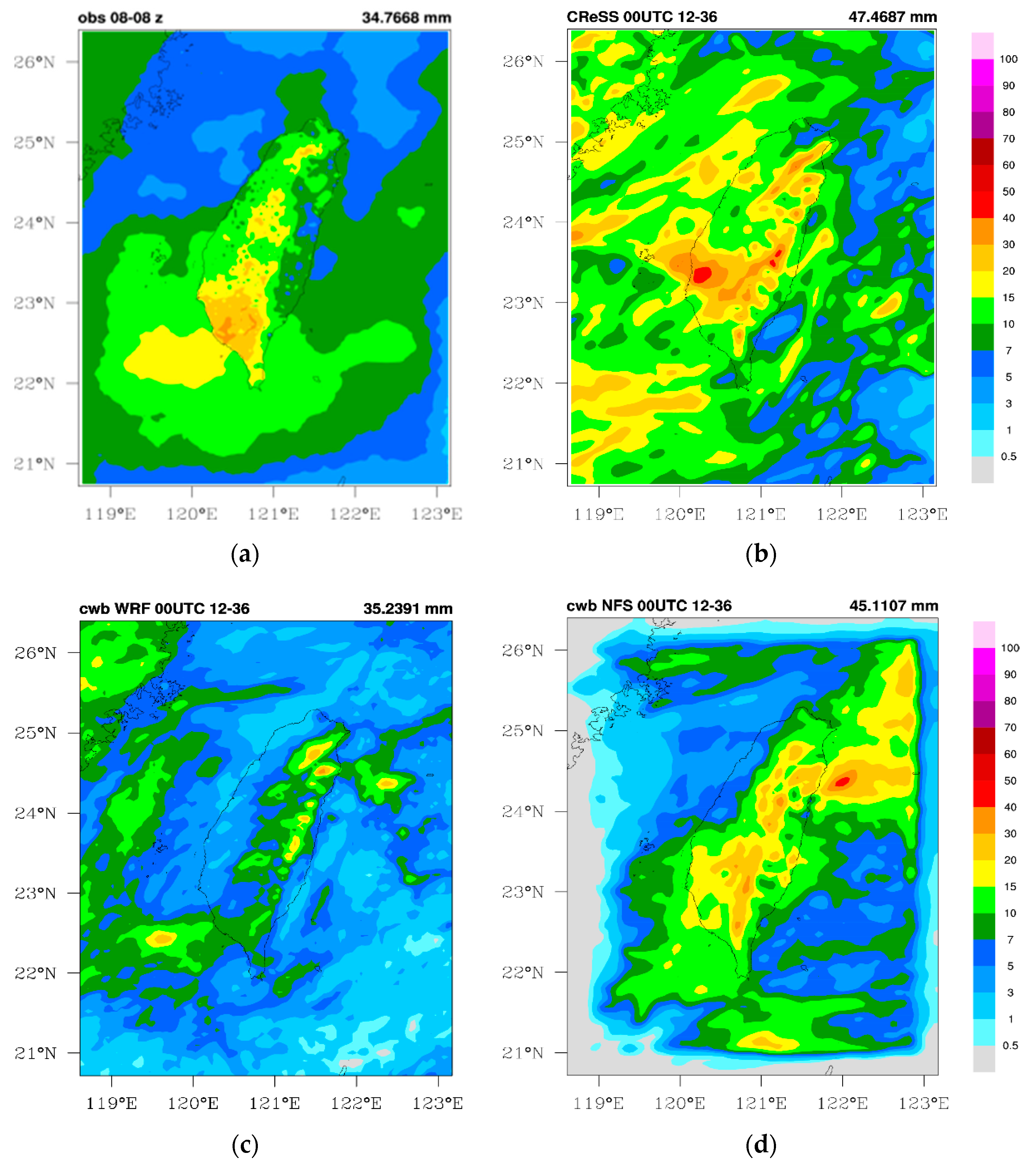
4.1. Distributions of Mean Daily Rainfall in the Season

The comparison between observed and model (CReSS, CWB WRF, CWB NFS) forecasted (0–24 h) mean daily rainfall distributions over Taiwan during the whole SoWMEX experiment period in 2008 (15 May–30 June) is presented in Figure 1. In the observation, with three major daily rainfall maxima in northern, central, and southern Taiwan near the northern slopes of the Snow Mountain Range (SMR) and along the western slopes of southern Central Mountain Range (CMR), the mountain areas received more rain than the low-lying plains on either side of the mountains. The rainfall was highest (34.77 mm) over the windward side in southern CMR in southern Taiwan (Figure 1a). Although with location errors, the mean rainfall distribution of CReSS model agreed moderately well with observations during 15 May–30 June (Figure 1b). Over prediction of Mei-yu seasonal rainfall over much of Taiwan, especially over CMR and SMR by CReSS was evident. In contrast, the CWB WRF exhibited a strong tendency of under-prediction of the mean daily rainfall, with an amount and amplitude too small over the topography (Figure 1c). The CWB NFS exhibited three distinct rainfall maxima over northern, central, and southern Taiwan with comparable rainfall amount, and resembled the observed data for the season quite well over the island (Figure 1d). The predicted maximum rainfall centers with the peak values up to about 37 mm were closer to the observation. However, the CWB NFS under predicted the mean rainfall over southwestern plains of Taiwan, in the South China Sea (SCS), and over much of the surrounding oceans (Figure 1d). The area shown in Figure 1 is roughly the verification area using the object-oriented method.

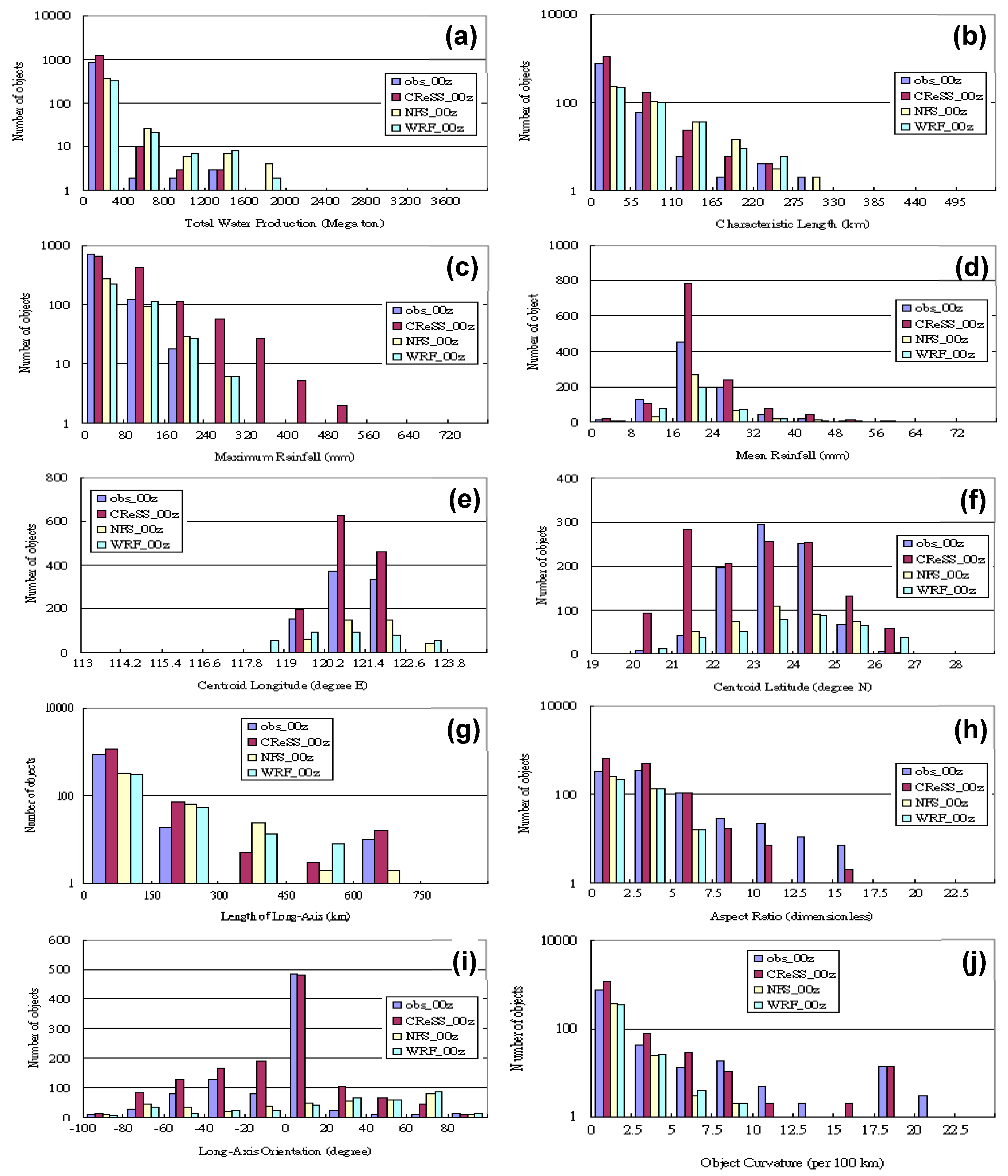
4.2. Object-Based Analysis for Model Forecasts at 0000 UTC

4.2.1. Statistics of Major Attributes of Rainfall Objects

Table 2 presents the mean value and standard deviation (SD) of major parameters and attributes of rainfall for objects in observation and the three model forecasts initialized daily at 0000 UTC. Compared to the observed number of objects (863), the CReSS (1287) produced roughly one-half too many while both WRF and NFS (~400) had about one-half too few. Combined with the information on object water output (production) and size, WRF and NFS tended to predict objects considerably larger than the observation with higher water output, although fewer in numbers. For example, at over 5500 km2, the mean object size in WRF and NFS was almost three times that in the observation (~1700 km2) and in CReSS (~2100 km2). In contrast, CReSS was the closest to the observation in object size, though with over prediction. However, the total water output from all objects in all three models (at 55.5–68.2 gigatons) exceeded significantly that in the observation (29.3 × 863 = 25.3 gigatons). This apparent discrepancy suggests that a much smaller fraction of the observed precipitation falls within the objects than the model rainfall. The SD values also indicate that the CReSS model is overall closer to the observation in rain object size. The mean rainfall amount of all objects in the four datasets were all very close (ranging from 20.7 to 22.7 mm), so the total amount for the entire season was very much dictated by the total number of objects, and thus over-prediction by CReSS and under-prediction by both WRF and NFS, in general agreement with Figure 1.
On the other hand, the maximum rainfall predicted suggests an overestimation by all three models, which is characteristic of convective-permitting models, but this might also have been influenced by the low resolution of the TRMM data, and even the comparatively lower resolution of the rain-gauge network than model grids. The overestimation in peak rainfall was more serious in CReSS, but not so at the 50-percentile (Table 2) and below (not shown). In the category of rainfall intensity, WRF and NFS also tended to have smaller SD values compared to observation, consistent with their underestimation problem. Judged from the averaged location of object centroid (center of mass), objects tended to be slightly south, toward the northeast, and east in CReSS, WRF, and NFS, respectively, compared to the observation (Table 2), also in rough agreement with Figure 1 for CReSS and NFS. In terms of object shape, the long axis orientation predicted by CReSS model (−6.6) was closer to observation (−9.4) than WRF and NFS with positive angles. With a greater number of smaller objects, the average lengths of long and short axes in CReSS were also closest to the observation (Table 2), but again tended to be too long in both WRF and NFS (with bigger objects).

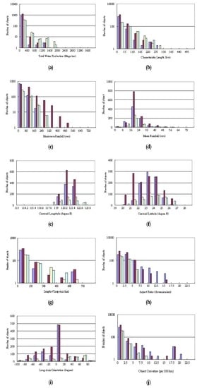
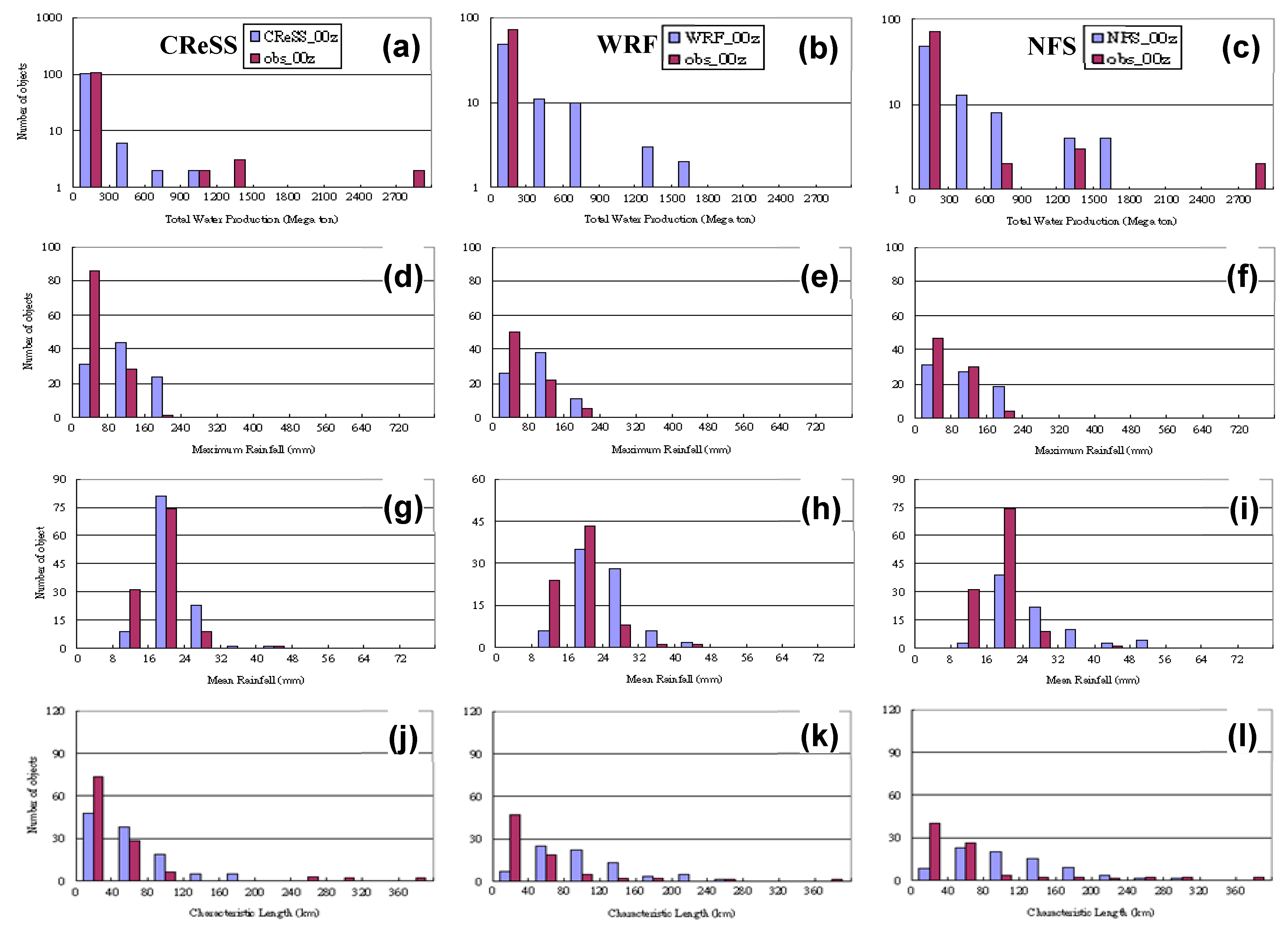
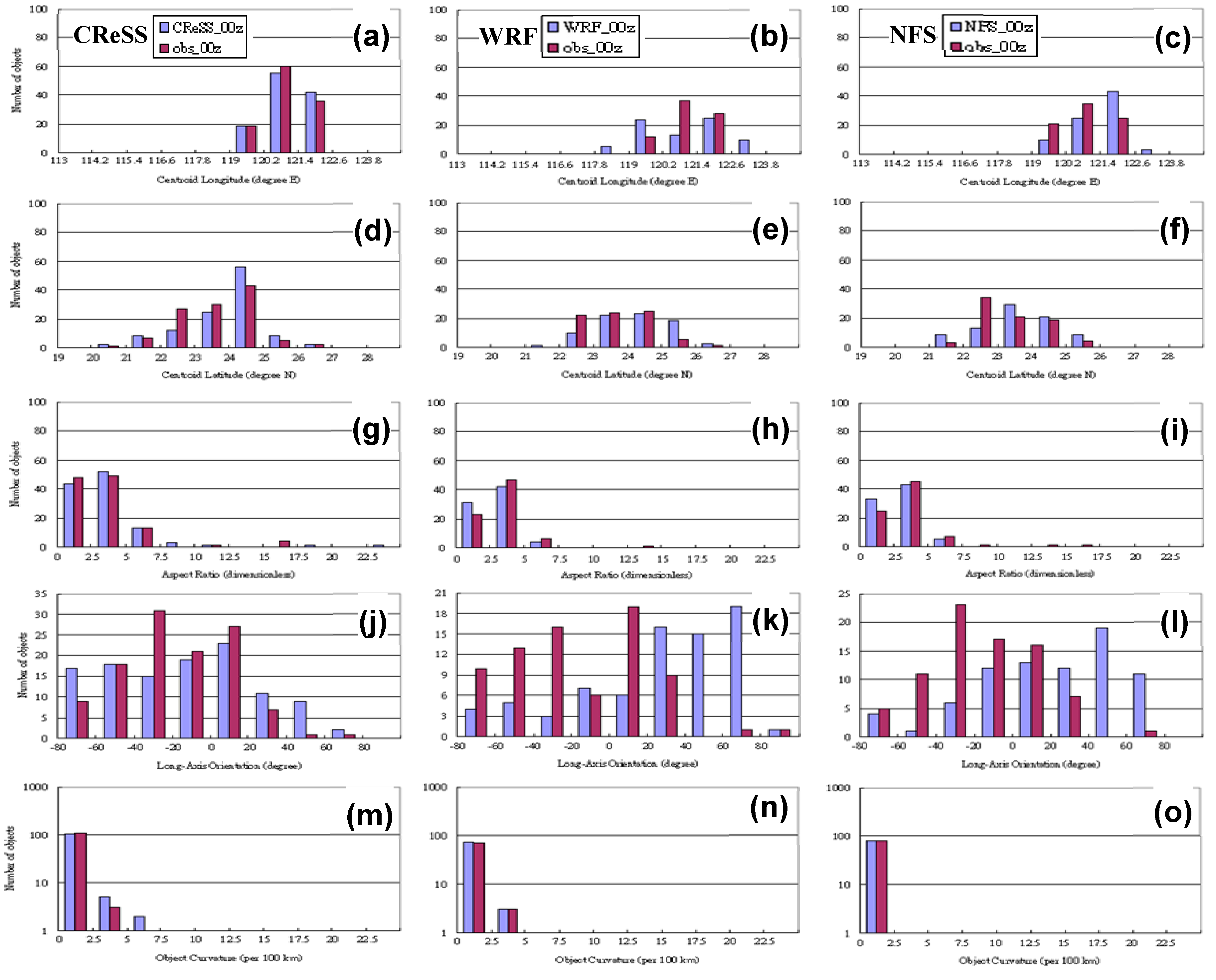
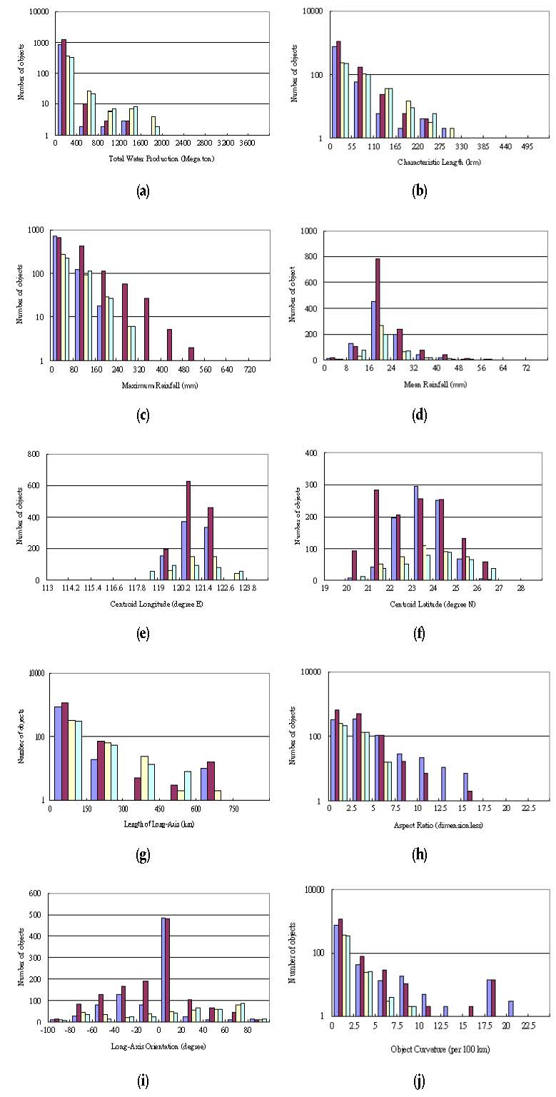
4.2.2. Distributions of Attribute Parameters of Rainfall Objects

In addition to the statistics (mean and SD), major attributes can be further compared between forecast and observed objects in their distributions. In a sense, these distributions represent the climatology of attributes that characterize several aspects (size, intensity, location, and shape, etc.) of rainfall objects during the data period. In this way, their similarity to observed objects can be assessed, and systematic model errors can be identified by the biases in the distributions. Furthermore, these kind of findings can be applied for improvement of weather and climate models.
In Figure 2, a number of object attributes are compared among the observation and the three models for their distribution, after stratification by their values. The total water production in all four datasets shows roughly a χ distribution (Figure 2a), with a large number of small objects and a rapid decrease in object number with increasing amount of total precipitation. The characteristic length, which is simply the square root of rain-object area, indicates a similar tendency (Figure 2b), while no object exceeded a length of 330 km. Thus, both attributes linked to object size indicate a larger number of smaller objects and a smaller number of bigger objects, even though they are stratified independently. At the characteristics length of 110–330 km, both WRF and NFS produced too many large objects (also those ≥1200 megatons), but too few objects in the lowest class (Figure 2a,b). On the other hand, the overestimation by CReSS was relatively less and confined in small-object groups below about 800 megatons in water production. The size information in Figure 2a,b was consistent with Table 2, but additional information regarding the distribution can be revealed. Overall, the size distribution of objects produced by CReSS was closer to observation than those by WRF and NFS.
The distribution of number of objects with respect to maximum rainfall shows that the CReSS model had a strong tendency to produce intense rainfall, even reaching ~500 mm (per 6 h) occasionally, but the observation did not exceed 240 mm (Figure 2c). Produced due to the high resolution of CReSS, such objects were most likely quite small in size (Figure 2a,b). Both WRF and NFS seemed to under-forecast objects when the maximum rainfall was lower (below 160 mm) and over-forecast when the maximum rainfall was higher, but the latter issue was not as serious as in CReSS. This result is in agreement with Table 2, which also reveals that the overestimation of maximum rainfall was highest for CReSS, as it produced more concentrated rainfall. This might be linked to the fact that CReSS did not use any CPS, which would have consumed some instability in the parent domain (15 km coarse grid) of WRF and NFS. The average rainfall values at 90, 75, and 50 percentiles in Table 2 also suggest that CReSS objects tended to exhibit larger variation in rainfall and less so in WRF and NFS, which tended to produce a smaller number of bigger objects with weaker intensity. The distribution of objects with respect to mean rainfall (Figure 2d) reveals that all three models had a normal-type distribution similar to observation, with a peak at 16–24 mm (cf. Table 2), except that the CReSS model had more, whereas NSF and WRF had fewer objects than the observation. Thus, the object number strongly dictates the difference here, and the CReSS exceeded observation by ~350 objects at 16–24 mm.
The distribution of centroid location (longitude and latitude) of observed objects exhibited high frequency at 120.2°–121.4° E and 23°–25° N, corresponding to the terrain of Taiwan and reflecting its influences (Figure 2e,f). The pattern of CReSS in latitudes exhibited higher frequency at 20°–22° N than observed, showing a tendency to produce rainfall objects too far to the south. Both NFS and WRF, on the other hand, were slightly prone to eastward and northward displacement, respectively.
Figure 2g–j show the dependence of object number on four shape- and orientation-related attributes. The observed distribution with long-axis length (Figure 2g) exhibited twin peaks, with the primary peak at 0–150 km (small objects) and a secondary peak at 600–750 km (big objects). Among the three models, the distribution in CReSS was closest to the observation with a similar pattern and two peaks at the correct length. In WRF and NFS, there was a lack of objects in the longest class of 600–750 km, where the objects were most likely associated with fronts. This tendency was also seen in the pattern with aspect ratio (Figure 2h), where the observation has the most objects with low aspect ratio (<2.5) and fewer ones toward higher ratio up to 15–17.5. Although all three models showed a similar decreasing pattern with aspect ratio, CReSS was the only one to produce objects with values between 7.5 and 17.5 (Figure 2h), and thus was also closest to the observation. For NFS and WRF, the aspect ratios of their objects were confined within 7.5, and thus tended to be rounder, not elongated in shape. This explains the lack of objects with longer axis for WRF and NFS in Figure 2g, also in agreement with Table 2.
In the parameter of long-axis orientation, the distribution pattern of CReSS agrees the best with the observation, with highest frequency at 0°–20° and alignments close to E–W direction (Figure 2i). There were also some objects with negative orientation (NW–SE) and fewer ones with orientation above 20° (NE–SW) in both observation and CReSS. However, in WRF and NFS, although their objects were more evenly distributed across the spectrum, more have positive orientation with highest frequency at 60°–80°, along a NNE–SSW direction (Figure 2i). For object curvature (or radius per 100 km), the distribution was again bi-modal and the pattern of CReSS best resembled the observation (Figure 2j), with the major peak at small curvature and a minor one at large curvature (17.5 − 20 × 10−2). On the contrary, both WRF and NFS had object curvatures below 10 × 10−2, i.e., with a radius >1000 km.
Overall, the objects produced by CReSS agree considerably better with the observation in their distributions in size, shape, and orientation, compared to CWB WRF and CWB NFS. However, CReSS also tended to produce an excessive number of small objects, often with high peak rainfall, although the mean rainfall distribution was reasonable. For NFS and WRF, their objects were about 50% too few, but some of them tended to be too large in size (Figure 2a,b and Table 2).

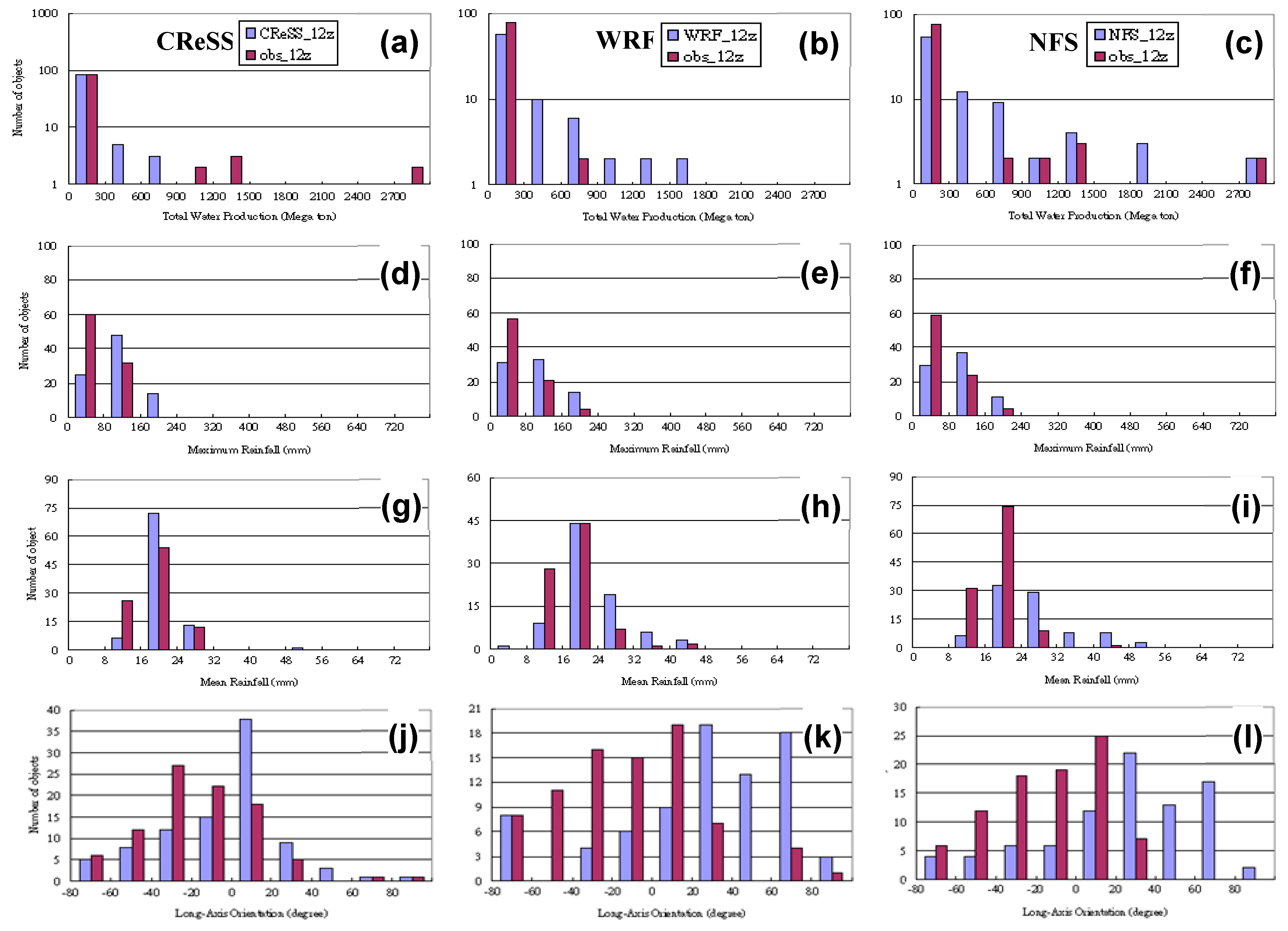
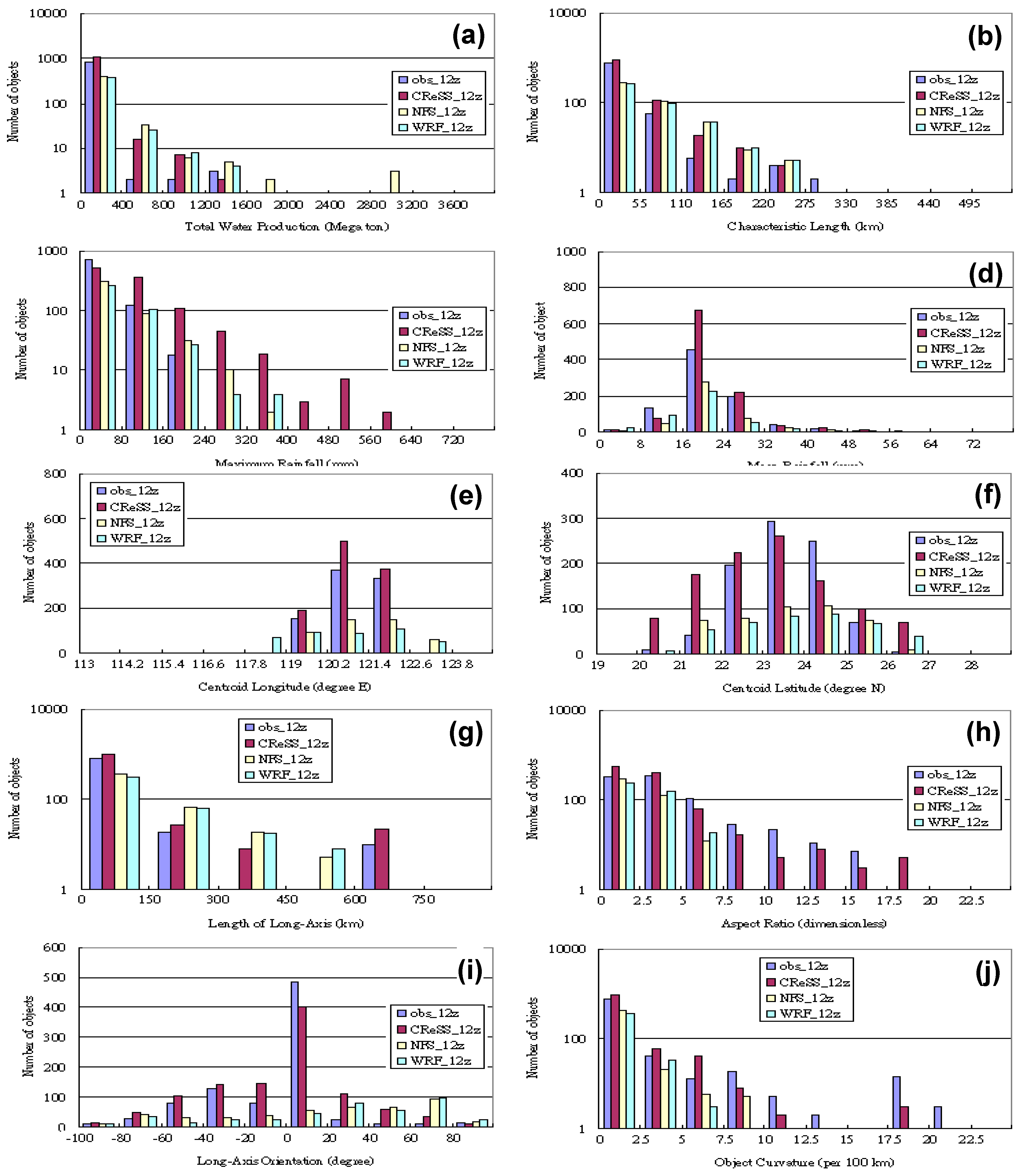
4.3. Object-Based Analysis for Model Forecasts at 1200 UTC

As for the 0000-UTC forecasts, the same object-oriented analysis was performed for the forecasts initialized at 1200 UTC each day during SoWMEX, also at the range of 12–36 h, and the results are presented in Table 3 and Figure 3. With 863, 1067, 408, and 448 objects in observation, CReSS, WRF, and NFS, following the order for 1200-UTC runs, the mean value and SD of various parameters and attributes were identical for the observation (Table 3), and also very similar to those in Table 2 for all models. However, compared to Table 2, some improvements were seen in CReSS in the number of objects (a reduction by 220), and the statistics produced by CReSS were also closest to the observed statistics in most of the attribute categories, except for peak rainfall intensity (and high percentile values) and centroid latitude (Table 3). In WRF and NFS, their object numbers also increased by roughly 10% (by 37 and 47, respectively) and improved to some extent.
Figure 3 presents the distribution of objects with respect to the value of attributes, for objects produced at the initial time of 1200 UTC, and naturally the model characteristics bear similarities to those of 0000 UTC (cf. Figure 2). The statistical distributions in Figure 3a–e are very similar to Figure 2a–e, suggesting the same features and differences, except that with fewer objects (1067), the patterns in mean rainfall and centroid longitude by CReSS now agree better with the observation in Figure 3d,e. For these attributes, except for maximum rainfall, the distributions in CReSS were in general closest to the observation although still with some overestimation in object numbers. In NFS and WRF, the low bias in object numbers was still evident since the improvement (by ~10%) was not as much.
More discernible improvements can be seen due to the change of initial time. Figure 3f shows that for 1200-UTC runs, the location error in the centroid of objects as depicted in Figure 2f has been improved in CReSS. The distribution was more to the south compared to the observation, with the highest frequency at 21–22° N in Figure 2f. However, in Figure 3f, the highest frequency now appears at 23–24° N as observed, correcting (or at least remedying) the location error.
Again, the distributions of objects in Figure 3g–j are in general similar to those produced by the forecasts at the initial time of 0000 UTC (Figure 2g–j). Overall, the CReSS simulation was closest to observation. Some improvements in performance of CReSS were also seen in the distribution of aspect ratio (Figure 3h), as well as in the alignment of object, again with most objects oriented in E–W and NNE–SSW direction, in association with the reduction in object number. In contrast, both WRF and NFS failed to catch the observed pattern, exhibiting more objects aligned in NW–SE direction and the highest frequency over 60°–80° N. Thus, the same distributions remained for most attributes, while some improvements were seen in some aspects.
The above improvements observed from an initial time of 0000 to 1200 UTC were most likely linked to the preferred timing of rainfall in the diurnal cycle in Taiwan. Many previous studies have shown that a strong diurnal cycle in rainfall exists in the Taiwan Mei-yu season, with more rainfall during local afternoon (roughly 0300-0900 UTC) and less rainfall at night [9,13,24,25,26]. Therefore, within the range of 12–36 h, the rainfall in the 1200-UTC runs (starting from 2000 LST) mainly occurs during 15–21 h under previously undisturbed conditions. The rainfall in 0000-UTC runs, on the other hand, occurs mainly during 27–33 h, which is during the second day and often time the atmosphere is already disturbed (on day 1). The shorter range and better conditions in the 1200-UTC runs were most likely the main causes of the difference in performance by all three models.

4.4. Object-Based Analysis for Matched Pairs between Observation and Forecast

Here in this subsection, the distributions of key object attributes of matched objects between the observation and each of the three model forecasts are compared, which is helpful in understanding the difference before and after matching, and if there is any improvement for matched pairs. An overall statistics of matched pairs is briefed in Table 4 for both initial times. It is revealed that the average values of total water volume, object size, length of long axis, maximum rainfall, long-axis length all increased significantly from those before matching (Table 4, cf. Table 2 and Table 3), while the curvature is lowered. These facts indicate that it is easier for larger objects to be paired successfully, as expected from the design of the matching procedure.
The distribution of number of objects with relevant parameters for matched objects between the observation and each of the three models at the initial time of 0000 UTC are presented in Figure 4 and Figure 5. The CReSS model agrees with the observation for objects with total water production near 0–300 megaton, where it had highest number of smaller objects (Figure 4a and Figure 5a). On the other hand, at the class of 0–300 megaton, both NFS and WRF had slightly fewer objects (Figure 4b,c) as their distributions of characteristics length also showed very few small objects (Figure 4k,l). However, above 300 megatons, all three models had more objects than the observation (Figure 4a–c). This is more evident in NFS and WRF and may arise from bigger objects, as models usually overestimate the number of objects that exceed 40 km in characteristics length (Figure 4j–l). Mean total water production was also significantly overestimated by the WRF and NFS models in Table 4. For maximum rainfall, as before matching, all models under-forecast the lighter rainfall below 80 mm and over-forecast the stronger rainfall above 80 mm for matched objects (Figure 4d–f). Table 4 also indicates that the maximum rainfall in CReSS was highest as compared to the other two models, pointing to more concentrated rainfall due to its higher resolution. However, even at 90 percentile, the rainfall decreased to a value much closer to observation (Table 4), though still higher than the latter (as also in WRF and NFS). The NFS agreed the best with the observation in the distribution of maximum rainfall among the three models (Figure 4f).
The distribution of mean 6 h rainfall indicates highest frequency of occurrence at 16–24 mm for observation as well as for CReSS, WRF, NFS (Figure 4g–i); thus, in general all three model’s patterns agreed with the observation, although their objects tended to have a higher mean rainfall (>24 mm) than observed. This overestimation in rainfall was more significant in NFS (cf. Table 4), and the pattern in CReSS was closest to the observed one, both with a narrow peak at 16–24 mm (Figure 4g). Compared to Figure 2d, which shows a much greater number of objects in CReSS than observed before matching, the overestimation by CReSS was corrected, because the numbers of objects were now the same after matching. By comparison, the agreement between the distribution in either WRF or NFS and the observed one was not as good as CReSS, in the case of matched objects. In the distribution of characteristic length after pairing, the observed objects had a χ distribution (Figure 4j–l), and again the distribution in CReSS was the closest to it. On the other hand, NFS and WRF did not follow a pattern like the observed data, as they lacked smaller objects but had too many bigger ones (above 80 km in characteristic length), in agreement with Table 4. Again, with the same number of objects (115) after matching, the over-estimation problem seen in CReSS in Figure 2b (before matching) is noticeably improved in Figure 4j.
The distributions of number of objects with respect to the value of attributes linked to location, orientation, and shape after matching are shown in Figure 5. The observed distribution of object centroid location (longitude and latitude) exhibited high frequency at 120.2°–121.4° E and 23°–25° N corresponding to the mountain range of Taiwan as before (Figure 5a–f). Since the matching procedure considers the distance between the two object candidates as a major criterion, the distributions in observed and model objects must be fairly close after matching. The pattern in CReSS seemed to be more concentrated in longitude (than the other models) as well as in latitude, with highest frequency at 24°–25° N in northern Taiwan (Figure 5a,d). Distributions in both NFS (Figure 5c,f) and WRF (Figure 5b,e) appeared more flat and across a wider range in centroid location, and there was a slight tendency in NFS to be more toward the northeast for objects in southern Taiwan (22°–24° N). Some of these results are also supported by the data in Table 4 (for 0000-UTC forecasts).
For parameters related to object shape, the distribution of aspect ratio was very close to the observation for each of the three models (Figure 5g–i). However, very few objects had an aspect ratio larger than 7.5, as they tended to be bigger objects, as revealed in Table 4. Again, even after matching, the distribution of long-axis orientation for CReSS was closest to observation (Figure 5j) and most matched objects were found to have an alignment angle less than 20° or negative, i.e., oriented in nearly E–W and NW–SE direction (also Table 4). In the case of NFS and WRF, their objects paired with the observation tended to exhibit positive orientation angle (in NE–SW direction), i.e., shifted toward the right side (Figure 5k,l), but more objects were of negative angle in the observation. However, since the matched objects tended to have larger size and small aspect ratios, their shape was also less elongated (cf. Table 4), so the long-axis orientation may have been less important. Finally, for object curvature, all three models were very successful in producing the same distribution as observed (Figure 5m–o). However, the curvature of all paired objects tended to be small and below 7.5 × 10⁻², consistent with the characteristics of bigger objects and the results above.
The results for the paired objects between the observation and model forecasts at the initial time of 1200 UTC are shown in Table 4 in parentheses and Figure 6 for selected attributes. For runs at 1200 UTC, the statistics in Table 4 reveal results very similar to their counterparts at 0000 UTC. The distributions of total water production, maximum rainfall and mean rainfall (Figure 6a–i), likewise, highly resemble those at 0000 UTC (Figure 4a–i). For the patterns of long-axis orientation, which were quite different among the three models in Figure 5j–l, the same characteristics also remained for runs at 1200 UTC (Figure 6j–l), except perhaps that the CReSS objects now show a distribution closer to normal and centered at 0°–20°.

5. Conclusions

Following Part II [6], in which the development of an object-based rainfall verification method suitable for Taiwan is described, this work further applies the method to explore and understand the relative merit of three models: CReSS, CWB WRF, and CWB NFS, in the prediction of Mei-yu rainfall during SoWMEX experiment in 2008. Thus, the aim was different in the present study from Part II [6]. The models had a grid size of 3.5 to 5 km and the 0000 and 1200-UTC forecasts at the range of 12–36 h were used, so the rainfall data at each initial time formed a continuous time series. Accumulated into 6 h intervals, the data were then verified against the observation formed by merging CWB rain-gauge data with TRMM (3B42) data, for the NFS 5 km domain using the object-oriented method. In a parallel paper (Part I [7]), the subjective method was used, so the two methods complement each other. However, the object-oriented verification, as a different approach, is both useable and useful, and the differences in the performance of the models can be summarized as follows:
  • A total of 863 rainfall objects are identified for the 47-day period in observation, and CReSS produces over a thousand (about 200–400 more) while WRF and NFS have roughly 370–450 objects in the two initial times. The overall results from the mean, SD, and distributions of attribute parameters suggest that all three models show a tendency to over-forecast heavy rain and under-forecast light rain. The CReSS has about 25–50% too many objects and a strong tendency to produce small objects with more concentrated rainfall, but its total water production is the closest to the observation and the most reasonable. Both WRF and NFS, with only about one-half the total number of objects as observed, on the other hand, have a clear tendency to under forecast rainfall object number. Their objects tend to be larger in size but smaller in curvature, with less intense precipitation but high total water output compared to observation. The smaller rainfall objects in CReSS might be linked to its lack of a CPS, which would consume some instability in the environment in the parent domain in the case of WRF and NFS (in which a CPS is also turned off in the fine domain).
  • In all three model simulations, their object centroids exhibit higher frequency over the terrain of Taiwan, and this response to topography is very much understandable. Nonetheless, the CReSS model exhibits a tendency to simulate the rainfall slightly too south, and NFS and WRF slightly east and north to northwest, respectively, as interpreted from the distribution of the object centroid location. The shape-related and orientation attributes suggest that CReSS simulation is very much comparable to observation, especially for orientation aspect where most objects are found to align along N–E to NW–SE direction in both CReSS and observation. On the other hand, more NE–SW aligned objects appear in WRF and NFS.
  • Consistent with the design of the matching procedure between observed and modeled objects, larger objects with more water outputs are more easily matched. The over-estimation bias in size for bigger objects and under-estimation bias for smaller objects in NFS and WRF remains evident in matched pairs. A similar overestimation problem in CReSS in unmatched objects is noticeably improved in matched pairs. The total matched pairs, however, are few such that statistical significance of their attribute distributions is lowered. The reason for the low matching rate remains to be investigated and clarified in the future.
  • The number of objects and the distributions of some attributes were improved in all three models in the forecasts initialized at 1200 UTC, as compared to those at 0000 UTC, particular in CReSS also in terms of centroid location and alignment of objects. This is mainly attributable to the difference in the preferred timing of rainfall in Taiwan (in local afternoon) in the 12–36 h forecast range, which is within day 1 for 1200-UTC forecasts but on the second day for 0000-UTC ones.
The findings of this paper in general agree with those in Part I [7] where the focus is on subjective verification. Both the two analyses conclude that (i) the CReSS model performed more skillfully but with the over-forecasting and location error problem, and (ii) both NFS and WRF have an under-forecasting problem. However, model errors in some attributes like areal size, alignment, shape, and even internal structure (as inferred from rainfall at different percentiles) are difficult to assess except using an object-oriented approach. Therefore, the analysis like the present study offers a different and useful set of information on model performance, which can complement and support subjective or traditional objective verification methods [7,26]. With the highest resolution, the CReSS model comes out as best performing model in simulation the precipitation in the present study. On the other hand, NFS and WRF are close to each other but with somewhat worse skills. This result partially differs from the conclusion in Part I [7], where relative merits in each model are found through subjective comparison (e.g., CReSS in seasonal and diurnal variations, WRF in its stability, and NFS in overall spatial pattern of rainfall). Finally, it is evident that no single verification method is enough to cover all aspects of model QPFs and reach a concrete conclusion, so they should be used in combination for a more complete understanding.

Author Contributions

All authors contributed equally. All authors have read and agreed to the published version of the manuscript.

Funding

This research received no external funding.

Acknowledgments

The authors wish to thank the reviewers for their valuable comments and suggestions. The help from Huang, Y.-W., Wang, Y.-W., and Huang, S.-Y. is acknowledged. This research is supported by the Ministry of Science and Technology of Taiwan (grant numbers NSC 97-2625-M-003-004, NSC 97-2111-M-003-005-MY2, NSC 98-2625-M-003-002, MOST 105-2811-M-003-027, MOST 107-2811-M-003-520, MOST 108-2111-M-003-005-MY2, and MOST 108-2625-M-003-001) and by the Korea Meteorological Institute under Grant KMI 2018-05410.

Conflicts of Interest

The authors declare no conflict of interest.

References

  1. Gartner, W.E.; Baldwin, M.E.; Junker, N.W. Regional analysis of quantitative precipitation forecast from NCEP’s “Early”Eta and meso-Eta models. In Proceedings of the 16th Conference on Weather Analysis and Forecasting, Phonenix, AZ, USA, 11–16 January 1998; pp. 187–188. [Google Scholar]
  2. Ebert, E.E.; McBride, J.L. Verification of precipitation in weather systems: Determination of systematic errors. J. Hydrol. 2000, 239, 179–202. [Google Scholar] [CrossRef]
  3. Murphy, A.H. What is a good forecast? An essay on the nature of goodness in weather forecasting. Weather Forecast. 1993, 8, 281–293. [Google Scholar] [CrossRef] [Green Version]
  4. Davis, C.; Brown, B.; Bullock, R. Object-based verification of precipitation forecasts. Part I: Methodology and application to mesoscale rain areas. Mon. Weather Rev. 2006, 134, 1772–1784. [Google Scholar] [CrossRef] [Green Version]
  5. Davis, C.; Brown, B.; Rullock, R. Object-based verification of precipitation forecasts. Part II: Application to convective rain systems. Mon. Weather Rev. 2006, 134, 1785–1795. [Google Scholar] [CrossRef] [Green Version]
  6. Wang, C.C.; Paul, S.; Lee, D.I. Evaluation of rainfall forecasts by three mesoscale models during the Mei-yu season of 2008 in Taiwan. Part II: An object-oriented precipitation forecast verification method development. Atmosphere. under review.
  7. Paul, S.; Wang, C.C.; Tseng, L.S.; Lee, D.I. Evaluation of rainfall forecasts by three mesoscale models during the Mei-yu season of 2008 in Taiwan. Part I: Subjective comparison. Asia-Pasific J. Atmos. Sci. under review.
  8. Hsu, J. ARMTS up and running in Taiwan. Väisälä News 1998, 146, 24–26. [Google Scholar]
  9. Chen, T.C.; Yen, M.C.; Hsieh, J.C.; Arritt, R.W. Diurnal and seasonal variations of the rainfall measured by the Automatic Rainfall and Meteorological Telemetry System in Taiwan. Bull. Amer. Meteor. Soc. 1999, 80, 2299–2312. [Google Scholar] [CrossRef] [Green Version]
  10. Wang, C.C.; Kuo, H.C.; Yeh, T.C.; Chung, C.H.; Chen, Y.H.; Huang, S.Y.; Wang, Y.W.; Liu, C.H. High-resolution quantitative precipitation forecasts and simulations by the Cloud-Resolving Storm Simulator (CReSS) for Typhoon Morakot (2009). J. Hydrol. 2013, 506, 26–41. [Google Scholar] [CrossRef]
  11. Huffman, G.J.; Adler, R.F.; Bolvin, D.T.; Gu, G.; Nelkin, E.J.; Bowman, K.P.; Hong, Y.; Stocker, E.F.; Wolff, D.B. The TRMM Multisatellite Precipitation Analysis (TMPA): Quasi-global, multiyear, combined-Sensor precipitation estimates at fine scales. J. Hydrometeorl. 2007, 8, 38–55. [Google Scholar] [CrossRef]
  12. Cressman, G.P. An operational objective analysis system. Mon. Weather Rev. 1959, 87, 367–374. [Google Scholar] [CrossRef]
  13. Jou, B.J.D.; Lee, W.C.; Johnson, R.H. An overview of SoWMEX/TiMREX. In The Global Monsoon System: Research and Forecasts, 2nd ed.; Chang, C.-P., Ed.; World Scientific: Singapore, 2011; pp. 303–318. [Google Scholar]
  14. Tsuboki, K.; Sakakibara, A. Large-scale parallel computing of cloud resolving storm simulator. In High Performance Computing; Zima, H.P., Ed.; Springer: Berlin/Heidelberg, Germany, 2002; pp. 243–259. [Google Scholar]
  15. Tsuboki, K.; Sakakibara, A. Numerical Prediction of High-Impact Weather Systems. In The Textbook for Seventeenth IHP Training Course; HyARC; Nagoya University; UNESCO: Nagoya, Japan, 2007; 273p. [Google Scholar]
  16. Zhao, Q.; Black, T.L.; Baldwin, M.E. Implementation of the cloud prediction scheme in the Eta model at NCEP. Weather Forecast. 1997, 12, 697–713. [Google Scholar] [CrossRef]
  17. Detering, H.W.; Etling, D. Application of the Eε turbulence model to the atmosphere boundary layer. Bound. Layer Meteorol. 1985, 33, 113–133. [Google Scholar] [CrossRef]
  18. Segami, A.; Kurihara, K.; Nakamura, H.; Ueno, M.; Takano, I.; Tatsumi, Y. Operational mesoscale weather prediction with Japan Spectral Model. J. Meteorol. Soc. Jpn. 1989, 64, 637–664. [Google Scholar]
  19. Davies, R.; Randall, D.A.; Corsetti, T.G. A fast radiative parameterization for atmospheric circulation models. J. Geophys. Res. 1987, 92, 1009–1016. [Google Scholar]
  20. Skamarock, W.C.; Klemp, J.B.; Dudhia, J.; Gill, D.O.; Barker, D.M.; Wang, W.; Powers, J.G. A description of the Advanced Research WRF version 2. In NCAR Technical Note TN-468+STR; University Corporation for Atmospheric Research: Boulder, CO, USA, 2005; 100p. [Google Scholar]
  21. Hong, J.S. The evaluation of typhoon track and quantitative precipitation forecasts of CWB’s NFS in 2001. Meteor. Bull. 2002, 44, 41–53. [Google Scholar]
  22. Wang, C.C.; Huang, H.L.; Li, J.L.; Leou, T.M.; Chen, G.T.J. An evaluation on the performance of the CWB NFS model in the prediction of warm-season rainfall distribution and propagation over the East Asian continent. Terr. Atmos. Ocean. Sci. 2011, 22, 49–69. (In Chinese) [Google Scholar] [CrossRef] [Green Version]
  23. Ritter, G.X.; Wilson, J.N. Computer Vision Algorithms in Image Algebra; CRC Press: Boca Raton, FL, USA, 2001; 417p. [Google Scholar]
  24. Ruppert, J.H., Jr.; Johnson, R.H.; Rowe, A.K. Diurnal circulations and rainfall in Taiwan during SoWMEX/TiMREX (2008). Mon. Weather Rev. 2013, 141, 3851–3872. [Google Scholar] [CrossRef] [Green Version]
  25. Wang, C.C.; Hsu, J.C.S.; Chen, G.T.J.; Lee, D.I. A study of two propagating heavy-rainfall episodes near Taiwan during SoWMEX/TiMREX IOP-8 in June 2008. Part II: Sensitivity tests on the roles of synoptic conditions and topographic effects. Mon. Weather Rev. 2014, 142, 2644–2664. [Google Scholar] [CrossRef]
  26. Wang, C.C.; Chien, F.C.; Paul, S.; Lee, D.I.; Chuang, P.Y. An evaluation of WRF rainfall forecasts in Taiwan during three mei-yu seasons of 2008–2010. Weather Forecast. 2017, 32, 1329–1351. [Google Scholar] [CrossRef]
Figure 1. (a) Observed and predicted mean daily rainfall (mm, 0000–2400 UTC) distributions over Taiwan by the three models: (b) Cloud-Resolving Storm Simulator (CReSS), (c) Central Weather Bureau (CWB) Weather Research and Forecasting (WRF), and (d) CWB Non-hydrostatic Forecast System (NFS), during the period of South-West Monsoon Experiment (SoWMEX), from 15 May to 30 June 2008. The model initial time is 0000 UTC, at the range of 12–36 h. The maximum amount is given at the right side above each panel.
Atmosphere 11 00705 g001
Figure 2. The distribution of number of objects as a function of (a) total water production (megaton), (b) object characteristic length (km), (c) object maximum rainfall (mm), (d) object average rainfall (mm), (e) centroid longitude (° E), (f) centroid latitude (° N), (g) long-axis length (km), (h) aspect ratio (dimensionless), (i) long-axis orientation (degree), and (j) object curvature (radius per 100 km) in observation and (12–36 h) forecasts by the three models: CReSS, CWB NFS, and CWB WRF initialized at 0000 UTC during SoWMEX. At accumulation period every 6 h, a total of 863 objects are identified in observation, and there are 1287, 371, and 401 objects in forecasts by CReSS, WRF, and NFS, respectively. In panels (ac,g,h,j), the logarithmic scale is used in the vertical axis.
Atmosphere 11 00705 g002
Figure 3. As in Figure 2 (aj) but for (12–36 h) forecasts initialized daily at 1200 UTC. A total of 863, 1067, 408, and 448 objects are identified in observation, CReSS, WRF, and NFS, respectively.
Atmosphere 11 00705 g003
Figure 4. The distribution of number of matched objects as a function of (ac) total water production (megaton), (df) object maximum rainfall (mm), (gi) object average rainfall (mm), and (jl) characteristic length (km) between the observation and each of the three model forecasts initialized at 0000 UTC at the range of 12–36 h: CReSS (left column), WRF (central column), and NFS (right column). The number of objects successfully paired with observation is 115, 77, and 81, respectively, for CReSS, WRF, and NFS. In panels (ac), the logarithmic scale is used in the vertical axis. Note that in panels (a) and (h), the scale in vertical axis is different from others.
Atmosphere 11 00705 g004
Figure 5. As in Figure 4 but for (ac) centroid longitude (° E), (df) centroid latitude (° N), (gi) aspect ratio (dimensionless), (jl) long-axis orientation (degree), and (mo) object curvature (radius per 100 km), respectively. In panels (mo), the logarithmic scale is used in the vertical axis. Note that in panels (jl), the scales in vertical axis are different.
Atmosphere 11 00705 g005
Figure 6. (ai) As in Figure 4a–i and (jl) as in Figure 5m–o, but for (12–36 h) forecasts initialized daily at 1200 UTC. The number of objects successfully paired with observation is 92, 82, and 87, respectively, for CReSS, WRF, and NFS. Note that in some panels, the scales in vertical axis are different.
Atmosphere 11 00705 g006
Table 1. Fine-domain configuration and the major physical packages used in the CReSS (version 2.2), CWB WRF (version 2.2.1), and CWB NFS Model.
ModelCReSSCWB WRFCWB NFS
Grid size3.5 km5 km (domain 3)5 km (domain 3)
Grid dimension (x, y, z)330 × 280 × 40140 ×178 × 4591 × 121 × 30
Fine domain region113.5°–124.5° N, 19°–28° N117°–125° N, 20°–28.5° N118.7°–123.3° N, 20.8°–26.4° N
Cloud microphysicsBulk cold-rain (six species)NASA GoddardSimple ice [16]
Cumulus parameterizationNoneNoneNone
PBL parameterization1.5-order closure with TKE predictionYonsei University[17]
Radiation parameterization[18]RRTM and Goddard[19]
Table 2. Mean value and standard deviation (SD) of major parameters and attributes of rainfall objects in observation, and CReSS, CWB WRF, and CWB NFS forecasts initialized at 0000 UTC. The model forecast range used is 12–36 h, and SD values are given in parentheses.
ParameterObservationCReSSCWB WRFCWB NFS
Mean (SD)Mean (SD)Mean (SD)Mean (SD)
Total object number8631287371401
Water production (106 ton)29.3 (166.9)44.2 (120.1)149.6 (285.6)170.1 (379.3)
Area size (km2)1692.8 (9432.9)2071.1 (5529.9)5674.9 (9584.4)5871.4 (10,056.6)
Mean rainfall (mm)21.9 (8.2)22.7 (7.9)20.7 (7.0)21.7 (7.2)
Maximum rainfall (mm)48.5 (36.9)99.6 (77.2)80.7 (63.6)74.5 (56.3)
90-percentile rainfall (mm)37.1 (18.1)58.5 (24.3)45.4 (22.1)45.6 (21.2)
75-percentile rainfall (mm)29.9 (11.4)34.5 (11.6)29.4 (10.2)30.6 (10.5)
50-percentile rainfall (mm)20.1 (13.5)13.4 (15.3)16.6 (5.3)18.0 (4.9)
Centroid longitude (° E)121.05 (0.79)120.95 (2.47)120.61 (3.40)121.25 (0.98)
Centroid latitude (° N)23.66 (1.06)23.23 (1.57)23.94 (1.54)23.67 (1.32)
Long-axis orientation (°)−9.4 (27.0)−6.6 (34.0)21.8 (48.2)12.6 (49.8)
Long-axis length (km)42.8 (74.2)64.8 (85.3)104.9 (98.4)105.6 (100.6)
Short-axis length (km)13.7 (24.3)21.0 (44.8)37.4 (26.0)38.3 (26.5)
Aspect ratio3.6 (2.7)3.0 (1.9)2.6 (1.1)2.5 (1.1)
Curvature (10−2)1.36 (3.93)1.07 (2.61)0.81 (1.40)0.69 (1.21)
Table 3. As in Table 2 but showing the results for observation and model forecasts corresponding to the initial time of 1200 UTC.
ParameterObservationCReSSCWB WRFCWB NFS
Mean (SD)Mean (SD)Mean (SD)Mean (SD)
Total object number8631067408448
Water production (106 ton)29.3 (166.9)48.9 (142.1)158.5 (387.4)155.6 (354.6)
Area size (km2)1692.8 (9432.9)2146.8 (5956.7)5966.4 (11,945.4)5258.6 (9711.8)
Mean rainfall (mm)21.9 (8.2)22.3 (7.7)19.2 (7.0)22.0 (7.9)
Maximum rainfall (mm) 48.5 (36.9)105.1 (85.5)74.9 (58.8)75.4 (62.1)
90-percentile rainfall (mm)37.1 (18.1)62.8 (27.1)41.5 (20.2)45.9 (23.7)
75-percentile rainfall (mm)29.9 (11.4)35.0 (12.5)27.0 (10.0)30.6 (11.4)
50-percentile rainfall (mm)20.1 (13.5)11.1 (14.4)15.8 (5.0)18.1 (5.3)
Centroid longitude (° E)121.05 (0.79)120.92 (1.98)120.76 (1.42)121.26 (1.05)
Centroid latitude (° N)23.66 (1.06)23.28 (1.53)23.85 (1.53)23.63 (1.38)
Long-axis orientation (°)−9.4 (27.0)−4.4 (33.9)23.1 (48.4)17.2 (48.8)
Long-axis length (km)42.8 (74.2)65.1 (94.4)104.4 (105.2)94.9 (94.0)
Short-axis length (km)13.7 (24.3)20.0 (16.5)35.7 (28.0)36.1 (26.9)
Aspect ratio3.6 (2.7)3.1 (2.2)2.7 (1.1)2.4 (1.0)
Curvature (10−2)1.36 (3.93)1.00 (1.99)0.77 (1.12)0.80 (1.44)
Table 4. Mean value of major parameters and attributes of rainfall objects in observation, and CReSS, CWB WRF, and CWB NFS forecasts initialized at 0000 UTC after matching. The values for 1200-UTC forecasts are also shown (in parentheses). For the initial time of 0000 (1200) UTC, the number of matched objects are 115, 77 and 81 (92, 82 and 87) for CReSS, WRF, and NFS, respectively. For the observation, the values for matched objects with CReSS are shown.
ParameterObservationCReSSCWB WRFCWB NFS
Initial time (UTC)0000 (1200)0000 (1200)0000 (1200)0000 (1200)
Total object number115 (92)115 (92)77 (82)81 (87)
Water production (106 ton)127.7 (152.9)113.8 (92.7)365.1 (393.3)484.3 (452.5)
Area size (km2)7447.9 (8921.9)5279.4 (4413.7)13,709.1 (13,664.3)14,971.6 (13,642.8)
Mean rainfall (mm)18.7 (18.5)21.2 (20.9)23.9 (23.0)26.4 (26.9)
Maximum rainfall (mm) 68.3 (69.2)139.1 (124.4)111.7 (112.3)119.2 (123.4)
90-percentile rainfall (mm)44.8 (43.4)63.4 (68.6)51.9 (49.8)57.4 (60.3)
75-percentile rainfall (mm)31.9 (30.3)35.0 (36.8)32.8 (31.5)36.2 (37.1)
50-percentile rainfall (mm)11.0 (12.5)5.9 (5.1)18.4 (17.9)20.0 (19.7)
Centroid longitude (° E)120.97 (120.87)121.04 (120.98)120.88 (120.62)121.39 (121.34)
Centroid latitude (° N)23.70 (23.66)23.91 (23.87)24.21 (23.92)23.63 (23.55)
Long-axis orientation (°)−19.4 (−19.0)−16.0 (−3.2)25.0 (22.1)17.0 (22.5)
Long-axis length (km)100.0 (106.3)134.7 (121.4)187.1 (172.6)194.5 (178.4)
Short-axis length (km)30.5 (36.8)34.8 (27.6)62.3 (57.3)64.6 (60.3)
Aspect ratio 3.6 (3.1)3.7 (3.9)3.0 (2.9)2.9 (2.8)
Curvature (10−2) 0.61 (0.73)0.60 (0.74)0.41 (0.41)0.27 (0.33)

