Tropical Atlantic Mixed Layer Buoyancy Seasonality: Atmospheric and Oceanic Physical Processes Contributions

 , and
, and 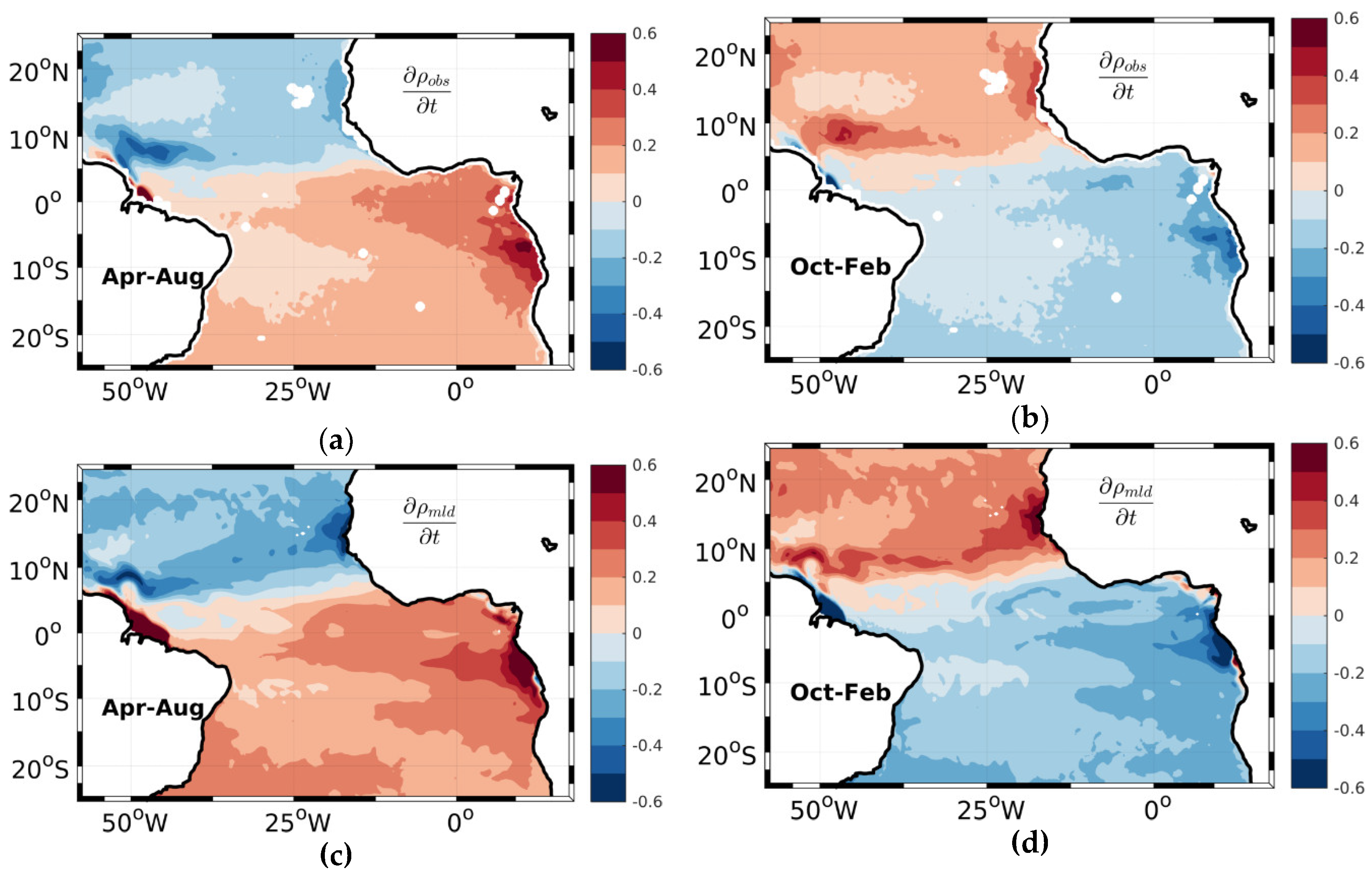
Abstract
1. Introduction
2. Model and Methodology
2.1. Model Description
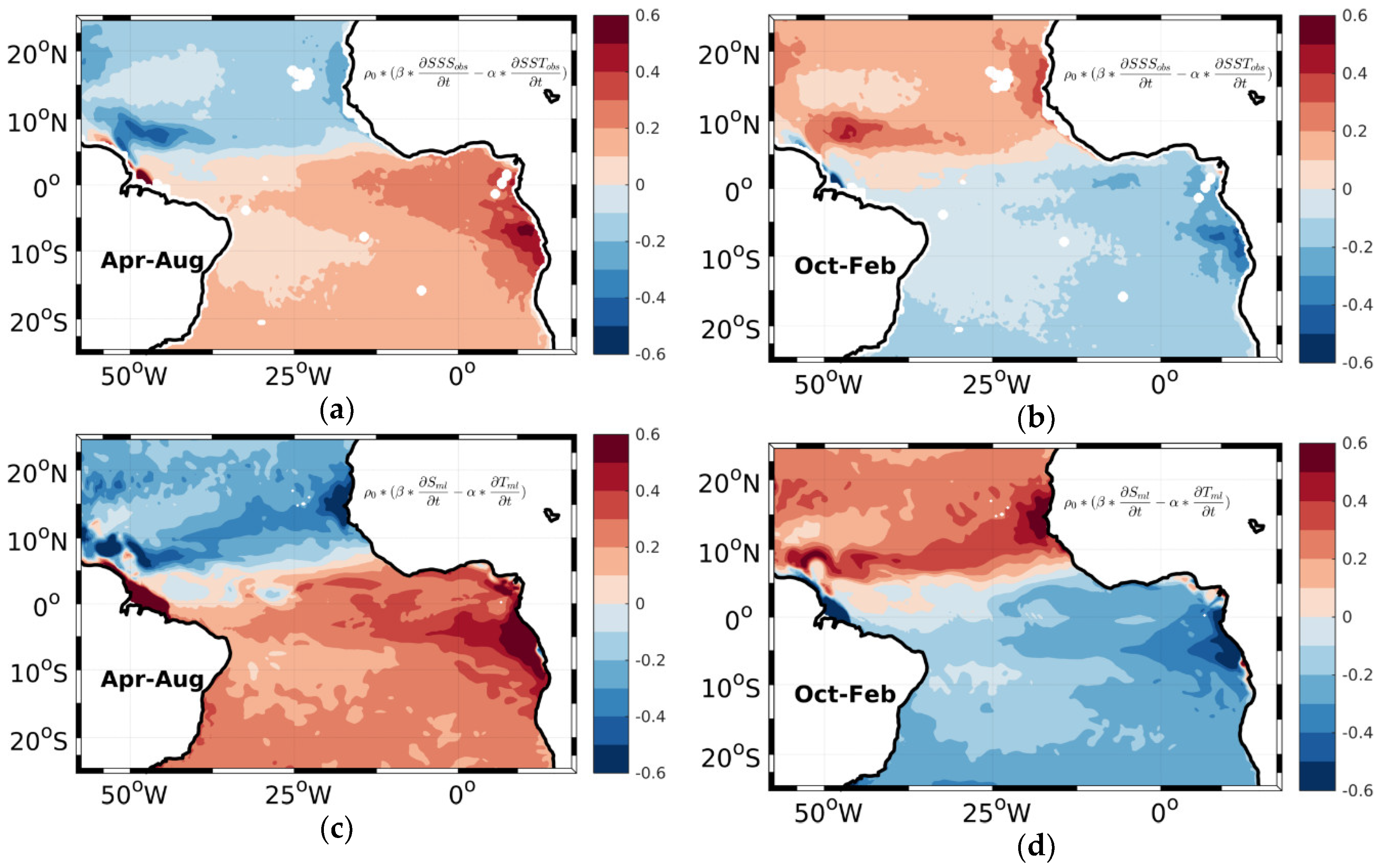
2.2. Density as a Function of Temperature and Salinity
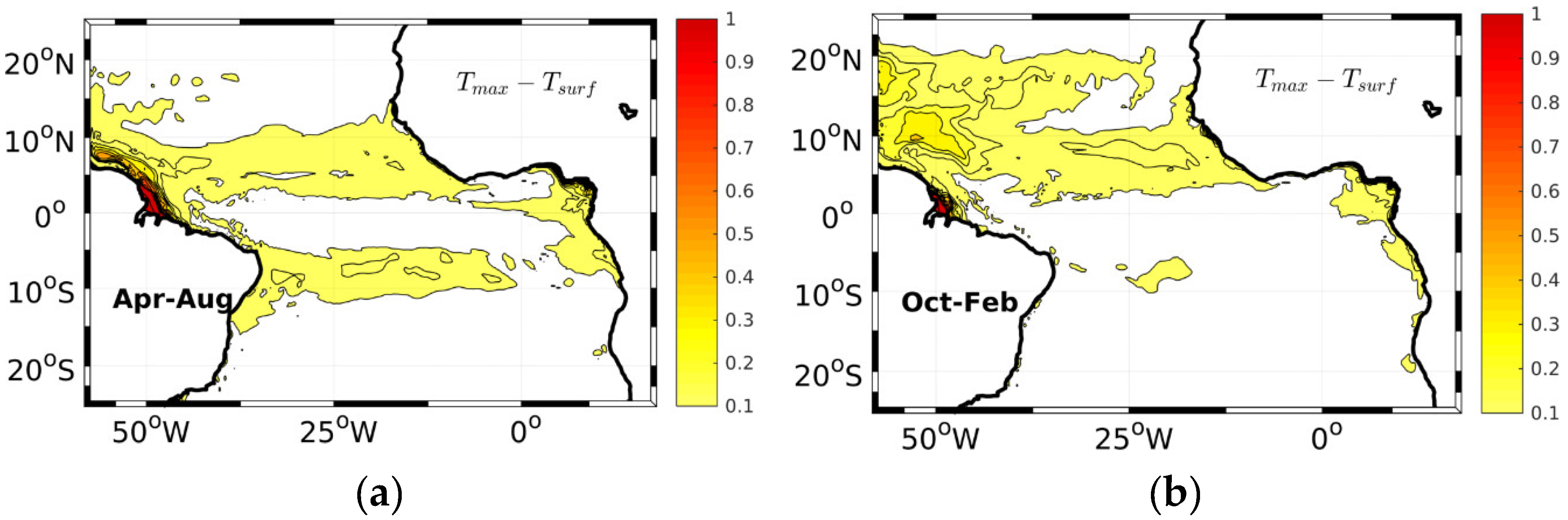
2.3. Mixed Layer Density: Model-Observation Comparison and Linearization
3. Results
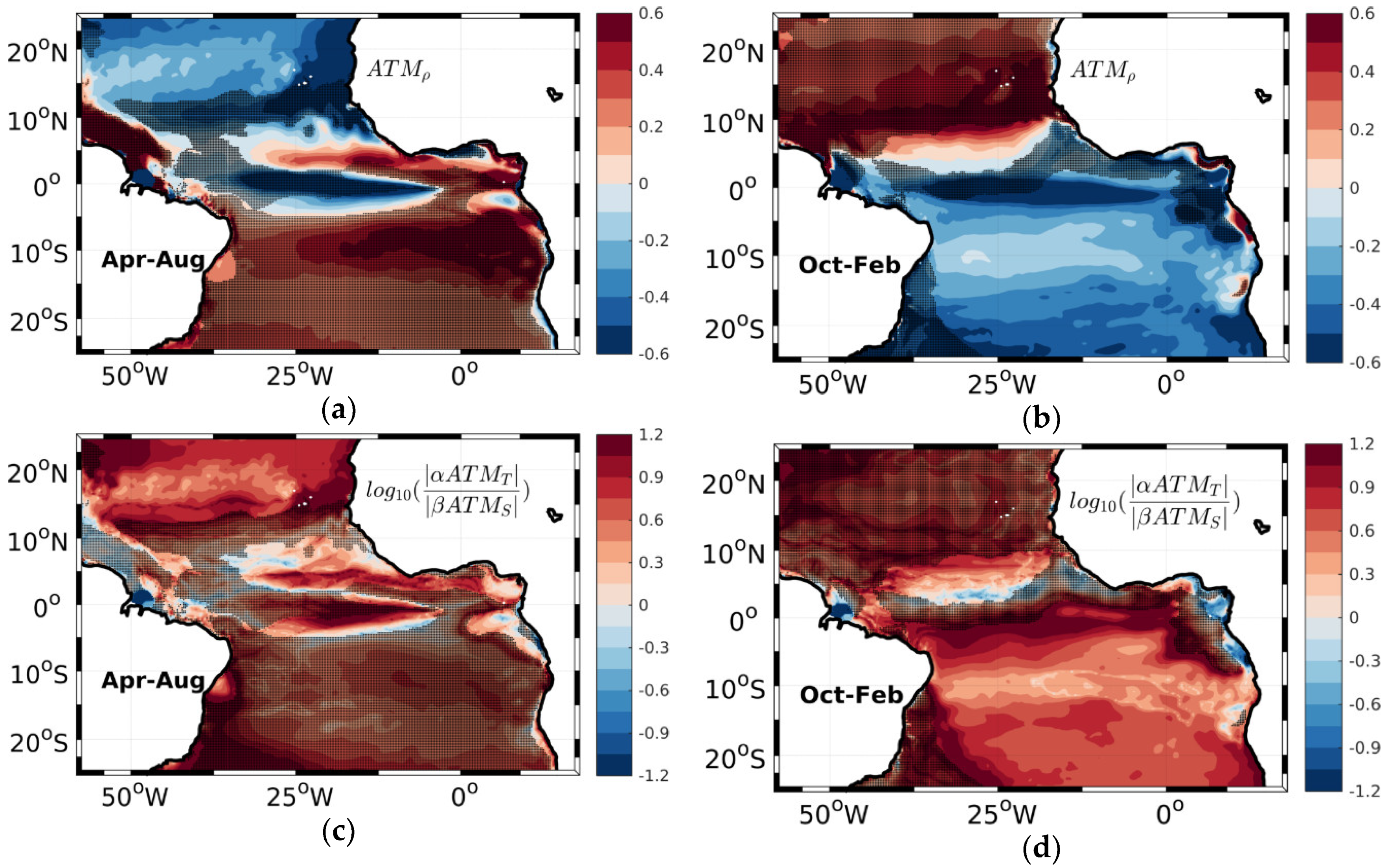
3.1. Atmospheric Physical Processes Contribution
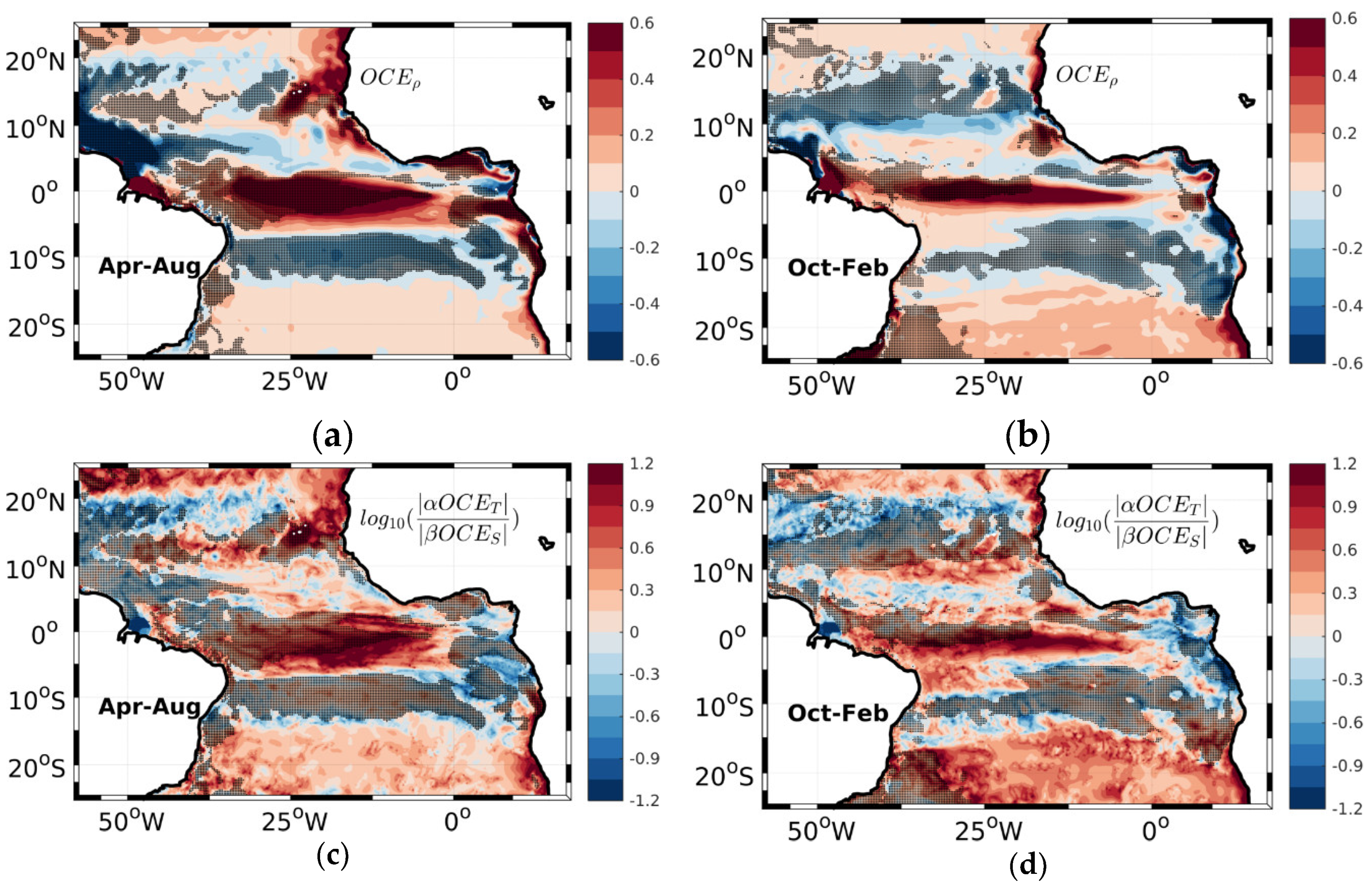
3.2. Oceanic Physical Processes Contribution
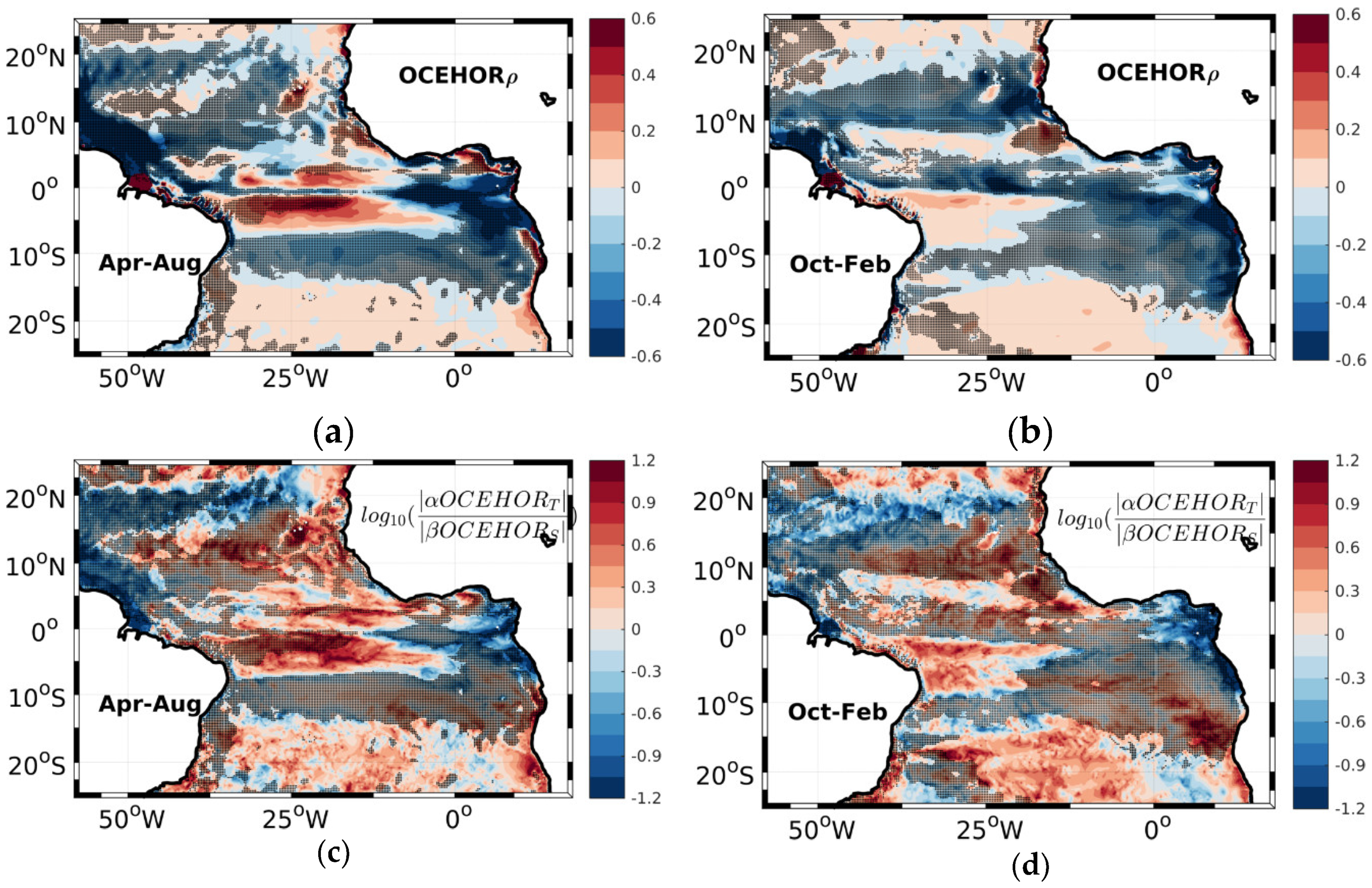
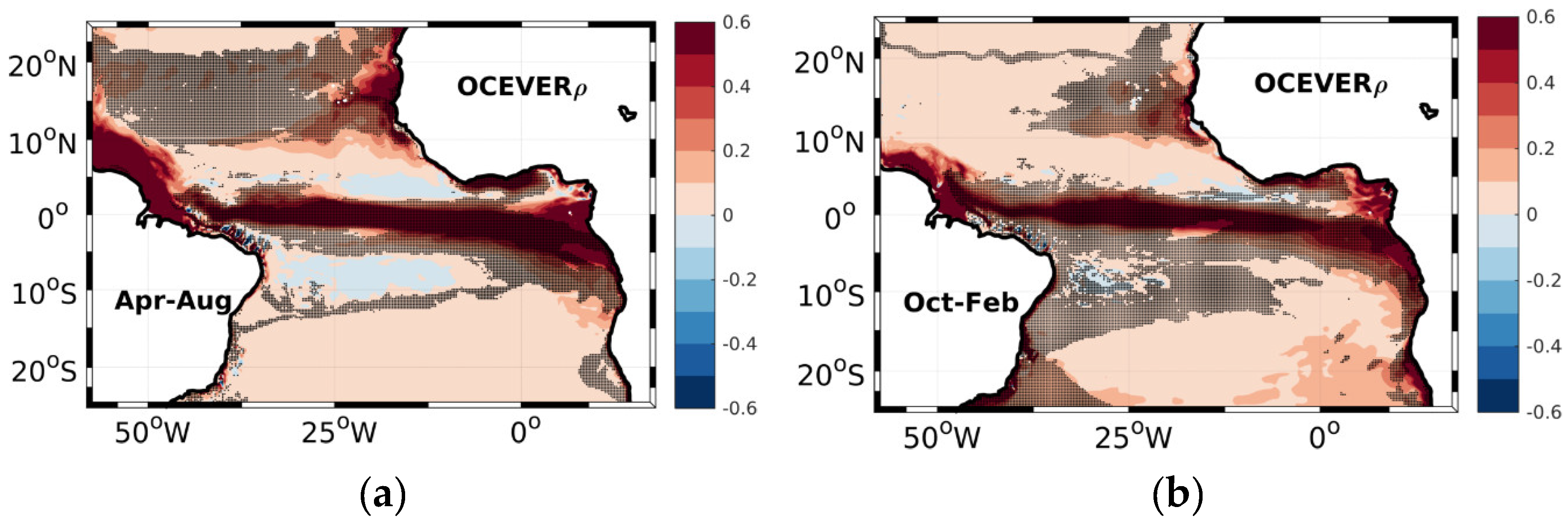
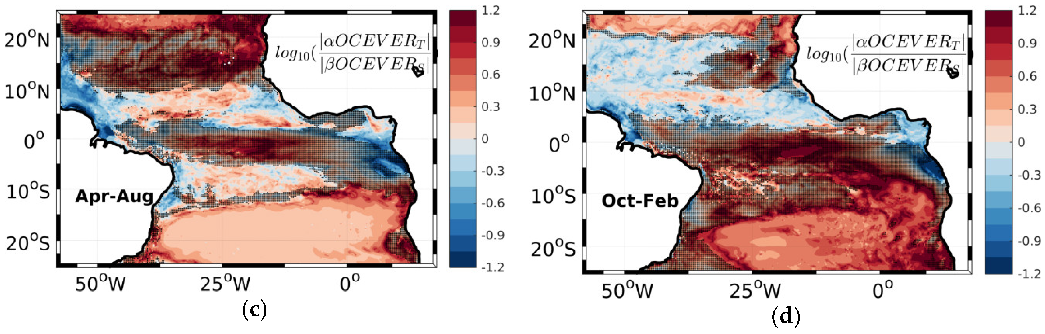
3.3. Horizontal and Vertical Oceanic Physical Processes Contribution
4. Conclusions and Discussion
Author Contributions
Funding
Acknowledgments
Conflicts of Interest
References
- Haine, T.W.N.; Marshall, J. Gravitational, Symmetric, and Baroclinic Instability of the Ocean Mixed Layer. J. Phys. Oceanogr. 1998, 28, 634–658. [Google Scholar] [CrossRef]
- Lukas, R.; Lindstrom, E. The mixed layer of the western equatorial Pacific Ocean. J. Geophys. Res. 1991, 96, 3343. [Google Scholar] [CrossRef]
- Godfrey, J.S.; Lindstrom, E.J. The heat budget of the equatorial western Pacific surface mixed layer. J. Geophys. Res. 1989, 94, 8007. [Google Scholar] [CrossRef]
- Balaguru, K.; Chang, P.; Saravanan, R.; Jang, C.J. The barrier layer of the Atlantic warmpool: Formation mechanism and influence on the mean climate. Tellus A Dyn. Meteorol. Oceanogr. 2012, 64, 18162. [Google Scholar] [CrossRef]
- Kolodziejczyk, N.; Hernandez, O.; Boutin, J.; Reverdin, G. SMOS salinity in the subtropical North Atlantic salinity maximum: 2. Two-dimensional horizontal thermohaline variability. J. Geophys. Res. Ocean. 2015, 120, 972–987. [Google Scholar] [CrossRef]
- Donners, J.; Drijfhout, S.S.; Hazeleger, W. Water Mass Transformation and Subduction in the South Atlantic. J. Phys. Oceanogr. 2005, 35, 1841–1860. [Google Scholar] [CrossRef]
- Blanke, B.; Arhan, M.; Lazar, A.; Prévost, G. A Lagrangian numerical investigation of the origins and fates of the salinity maximum water in the Atlantic. J. Geophys. Res. 2002, 107. [Google Scholar] [CrossRef]
- Kolodziejczyk, N.; Gaillard, F. Observation of spiciness interannual variability in the Pacific pycnocline: Variability of spiciness in pacific. J. Geophys. Res. Ocean. 2012, 117. [Google Scholar] [CrossRef]
- Marshall, D. Subduction of water masses in an eddying ocean. J. Mar. Res. 1997, 55, 201–222. [Google Scholar] [CrossRef]
- Tziperman, E.; Speer, K. A study of water mass transformation in the Mediterranean Sea: Analysis of climatological data and a simple three-box model. Dyn. Atmos. Ocean. 1994, 21, 53–82. [Google Scholar] [CrossRef]
- Karstensen, J.; Quadfasel, D. Formation of Southern Hemisphere Thermocline Waters: Water Mass Conversion and Subduction*. J. Phys. Oceanogr. 2002, 32, 3020–3038. [Google Scholar] [CrossRef]
- Johnson, G.C.; Schmidtko, S.; Lyman, J.M. Relative contributions of temperature and salinity to seasonal mixed layer density changes and horizontal density gradients: Global seasonal mixed layer t and s roles. J. Geophys. Res. Ocean. 2012, 117. [Google Scholar] [CrossRef]
- Yeager, S.G.; Large, W.G. Observational Evidence of Winter Spice Injection. J. Phys. Oceanogr. 2007, 37, 2895–2919. [Google Scholar] [CrossRef]
- Boyer, T.; Levitus, S.; Garcia, H.; Locarnini, R.A.; Stephens, C.; Antonov, J. Objective analyses of annual, seasonal, and monthly temperature and salinity for the World Ocean on a 0.25° grid. Int. J. Climatol. 2005, 25, 931–945. [Google Scholar] [CrossRef]
- Wang, C.; Dong, S.; Munoz, E. Seawater density variations in the North Atlantic and the Atlantic meridional overturning circulation. Clim. Dyn. 2010, 34, 953–968. [Google Scholar] [CrossRef]
- Maes, C.; O’Kane, T.J. Seasonal variations of the upper ocean salinity stratification in the Tropics. J. Geophys. Res. Ocean. 2014, 119, 1706–1722. [Google Scholar] [CrossRef]
- Camara, I.; Kolodziejczyk, N.; Mignot, J.; Lazar, A.; Gaye, A.T. On the seasonal variations of salinity of the tropical A tlantic mixed layer. J. Geophys. Res. Ocean. 2015, 120, 4441–4462. [Google Scholar] [CrossRef]
- Foltz, G.R.; Schmid, C.; Lumpkin, R. Transport of Surface Freshwater from the Equatorial to the Subtropical North Atlantic Ocean. J. Phys. Oceanogr. 2015, 45, 1086–1102. [Google Scholar] [CrossRef]
- Yu, L. A global relationship between the ocean water cycle and near-surface salinity. J. Geophys. Res. 2011, 116. [Google Scholar] [CrossRef]
- Da-Allada, C.Y.; du Penhoat, Y.; Jouanno, J.; Alory, G.; Hounkonnou, N.M. Modeled mixed-layer salinity balance in the Gulf of Guinea: Seasonal and interannual variability. Ocean Dyn. 2014, 64, 1783–1802. [Google Scholar] [CrossRef]
- Nurser, A.J.G.; Marsh, R.; Williams, R.G. Diagnosing Water Mass Formation from Air–Sea Fluxes and Surface Mixing. J. Phys. Oceanogr. 1999, 29, 1468–1487. [Google Scholar] [CrossRef]
- Madec, G. NEMO Ocean Engine; Inst. Pierre Simon Laplace: Paris, France, 2008. [Google Scholar]
- Roullet, G.; Madec, G. Salt conservation, free surface, and varying levels: A new formulation for ocean general circulation models. J. Geophys. Res. Ocean. 2000, 105, 23927–23942. [Google Scholar] [CrossRef]
- Jackett, D.R.; Mcdougall, T.J. Minimal Adjustment of Hydrographic Profiles to Achieve Static Stability. J. Atmos. Ocean. Technol. 1995, 12, 381–389. [Google Scholar] [CrossRef]
- Molines, J.M.; Barnier, B.; Penduff, T.; Brodeau, L.; Treguier, A.M.; Theetten, S.; Treguier, S.; Theetten, G.M. Definition of the Interannual Experiment orca025-g70, 1958–2004; Lab. des Ecoulements Geophys. et Ind.: Grenoble, France, 2007; p. 34. Available online: https://www.drakkar-ocean.eu/publications/reports/orca025-g70.pdf (accessed on 4 June 2020).
- Brodeau, L.; Barnier, B.; Treguier, A.-M.; Penduff, T.; Gulev, S. An ERA40-based atmospheric forcing for global ocean circulation models. Ocean Model. 2010, 31, 88–104. [Google Scholar] [CrossRef]
- Fofonoff, N.P.; Millard, R.C., Jr. Algorithms for the Computation of Fundamental Properties of Seawater; UNESCO: Paris, France, 1983; p. 53. Available online: http://hdl.handle.net/11329/109 (accessed on 4 June 2020).
- Da-Allada, C.Y.; Alory, G.; du Penhoat, Y.; Kestenare, E.; Durand, F.; Hounkonnou, N.M. Seasonal mixed-layer salinity balance in the tropical Atlantic Ocean: Mean state and seasonal cycle. J. Geophys. Res. Ocean. 2013, 118, 332–345. [Google Scholar] [CrossRef]
- Kolodziejczyk, N.; Gaillard, F. Variability of the Heat and Salt Budget in the Subtropical Southeastern Pacific Mixed Layer between 2004 and 2010: Spice Injection Mechanism. J. Phys. Oceanogr. 2013, 43, 1880–1898. [Google Scholar] [CrossRef]
- Wade, M.; Caniaux, G.; du Penhoat, Y. Variability of the mixed layer heat budget in the eastern equatorial Atlantic during 2005–2007 as inferred using Argo floats. J. Geophys. Res. 2011, 116. [Google Scholar] [CrossRef]
- Hasson, A.; Delcroix, T.; Boutin, J.; Dussin, R.; Ballabrera-Poy, J. Analyzing the 2010-2011 La Niña signature in the tropical Pacific sea surface salinity using in situ data, SMOS observations, and a numerical simulation. J. Geophys. Res. Ocean. 2014, 119, 3855–3867. [Google Scholar] [CrossRef]
- Peter, A.-C.; Le Hénaff, M.; du Penhoat, Y.; Menkes, C.E.; Marin, F.; Vialard, J.; Caniaux, G.; Lazar, A. A model study of the seasonal mixed layer heat budget in the equatorial Atlantic. J. Geophys. Res. 2006, 111. [Google Scholar] [CrossRef]
- Vialard, J.; Foltz, G.R.; McPhaden, M.J.; Duvel, J.P.; de Boyer Montégut, C. Strong Indian Ocean sea surface temperature signals associated with the Madden-Julian Oscillation in late 2007 and early 2008. Geophys. Res. Lett. 2008, 35. [Google Scholar] [CrossRef]
- Gentemann, C.L.; Wentz, F.J.; Brewer, M.; Hilburn, K.; Smith, D. Passive Microwave Remote Sensing of the Ocean: An Overview. In Oceanography from Space; Barale, V., Gower, J.F.R., Alberotanza, L., Eds.; Springer: Dordrecht, The Netherlands, 2010; pp. 13–33. [Google Scholar] [CrossRef]
- Reynolds, R.W.; Smith, T.M. A High-Resolution Global Sea Surface Temperature Climatology. J. Clim. 1995, 8, 1571–1583. [Google Scholar] [CrossRef]
- Boutin, J.; Vergely, J.L.; Marchand, S.; D’Amico, F.; Hasson, A.; Kolodziejczyk, N.; Reul, N.; Reverdin, G.; Vialard, J. New SMOS Sea Surface Salinity with reduced systematic errors and improved variability. Remote Sens. Environ. 2018, 214, 115–134. [Google Scholar] [CrossRef]
- Kolodziejczyk, N.; Boutin, J.; Vergely, J.-L.; Marchand, S.; Martin, N.; Reverdin, G. Mitigation of systematic errors in SMOS sea surface salinity. Remote Sens. Environ. 2016, 180, 164–177. [Google Scholar] [CrossRef]
- Jin, J.-B.; Zeng, Q.-C.; Liu, H.-L.; Wu, L. The impacts of different surface boundary conditions for sea surface salinity on simulation in an OGCM. Atmos. Ocean. Sci. Lett. 2016, 9, 465–470. [Google Scholar] [CrossRef]
- Large, W.G.; Danabasoglu, G.; Doney, S.C.; McWilliams, J.C. Sensitivity to Surface Forcing and Boundary Layer Mixing in a Global Ocean Model: Annual-Mean Climatology. J. Phys. Oceanogr. 1997, 27, 2418–2447. [Google Scholar] [CrossRef]
- Servain, J.; Lazar, A. Ocean Dynamics Contribution to Seasonal Mixed Layer Heat Budget in the Tropical Atlantic. In Clima do Atlântico Tropical e Impactos Sobre o Nordeste (CATIN); FUNCEME: Fortaleza, Brazil; IRD: Wellington, New Zealand, 2010; p. 392, (Serie Oceanografia e Meteorologia da Funceme; 1); ISBN 978-85-62406-07-2. [Google Scholar]
- Faye, S.; Lazar, A.; Sow, B.A.; Gaye, A.T. A model study of the seasonality of sea surface temperature and circulation in the Atlantic North-eastern Tropical Upwelling System. Front. Phys. 2015, 3. [Google Scholar] [CrossRef]
- Jouanno, J.; Marin, F.; du Penhoat, Y.; Sheinbaum, J.; Molines, J.-M. Seasonal heat balance in the upper 100 m of the equatorial Atlantic Ocean. J. Geophys. Res. 2011, 116. [Google Scholar] [CrossRef]
- Foltz, G.R.; McPhaden, M.J. Seasonal mixed layer salinity balance of the tropical North Atlantic Ocean. J. Geophys. Res. 2008, 113. [Google Scholar] [CrossRef]
- Mignot, J.; de Boyer Montégut, C.; Lazar, A.; Cravatte, S. Control of salinity on the mixed layer depth in the world ocean: 2. Tropical areas. J. Geophys. Res. 2007, 112. [Google Scholar] [CrossRef]
- Griffies, S.M.; Biastoch, A.; Böning, C.; Bryan, F.; Danabasoglu, G.; Chassignet, E.P.; England, M.H.; Gerdes, R.; Haak, H.; Hallberg, R.W.; et al. Coordinated Ocean-ice Reference Experiments (COREs). Ocean Model. 2009, 26, 1–46. [Google Scholar] [CrossRef]
- Behrens, E.; Biastoch, A.; Böning, C.W. Spurious AMOC trends in global ocean sea-ice models related to subarctic freshwater forcing. Ocean Model. 2013, 69, 39–49. [Google Scholar] [CrossRef]
- Danabasoglu, G.; Yeager, S.G.; Bailey, D.; Behrens, E.; Bentsen, M.; Bi, D.; Biastoch, A.; Boning, C.; Bozec, A.; Canuto, V.M.; et al. North Atlantic simulations in Coordinated Ocean-ice Reference Experiments phase II (CORE-II). Part I: Mean states. Ocean Model. 2014, 73, 76–107. [Google Scholar] [CrossRef]
- Delcroix, T.; Chaigneau, A.; Soviadan, D.; Boutin, J.; Pegliasco, C. Eddy-induced salinity changes in the tropical Pacific. J. Geophys. Res. Ocean. 2019, 124, 374–389. [Google Scholar] [CrossRef]
- Stewart, K.D.; Haine Thomas, W.N.; McC. Hogg, A.; Roquet, F. On cabbeling and thermobaricity in the surface mixed layer. J. Phys. Oceanogr. 2017, 47, 1775–1787. [Google Scholar] [CrossRef]


© 2020 by the authors. Licensee MDPI, Basel, Switzerland. This article is an open access article distributed under the terms and conditions of the Creative Commons Attribution (CC BY) license (http://creativecommons.org/licenses/by/4.0/).
Share and Cite
Camara, I.; Mignot, J.; Kolodziejczyk, N.; Losada, T.; Lazar, A. Tropical Atlantic Mixed Layer Buoyancy Seasonality: Atmospheric and Oceanic Physical Processes Contributions. Atmosphere 2020, 11, 649. https://doi.org/10.3390/atmos11060649
Camara I, Mignot J, Kolodziejczyk N, Losada T, Lazar A. Tropical Atlantic Mixed Layer Buoyancy Seasonality: Atmospheric and Oceanic Physical Processes Contributions. Atmosphere. 2020; 11(6):649. https://doi.org/10.3390/atmos11060649
Chicago/Turabian StyleCamara, Ibrahima, Juliette Mignot, Nicolas Kolodziejczyk, Teresa Losada, and Alban Lazar. 2020. "Tropical Atlantic Mixed Layer Buoyancy Seasonality: Atmospheric and Oceanic Physical Processes Contributions" Atmosphere 11, no. 6: 649. https://doi.org/10.3390/atmos11060649
APA StyleCamara, I., Mignot, J., Kolodziejczyk, N., Losada, T., & Lazar, A. (2020). Tropical Atlantic Mixed Layer Buoyancy Seasonality: Atmospheric and Oceanic Physical Processes Contributions. Atmosphere, 11(6), 649. https://doi.org/10.3390/atmos11060649