Article

The Use of a Numerical Weather Prediction Model to Simulate Near-Field Volcanic Plumes

1
National Centre for Atmospheric Science, Fairbairn House, Leeds LS2 9PH, UK
2
School of Earth Sciences and School of Mathematics, University of Bristol, Bristol BS8 1TH, UK
*
Author to whom correspondence should be addressed.
Atmosphere 2020, 11(6), 594; https://doi.org/10.3390/atmos11060594
Submission received: 16 April 2020 / Revised: 13 May 2020 / Accepted: 27 May 2020 / Published: 4 June 2020
(This article belongs to the Special Issue Forecasting the Transport of Volcanic Ash in the Atmosphere)

Abstract

:
In this paper, a state-of the art numerical weather prediction (NWP) model is used to simulate the near-field plume of a Plinian-type volcanic eruption. The NWP model is run at very high resolution (of the order of 100 m) and includes a representation of physical processes, including turbulence and buoyancy, that are essential components of eruption column dynamics. Results are shown that illustrate buoyant gas plume dynamics in an atmosphere at rest and in an atmosphere with background wind, and we show that these results agree well with those from theoretical models in the quiescent atmosphere. For wind-blown plumes, we show that features observed in experimental and natural settings are reproduced in our model. However, when comparing with predictions from an integral model using existing entrainment closures there are marked differences. We speculate that these are signatures of a difference in turbulent mixing for uniform and shear flow profiles in a stratified atmosphere. A more complex implementation is given to show that the model may also be used to examine the dispersion of heavy volcanic gases such as sulphur dioxide. Starting from the standard version of the weather research and forecasting (WRF) model, we show that minimal modifications are needed in order to model volcanic plumes. This suggests that the modified NWP model can be used in the forecasting of plume evolution during future volcanic events, in addition to providing a virtual laboratory for the testing of hypotheses regarding plume behaviour.

1. Introduction

Forecasting the dispersion of volcanic ash and gases produced during volcanic eruptions is crucial for the management of hazards during volcanic eruptions. Numerous atmospheric dispersion models (e.g., NAME [1], FALL3D [2], Ash3d [3]) are in use (in both research and operational capacities) that forecast the far-field transport of volcanic ash in the atmosphere. However, accurate forecasts rely on the imposition of boundary conditions that model the transport of volcanic eruption products from the volcanic vent into the atmosphere in the eruption column. The eruption column is a multiphase, turbulent buoyant jet with complicated dynamics that are not included in far-field dispersion models. Therefore, far-field dispersion models require a representation of the eruption column as a boundary condition. Of particular importance is the rate at which ash and gases are erupted from the volcano (referred to as the source mass flux or the mass eruption rate) and the height at which this material is injected into the atmosphere. Together, these two values are often referred to as the ‘source term’, and they are related by the dynamics of the eruption column proximal to the vent.
Sophisticated models of eruption column dynamics have been developed, using advanced computational fluid dynamics (CFD) methodologies [4,5,6,7] that simulate turbulent, multiphase flows. A variety of physical processes have been included in these models, including particle fallout, particle aggregation, phase change of entrained water vapour, and cloud microphysics [8]. Such CFD models allow the effects of these interacting processes to be assessed, but are computationally demanding, limiting their use in operational settings. Furthermore, the meteorological controls on plume dynamics are not fully integrated.
The complicated dynamics of the eruption column has led to simplified descriptions to estimate the source term. For example, dispersion models such as the UK Met Office NAME model [1] often use calibrated algebraic relationships between the source mass flux and the plume height [9,10] to estimate the source term for explosive eruptions that produce buoyant eruption columns. These relationships are based upon a data set of historical eruptions, and relate the mass flux to the observed plume height, and thus allow a mass flux to be inferred from an observation of plume height (the latter being routine to estimate in situ, the former extremely difficult). We subsequently refer to these relationships as the Sparks-Mastin curves, sometimes known as the empirical Mastin relationship. Importantly, the Sparks-Mastin curves do not discriminate between regimes of differing background wind speed or atmospheric stratification (or rather, they contain this information only implicitly, and variations are aggregated into the calibrated curve fit). Recent work [11,12,13] has sought to enhance the functionality of these empirical relationships by modelling the effect of wind on the eruption column dynamics, based on a re-analysis of historical data with appropriate background wind speed determined from meteorological reanalyses) and theoretical models of wind-blown buoyant plumes [14]. This type of approach cannot, by their very nature, allow sophisticated representations of atmospheric processes and features such as three-dimensional turbulence, microphysics, radiation and temperature inversions (and the interactions between these), but must include their effects via simplified parametrisations or calibration using field observations.
An alternative approach has been to develop simplified mathematical descriptions of turbulent plumes [15] and volcanic eruption columns [9,16,17]. These models (often referred to as plume-rise models) average over the turbulent time scale and integrate over a cross section of the plume (and are therefore known as ‘integral’ models), resulting in a system of ordinary differential equations (in the steady case) that can be solved efficiently using standard computational methods. The influence of atmospheric conditions (including non-uniform stratification and wind) on the plume dynamics has been incorporated into these integral model, allowing their effects to be explored (e.g., [9,12,16]), and their rapid implementation allows inverse calculations to be performed to estimate the source conditions from plume height observations [12,18]. However, in deriving the simplified description, a parameterization of some physical processes, notably turbulent mixing, is required and the model predictions are strongly dependent on the calibration of these parameterisations [18]. Furthermore, the coupling of the plume dynamics to the local atmospheric structure is not fully modelled; there is only a one-way coupling, with atmospheric structure influencing plume dynamics, but no feedback from the plume dynamics onto the local atmosphere.
Numerical weather prediction (NWP) models may present an approach to overcome the limitations of CFD and integral plume models and semi-empirical relationships, allowing plume dynamics, ash dispersion and meteorology to be simulated within a single numerical package. The use of NWP models in volcanic ash dispersal modelling is usually implemented at large spatial scales, commonly by driving an advection-diffusion model with meteorological fields, typically by artificially introducing volcanic ash particles [19,20], allowing an examination of, e.g., orographic flow effects [21,22]. In this study, we use an NWP model at very high resolution to simulate the near-field plume behaviour, and the plume is simulated in the body of the NWP code.
The near-field of a volcanic plume is of significance since this is the region where pollutant is particularly susceptible to atmospheric turbulence, thermal stratification, etc. which influence the height and layering of the plume (with significant consequences for the long range dispersion), and the plume dynamics can feedback onto the atmospheric structure. The use of an NWP model allows complex meteorological and dynamical processes to be included in the development of the modelling framework. This paper is concerned with near-field plume dynamics, but the use of an NWP model additionally allows the dispersal of pollutant over extended temporal and spatial scales to be investigated, with the potential of incorporation into routine operational meteorological forecasts. Furthermore, NWP models are subject to continuous revision and improvement to their parametrisations and representations of physical effects, and so should represent the state-of-the-art in both numerical methods and physical understanding of atmospheric processes. Thus, the ability to incorporate a near-field plume package into an NWP model would be of great benefit. In this paper the ability of an NWP model to simulate the behaviour of a buoyant gas plume is demonstrated. Further work and subsequent studies will allow a more elaborate implementation, incorporating aspects of physical ash dispersal. This paper is designed as a proof-of-concept study. However, a relatively simple additional change allows the model to simulate the release of a dense gas.
The purpose of this paper is to describe the NWP plume model setup and to present a number of examples of its application aimed principally at demonstrating the utility, accuracy and scope of this novel approach to volcanic plume modelling. In Section 2, the NWP model to be used is introduced. Section 3 discusses some results from the model, with further, more complex examples of its use given in Section 4. The work is summarised in Section 5.

2. Numerical Experiments

2.1. The Use of the Weather Research and Forecasting Model

A number of numerical models, of varying degrees of complexity and sophistication, have been used in the past to study and simulate volcanic plumes [4,7,8,23,24,25]. Such models typically have a sophisticated representation of the source term but do not have the full suite of physical parametrisations that a numerical weather prediction model (NWP) has. Some models have an online chemical transport component (e.g., [19,26]) but such models are often very expensive to run (and are run usually at low resolutions, i.e., large grid sizes). For example, the Weather Research and Forecasting Chemistry model WRF-CHEM [27] model has been used to treat the dispersal of ash [28]. WRF-CHEM is very computationally expensive to use at the high resolutions used in this paper (typically, WRF-CHEM requires between a factor of 2 and 100 greater time to compute than the corresponding WRF run [29]), and would normally be used to study the long-range/low-resolution transport of volcanic material. WRF-CHEM does include a volcano model, however the source-term is represented using the Sparks-Mastin curves. Since we wish to determine an alternative to the use of such curves, the use of WRF-CHEM was avoided.
Instead, we have taken a widely available NWP model (the Weather Research and Forecasting model [30]; WRF) and introduced relatively small changes to the code, that allow the base model to be used in dispersion studies. The WRF model has been used widely in meteorological modelling, both operationally and as a method of analysing individual test cases. Free to use, it has over 48,000 registered users in 160 countries [31]. It has been used operationally by Meteorological Agencies in over 50 countries, covering North and South America, Europe, Scandinavia, Africa, the Middle East, and Asia, including Russia and China [32].
WRF is a state-of-the-art numerical weather prediction program, developed at the National Center for Atmospheric Research (NCAR) and other US agencies and institutes, and it is relatively easy to learn to use and to implement. WRF is non-hydrostatic, compressible, and fully three-dimensional. It has a full range of physical parametrisations, including representations of the boundary-layer, clouds, microphysics, radiation and turbulence. In addition, a land-surface model that includes vegetative and evapotranspiration effects is included. The model is capable of being operated in a mode akin to large-eddy-simulations, with the boundary layer parametrisation switched off; the largest eddies are thus those explicitly represented in the model, with turbulence on the sub-grid scale being parametrised. See Appendix A for a summary of the governing equations used in WRF (including a summary of the turbulence closure scheme) and see Appendix B for the model-specific choices made in this study.
WRF incorporates the very latest developments in its physical parametrisations and numerical methods and has a major new release typically every six months. The model can be implemented at a variety of spatial scales, from hundreds of metres to tens of kilometres [33]. The computational implementation is fully parallel and so the scale of run is limited only by the computational resources available. In the following, the version of WRF used is WRF 3.5.1, but it should be emphasised that the methodology is not particular to this version, and applies to all successive and future versions of the model (provided the backward-compatibility of WRF updates is maintained).
The advantages of using WRF as a “host” for a plume and dispersion model are that the atmospheric fluid dynamics solver routines are well tested, there is a worldwide user community (including operational use) together with the support network that such widespread use encourages, and active development and testing (through peer review). The range of grid resolutions (from tens of metres to tens of kilometres) that WRF can be initiated on makes it ideal as a testbed for dispersion studies. The model can be run on relatively low numbers of processors; the results in this paper were obtained on an inexpensive multi-processor machine. The results presented here took of the order of several hours using 24 processors. However, the ability to use hundreds of processors means that the same results can be obtained very quickly if desired, making this approach viable for disaster mitigation and operational use. The model can also be run in a nested mode, whereby domains are nested within “parent” domains of lower resolution, providing locally high spatial resolution in regions where small scales are strongly influencing the dynamics without committing computational resources where they are not required. Thus, there is considerable benefit in using such a model to simulate the behaviour of volcanic plumes.
The framework implemented here represents a buoyant plume model, and does not include particulates explicitly. A version of the model (simulating dense gas, see Section 4) has demonstrated that the model can capture the observed dispersion associated with regions of complex topography: such complex flows are not captured by models that do not include topography, or that only include it at coarse resolutions. Additionally, the authors plan (in future work) to add momentum equations for the ash phase itself to the WRF equation set, and thus turn WRF into a full multiphase model.

2.2. Initialisation Method

WRF is capable of being initialised from host-model analyses, e.g., the National Centre for Environmental Prediction’s Global Forecast System [34] model data. These data then forms the boundary conditions for the model, the boundaries being updated at every model time-step (based upon an interpolation of the T-hourly analysis/forecast data). Alternatively, it can (when run in ‘idealised’ mode) be initialised via a single vertical profile of wind, temperature and moisture, corresponding to a case of interest. In this case, the boundary conditions can be open, periodic, or symmetric, while open boundaries are implemented in the following cases.
At the upper boundary, a sponge layer is used to gradually diminish signals/waves that are propagating out of the computational domain while minimizing spurious reflections. While these boundary conditions are designed to allow information to propagate out of the computational domain, it is possible that numerical artefacts due to imprecise boundary conditions can affect the calculated solution. Therefore, in the tests that follow, the positions of the lateral and upper boundaries are chosen so that any boundary-condition artefacts are far from the source region. The lower boundary models the topography of the ground. In Section 3, the surface is taken to be flat, while in Section 4 we introduce topography to illustrate the ability to model orographic flows.
To model the volcanic source, a large thermal perturbation is imposed at the surface, at the location of the vent. A thermal perturbation has previously been used in WRF to model convection and precipitation over a volcanic landscape during dome-building (where a hot lava dome is extruded on the volcano) [35], however, for explosive eruptions, the thermal perturbation is substantially larger. The vent is taken to be circular with a radius of 200 m (the model regular grid spacing means the vent is never exactly circular, however) at ground level and horizontally centred in the domain. A passive tracer is released at a constant rate and is co-located with the thermal perturbation. The actual thermal perturbation determines the plume rise height in this case (as will be discussed later). These thermal perturbations produce large upwardly directed vertical velocities, on the order of 50 ms−1. These locally large flow speeds result in small time steps since WRF is an Eulerian model and thus the time-step is severely restricted by the Courant–Friedrichs–Lewy (CFL) condition (see, e.g., [36]).
In the following results, the maximum acceptable time step was found to be 0.25 s. Note that acoustic modes are dealt with separately by the model dynamics and have an associated time step of, typically, 0.025 s. In this framework the severe updraughts representing the volcanic eruption are notionally equivalent to those of a very severe thunderstorm (albeit one which has a continuous forcing mechanism). It is possible (and quite straight-forward) to implement an additional “jet” of fluid from the source to model the momentum-driven ejection of material at the volcanic vent. However, here we do not model the near-vent jet, i.e., all updraughts arise from buoyancy.
The model domain is configured to be 30 × 30 km in the horizontal, with a resolution of 100 m. The vertical resolution is variable: there are 141 vertical levels (seven levels in the lowest 1000 m) with the model top at 30 hPa. This configuration prevents the gravity waves generated in the model and their subsequent reflections at model boundaries from interfering with the region of interest. The surface thermal perturbation is here taken to be constant in time, although it is trivial to introduce time variation in the source to model unsteady eruptions. The model results presented in Section 3 are effectively one-way coupled: atmospheric motion affects the tracer, but not vice-versa. In a real eruption this is not strictly the case, and the ash particles can themselves generate turbulence and affect the motion of surrounding air (see, e.g., [37]). To include two-way coupling with ash—in other words, to allow the model to be run in full multiphase mode—is an ongoing subject of study. However, a two-way coupling is possible if the ejected matter is considered as a dense gas (such as sulphur dioxide), and in Section 4 results illustrating the dynamics in this regime are presented
In this study, the microphysics, radiation and land-surface schemes are switched off, to enable comparison with theoretical models that do not include the effects of these physical processes. Such physical schemes can be run concurrently with the plume simulations, but our aim is to compare the results with standard theoretical approaches, and no such simple theoretical approaches currently exist to deal with the effect of (for example) short-wave radiation upon plume height. The present paper is not intended to be an exhaustive treatment of, nor a study of the sensitivities to, these physical processes, but is rather intended to demonstrate the feasibility of conducting such tests in the future. As such the modelling work presented here represents a framework upon which further studies can be incorporated.
All simulations are conducted in large-eddy simulation mode, where the boundary-layer parametrisation is switched off and the larger eddies (of the order of 100 m) are explicitly resolved. Smaller eddies are resolved via a turbulence-kinetic-energy (TKE)-based sub-grid turbulence scheme, acting on full (not perturbation) fields; second-order horizontal diffusion acts on model surfaces. A brief description of the turbulence scheme is given in Appendix A. For a full description of the WRF TKE scheme, see [30]. No initial (or background, or ambient) turbulence is included in the model, for the reason of simplicity. Subsequent studies could examine the role of background turbulence or turbulence near the source. This could then allow further study of the role of entrainment (as in [38]), but this is beyond the scope and purpose of this paper.
We emphasise that no additional equations of motion were added to the model. The governing model equations are the flux-form Euler equations (conservative for scalar variables), treated via a terrain-following hydrostatic-pressure vertical coordinate. The grid is of Arakawa-C type [39], with integration performed by a time-split Runge-Kutta scheme. Prognostic variables consist of the three velocity components and perturbations of potential temperature, geopotential, and surface pressure (in addition to a range of physical properties, such as mixing ratios, if these are required). The turbulence is represented by a second-order horizontal diffusion scheme, with no boundary-layer parametrisation. Here, the horizontal diffusion acts on the horizontal gradients, with a vertical correction term. The vertical diffusion acts on the full (rather than perturbation) fields (the recommended approach in WRF). In the implementation below, the heat flux (corresponding to that of the vent) is supplied by the user, with drag terms coming from the model physics. The surface layer is aligned with Monin–Obukhov similarity theory. For a full description of the WRF model equation set, see [30], and for further information on the physical schemes available to the user, see the ARW User Guide [40].
Unless otherwise stated, the thermal stratification is taken to be that of the dry standard U.S. atmosphere [41] at rest. The method is applicable to other stratifications, of course. In Section 4 the effect of altering the background winds is investigated. In the majority of idealised test cases presented here, the surface is taken to be flat; the exception being a demonstration of the method to simulate the spread of dense gas that is erupted from a fissure in Iceland, presented in Section 4, where the surface characteristics (topography, roughness length, etc.) are explicitly included in the model.

3. Results

Here we present the results of WRF simulations of buoyant volcanic plumes rising through quiescent and windy environments. We analyse these results by considering both bulk properties (such as plume rise height scaling) and intrinsic variables.

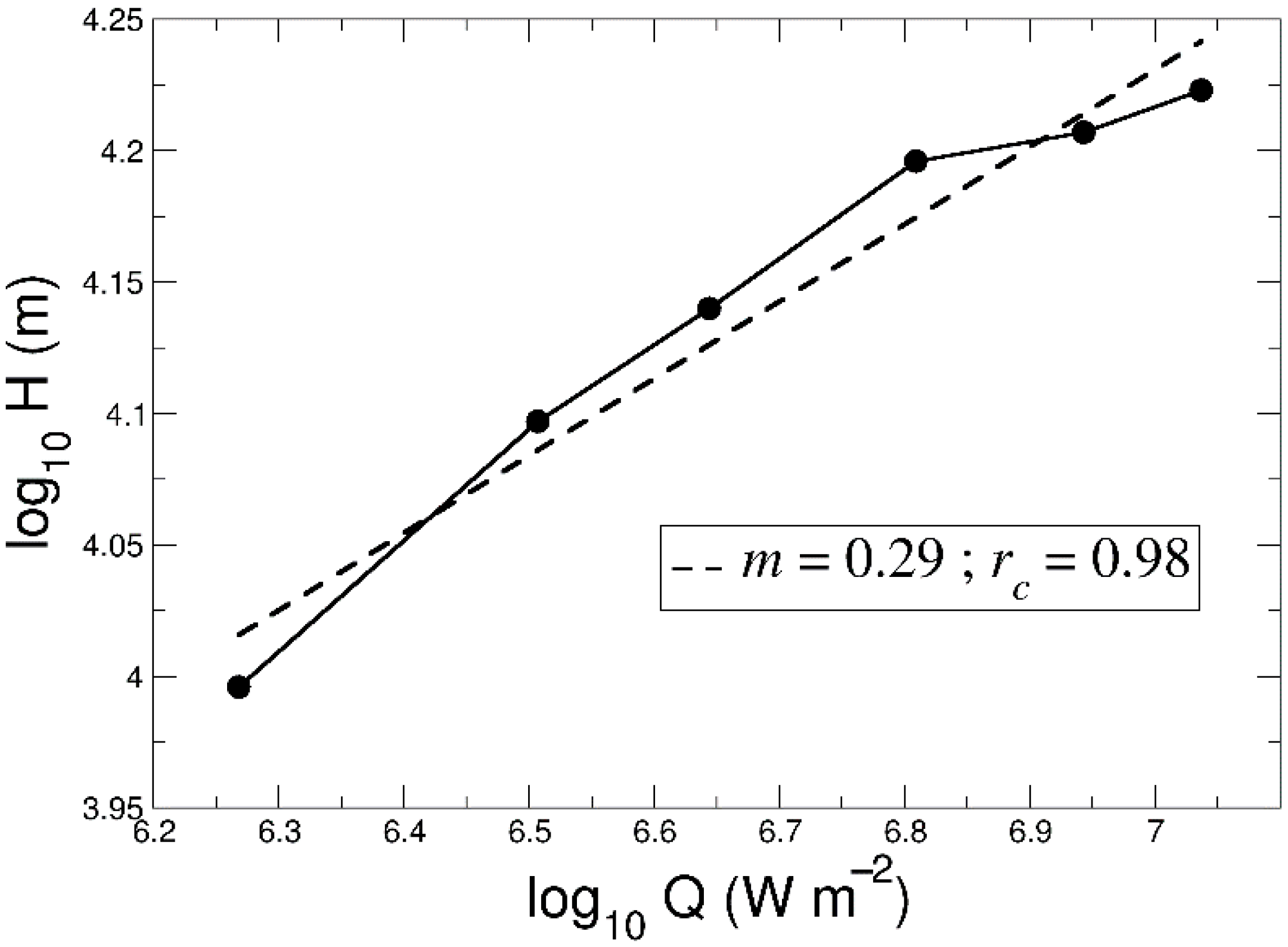
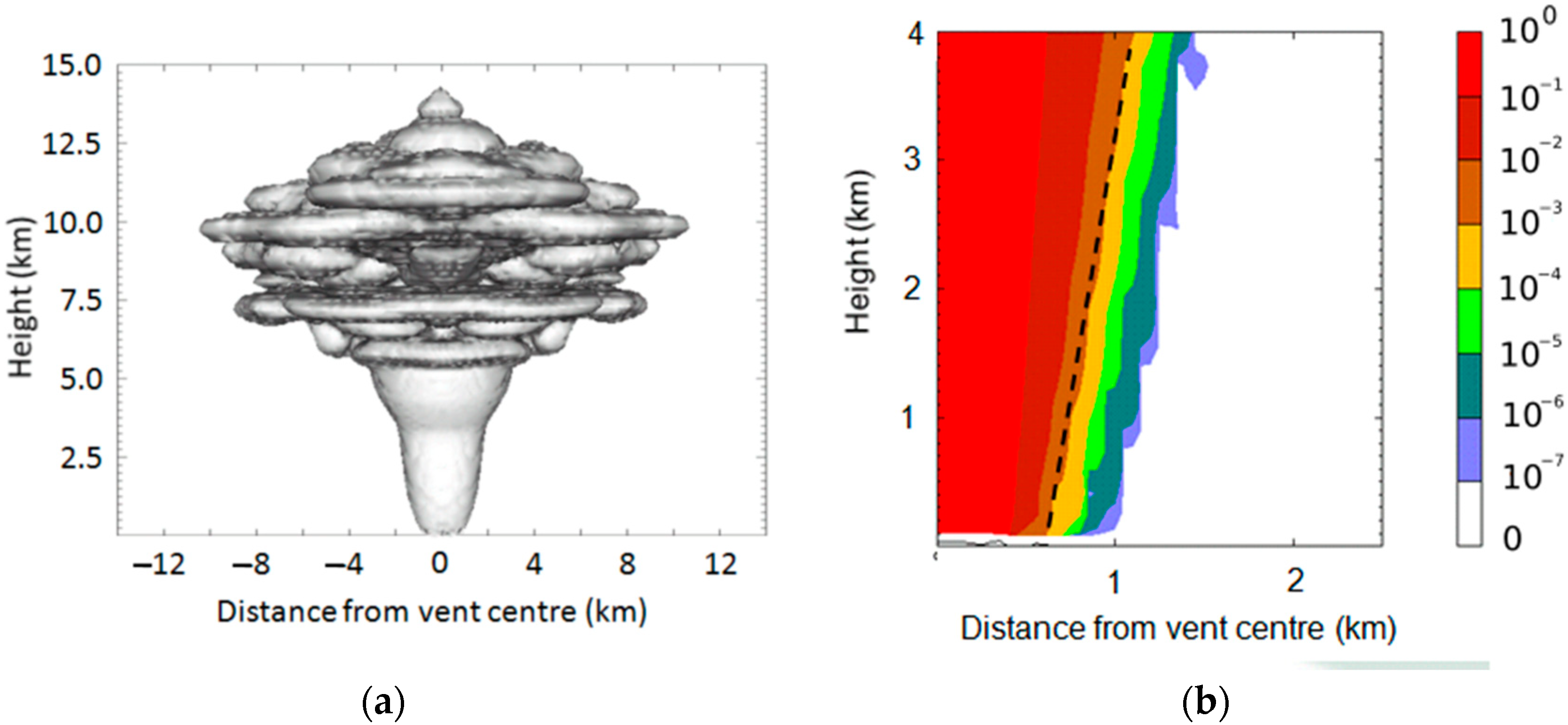
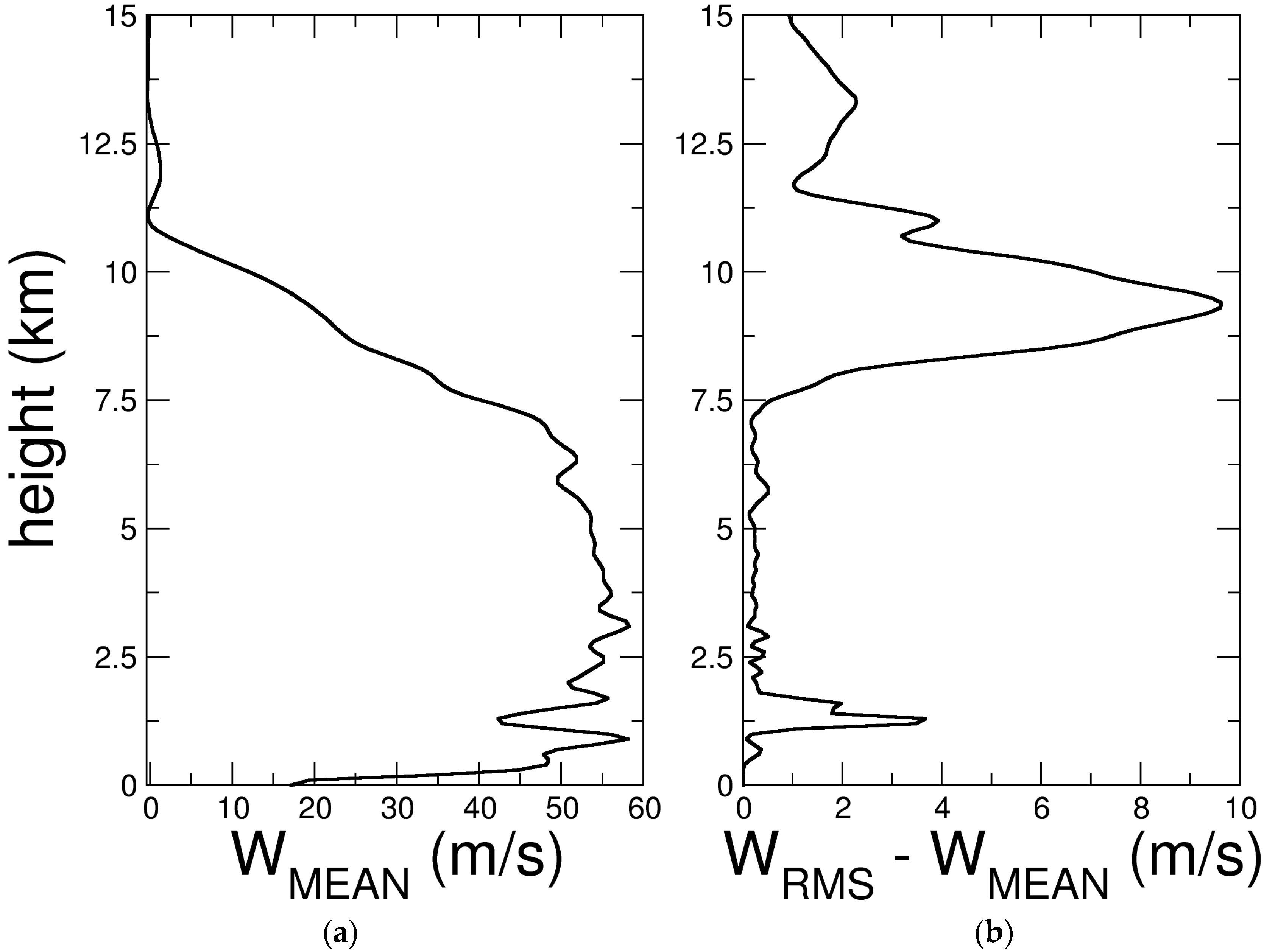
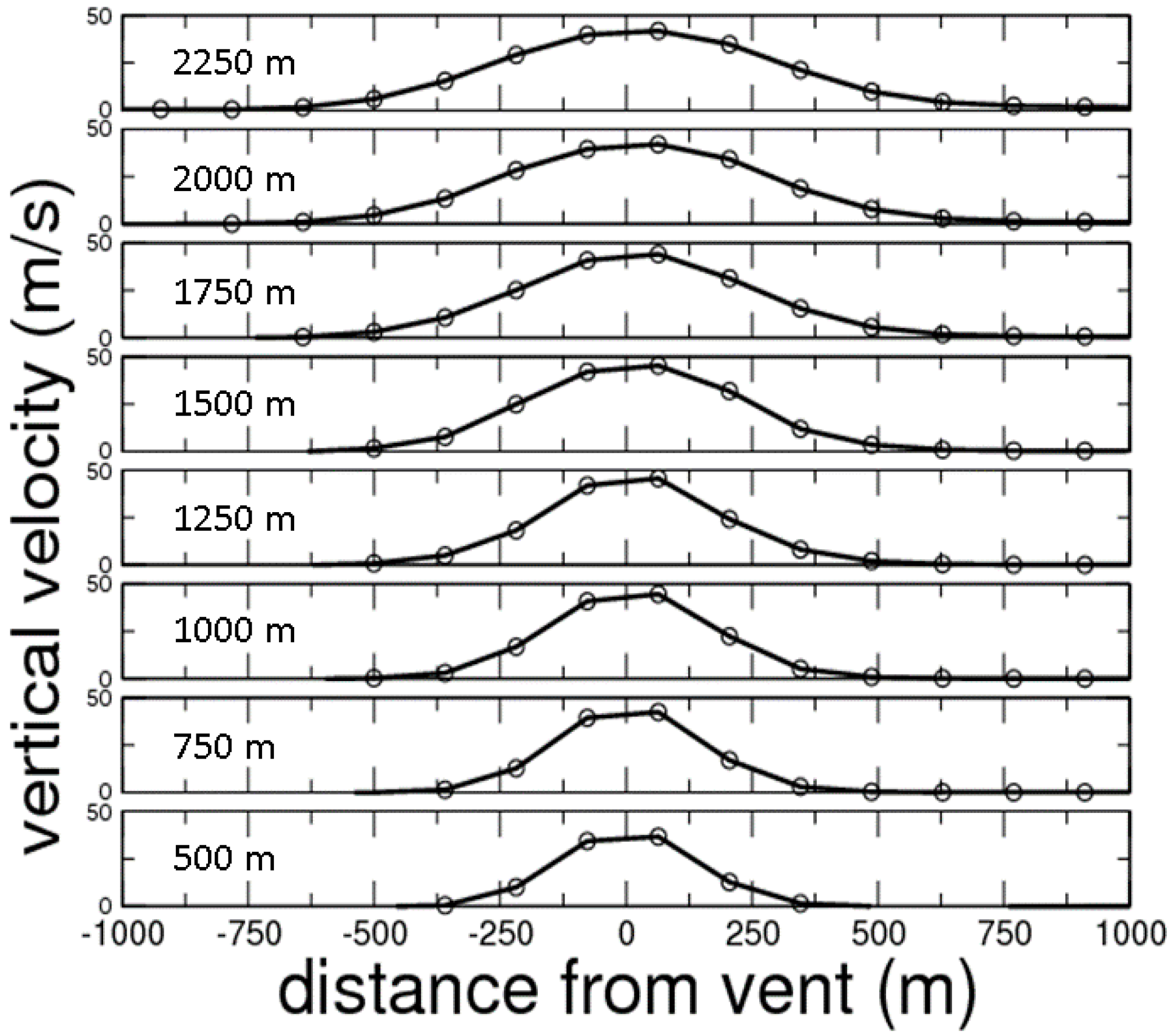
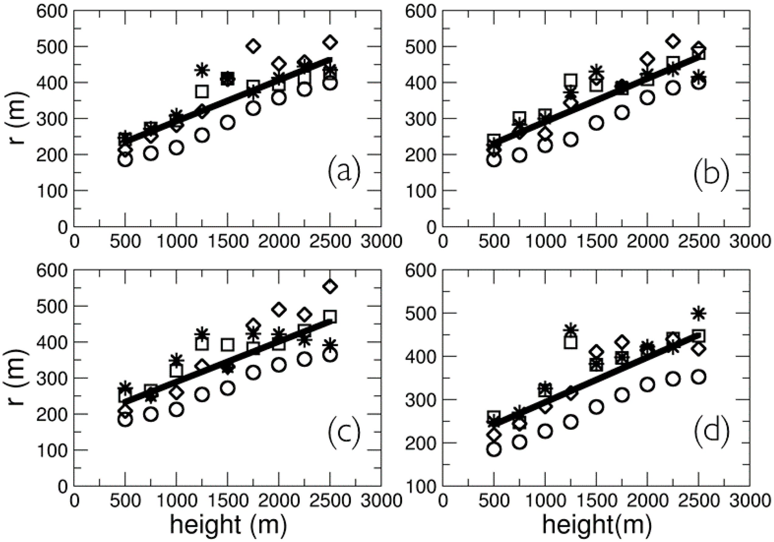
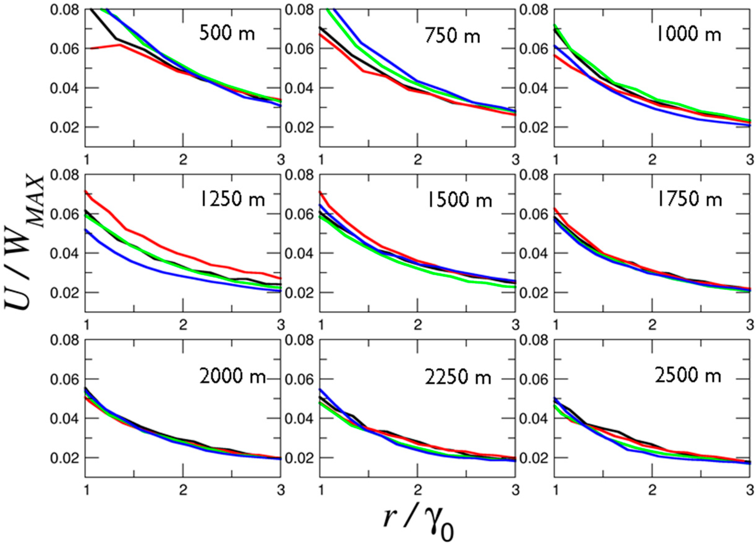
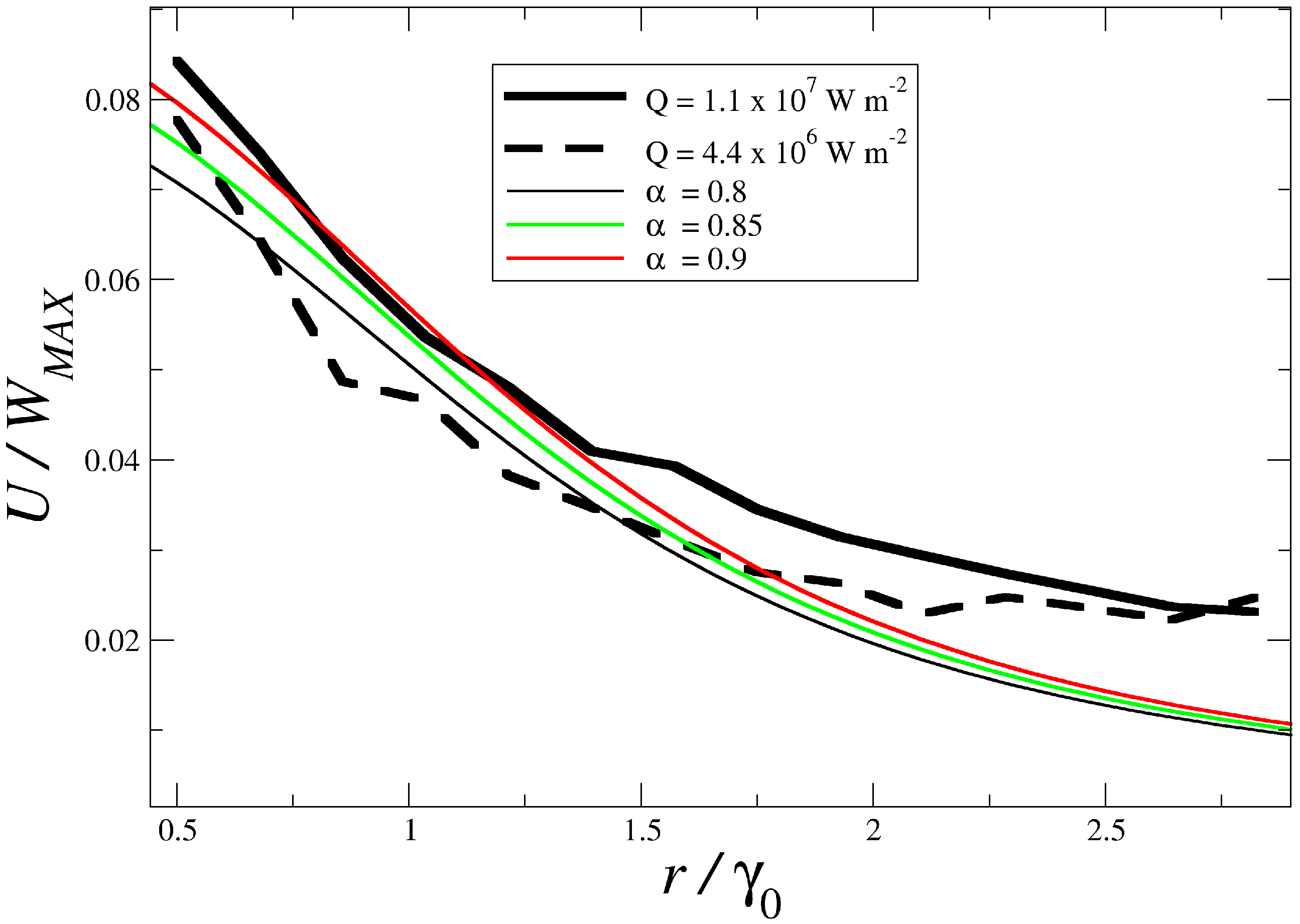
3.1. Plume Characteristics in a Quiescent Atmosphere

A relationship of fundamental importance is that of the rise height of the plume as a function of the source strength. In our application of WRF, the source strength is characterized by the heat flux at the vent, although it would be possible to introduce a jet source and a mass flux to better represent a volcanic eruption. Dimensional considerations ([15,42]) show that the rise height H of the plume depends upon the heat flux Q density at the vent and should scale as
H ~ ( Q g R 2 ρ 0 c p T 0 ) 1 / 4 N 3 / 4
in a quiescent uniformly stably stratified ambient with Brunt–Väisälä frequency (also known as the buoyancy frequency) N, where R is the vent radius, ρ 0 and T 0 are the air density and temperature at ground level, respectively, c p is the specific heat capacity of dry air and g is the acceleration due to gravity. In Figure 1 the height of rise of a simulated plume is plotted as a function of the imposed thermal forcing Q at the vent, which can be related to the modelled vent temperature perturbation ΔT as shown in Table 1. As can be seen in Figure 1, the modelled results suggest a dependency of the form H   ~   Q 0.29 , although there is some scatter in the plot. The exponent (0.29) in the simulations is close to that expected from dimensional arguments (Equation (1)), with a relative error of 16%. However, the dimensional analysis does not account for the variation in the Brunt–Väisälä frequency with altitude; when using the US standard atmosphere at the tropopause (11 km altitude) and stratosphere (20 km altitude) in addition to continuous variation within the troposphere and stratosphere. These changes in stability (as well as other computational effects, e.g., numerical errors and finite resolution) will alter the exponent in the scaling relationship from that found from dimensional analysis.
The plume height in Figure 1 is determined either by examining the return of the density profile to its background state, or by the examining the location of a suitably judged isosurface of concentration. We find no appreciable difference between these two methods. The thermal perturbations used here are much lower than those that would be observed at an explosive volcanic eruption. However, the model here is required to lift air (rather than an air-particle mixture) and so lower values of heat flux are required to reach the typical heights to which volcanic plumes ascend. A modification to the model—to include the lifting of dense gas—is possible [43] and is explored further below.
In the results illustrated in Figure 1, the plume is examined at t = 1200 s after the onset of the eruption, at which time the plume has reached its final height and is spreading radially (in the absence of a background wind). The timescale of rise is 1 / N ~   90   s in troposphere of the US standard atmosphere, and therefore a sustained source will produce a quasi-steady plume over a time period of several multiples of 1 / N ; by time t = 1200 s we expect the plume to be well established, which we confirm through inspection of the simulation outputs.
A visualisation of a typical plume extent is shown in Figure 2a where the characteristic shape of a volcanic plume is seen, with an approximately conical shape at lower elevations that is statistically steady on a time scale that is longer than the eddy turnover time. An evolving ‘umbrella cloud’ above the plume is overshooting the level of neutral buoyancy before collapsing back and spreading approximately radially. The overshoot region reaches approximately 14 km above ground level (AGL) and the level of neutral buoyancy is at approximately 10 km AGL (corresponding to a surface temperature perturbation of 285 K). The spreading rate of the ejection column in the conical region at lower elevations (Figure 2b) agrees with the value of approximately 0.1 that is found from laboratory studies [44]. This gradient of ash concentration with height reflects the underlying entrainment of unpolluted air and will be considered in more detail below.
The maximum vertical velocities within the eruption column at low elevations above the vent are shown in Figure 3. We note that the velocity increases with distance from the source for a fixed source heat flux, as expected for a ‘lazy plume’ [45,46], i.e., where the momentum flux at the source is lower than the momentum flux that would be observed for a plume from a point source of buoyancy at the point where the plume radius equals the source radius. The present results also agree with results from large-eddy simulation (LES) studies of intense fires [47] where the vertical velocity increases up to some level of neutral buoyancy and then decreases above this level, Figure 4a. This is also coupled with an increase in turbulence above this level (see Figure 4b, using the root mean square velocity as a proxy for turbulence). Indeed, subject to appropriate linear transformations of the axes, Figure 4a bears a strong similarity to Figure 3a of [47].
Figure 3 also shows that vertical velocity, W , increases with heat flux as W ~ Q 1 / 3 . Batchelor (1954) [48] found (from dimensional analysis) that for a maintained convective point source the plume vertical velocity scales as W ~ F 1 / 3 where F is the heat flux density rewritten as
F = Q g C p ρ 0 T 0
and C p , ρ 0 , and T 0 are the specific heat and background density and temperature, respectively. Therefore, as for the plume height, the WRF simulation well captures the anticipated dependence of the vertical velocity on the source heat flux.

3.2. Entrainment of Unpolluted Air

As an example of the use of the model to test various modelling hypotheses, the analysis presented above can be used to estimate entrainment coefficients within the eruption column. The theoretical treatment of entrainment can be found in [44]. In the case of no ambient wind, the entrainment hypothesis, commonly invoked in integral plume modelling, is that air is entrained from the atmosphere with a velocity U that is proportional to the vertical velocity of the plume, W (where W is plume vertical velocity along the vertical axis of a Gaussian plume) so that U = α W , where α is the entrainment coefficient. In integral models, α is often taken to be constant, and this assumption has been shown to provide robust predictions of plume dynamics across a wide range of scales [44] from oil fires to volcanic eruptions. However, recent work has shown that the development of the turbulent structures of buoyant jets as they evolve away from the vent leads to a non-constant entrainment coefficient [49,50].
For plumes rising from a point source of buoyancy in an unstratified, ambient fluid, dimensional analysis demands that the plume must be conical, i.e., r = λ z where r is a characteristic radial length scale of the plume, z is the distance from the source and λ is a dimensionless constant. The equations for the conservation of mass, momentum, and buoyancy, integrated over a cross-section of the plume lead to λ = 6 α / 5 so that the entrainment coefficient can be determined from the spreading rate of the plume [15,44]. While we model plumes in a stratified atmosphere, measurements of the spreading rate can still be used to estimate the local entrainment rate, provided the spreading rate is examined on a vertical length scale that is much shorter than the scale height of the atmosphere (so that variations in the density of the ambient are negligible). Furthermore, while we adopt an aerial source that introduces an additional length scale into the problem, experiments and analysis of integral models [45] suggest that the plume rapidly adjusts to the point-source solution. We note, however, that the spreading rate is not a suitable approach to quantifying entrainment in the fountaining region near to and above the neutral buoyancy level.
To determine the width of the modelled plumes, the best Gaussian fit to the vertical velocity at a specified height is first determined. That this is feasible is demonstrated in Figure 5 where cross-sections of the vertical velocity in the plume are shown, and a Gaussian structure is evident at all heights. Gaussian profiles of the vertical velocity in plumes are found in laboratory experiments (e.g., [51]). From the Gaussian curves fitted to the data, the characteristic radial length scale γ0 is taken to be the point where the velocity has fallen to e−1 of its maximum, i.e., U ( r = γ 0 ) = e 1 U ( r = 0 ) (as in [44,51]).
Figure 6 shows that, despite some scatter (this is a “snapshot” of a simulated turbulent flow), the spreading rate λ (defined here as the best linear fit between r and z) varies between 0.11 and 0.10 giving a range for the entrainment coefficient 0.083 α 0.091 , agreeing well with values reported by [44] and also those deduced from laboratory studies, e.g., [52]. It is worth noting that the lowest value of Q used here lends itself to a more robust linear relationship between r and z, while all higher values of Q show evidence of eddies at the plume edge (i.e., more scatter in the plots), thus distorting the shape of the ejection column.
To further examine the entrainment assumption (i.e., that vertical flow upwards implies a mean inflow across the plume boundary, the inflow speed being a function of height above the source), we analyse the relationship between the velocity of entrained air, measured directly from the numerical results, and the core updraught velocity. We therefore consider the parameter U/WMAX where U = U (r, z, t) is the velocity of entrained air at a distance r from the plume axis, z is the altitude above the vent, t is the time after the onset of the eruption, and WMAX = WMAX(z, t) is the maximum updraught at height z in the plume. U/WMAX was calculated for various heights and times with a surface forcing of Q = 1.1 × 10⁷ W m−2, as shown in Figure 7. In all plots, there is clearly a structural similarity with U/WMAX decreasing away from the plume edge (with distance here normalised by plume half-width γ0); variability is of course present, and is associated with the “snapshot” nature of these plots, as described above. However, if the mean (across all times and all heights) of U/WMAX is taken the results approximate reasonably well the expected Gaussian-type dependence U/WMAX = α [1 − exp(−X2)]/X2 where X = r/γ0. This is shown in Figure 8 where additional calculations have been performed for Q = 4.4 × 10⁶ W m−2. There are differences, however: the present values of U/WMAX do not decrease as rapidly from the vent when r/γ0 is greater than approximately 1.75. The reasons for this at not entirely clear. It may be caused by the increasing dependence on sub-grid processes (as the turbulence becomes smaller-scale with distance from the plume centerline), or perhaps it is because a snapshot is taken, rather than a time-average. This aspect would require further study.
This suggests that there is indeed an underlying functional relationship between U and WMAX—the appropriate function being apparently independent of time, height and surface forcing in the cases considered (when a steady state has been reached). Importantly, this suggests that the entrainment assumption is valid in these cases. Furthermore, the analysis demonstrates that the current model implementation is appropriate to study turbulent entrainment in a real atmosphere.

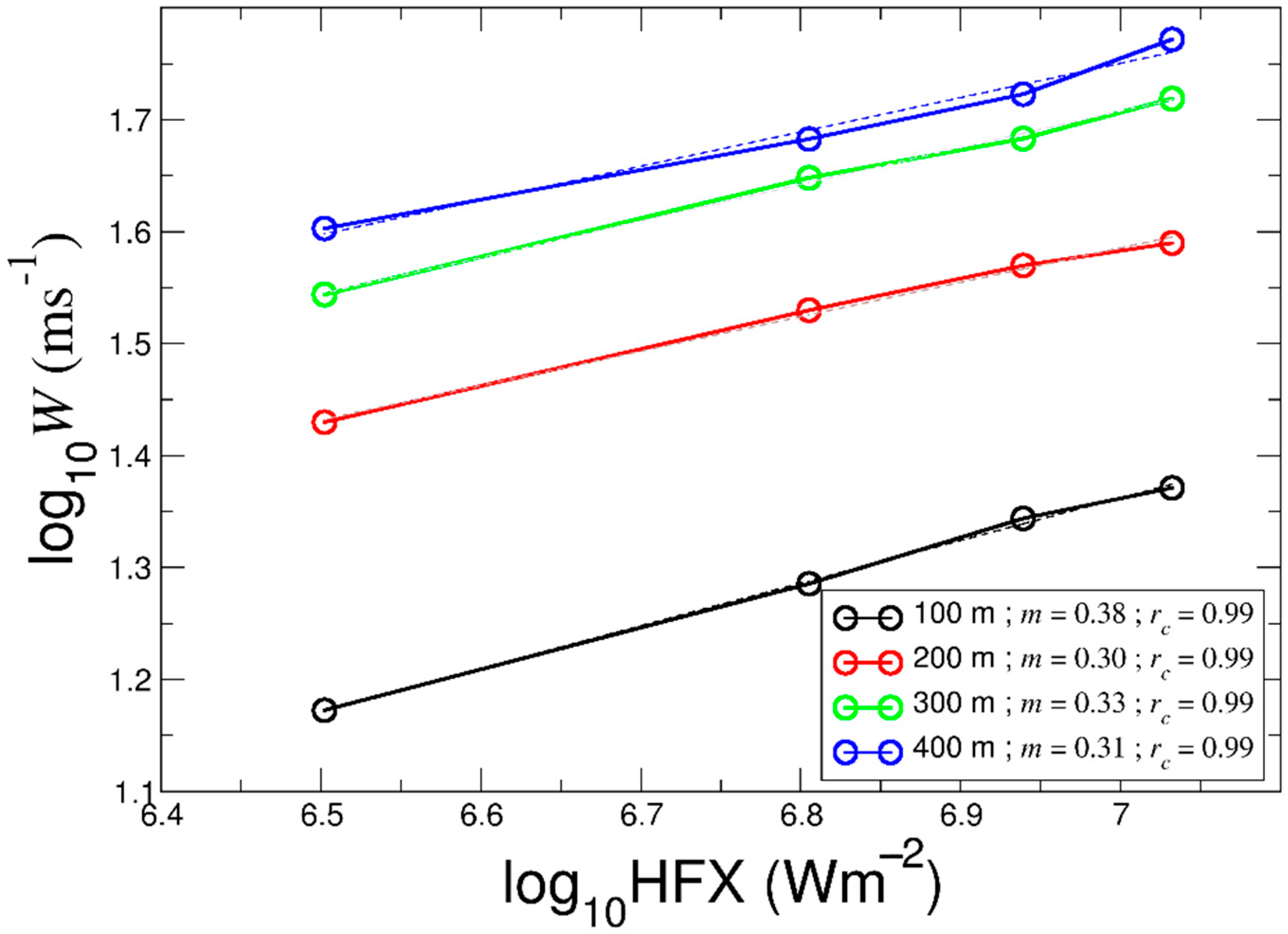
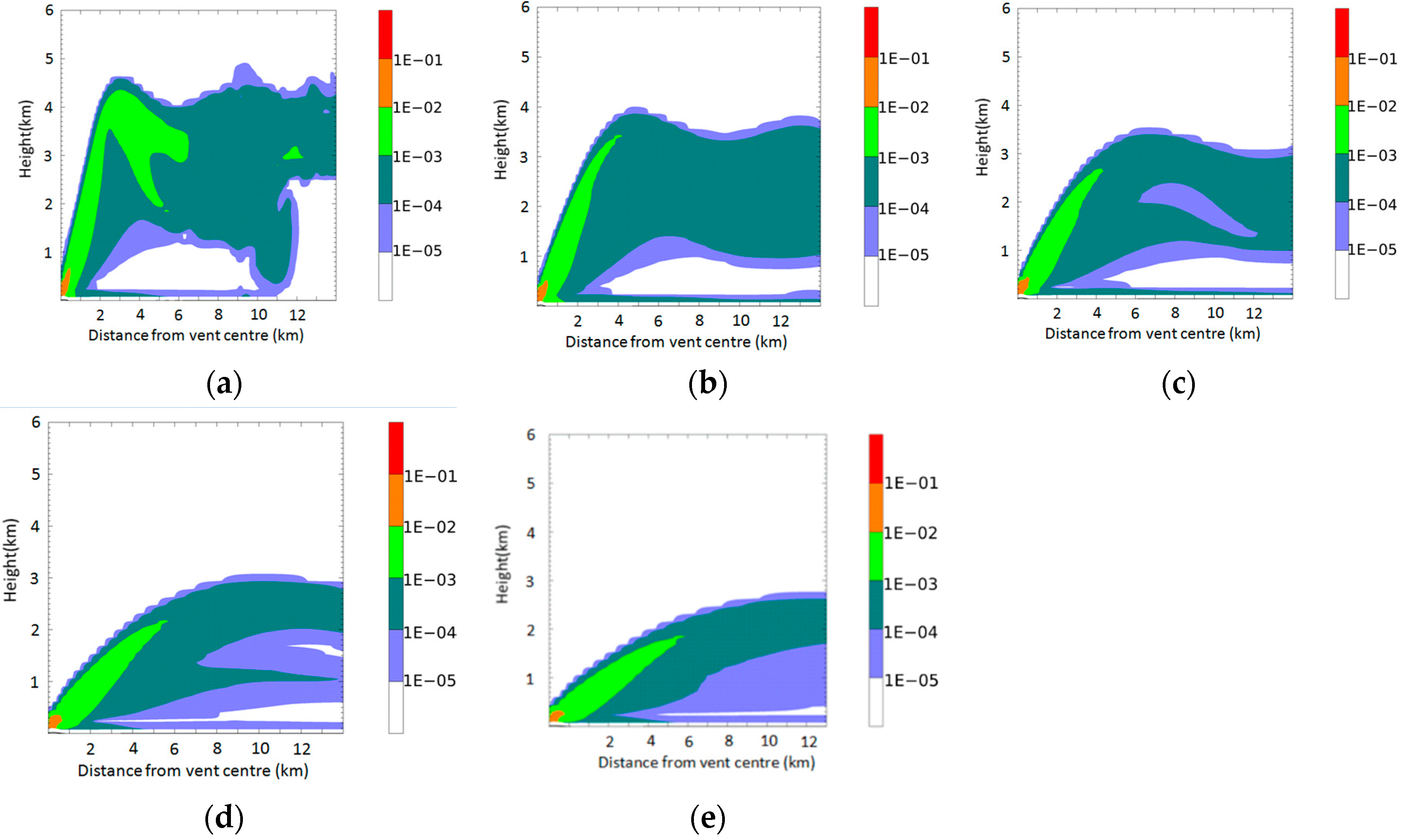
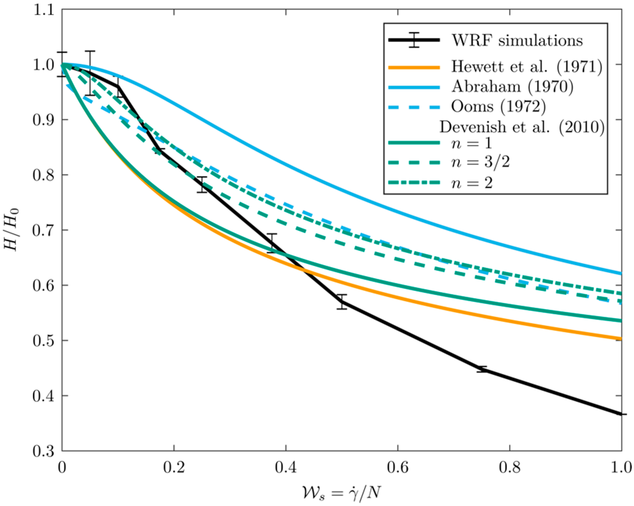
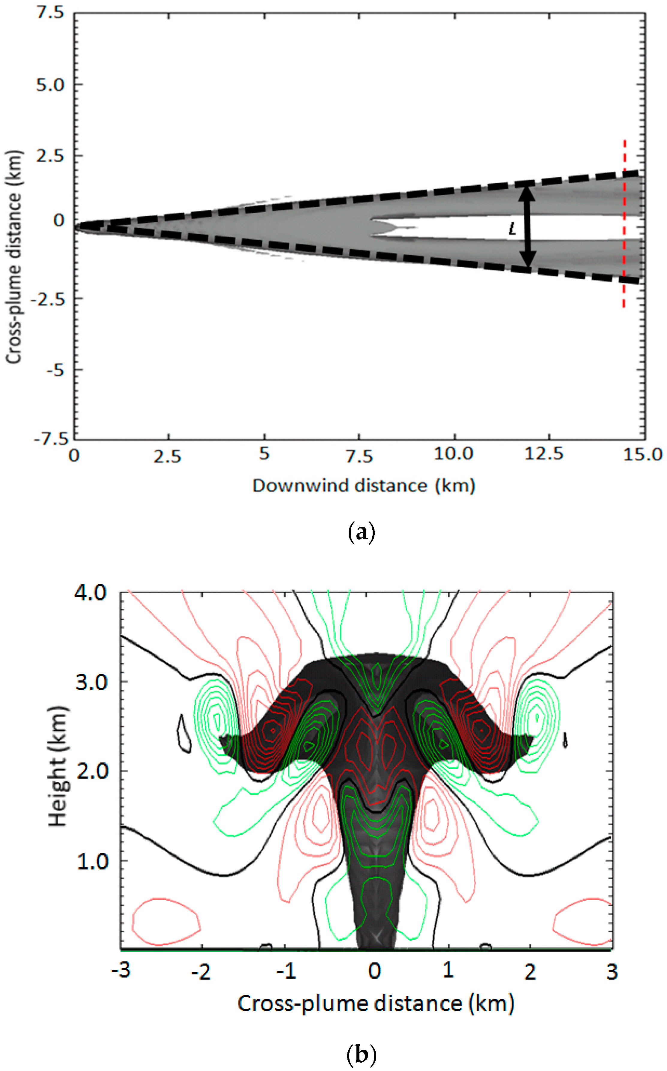
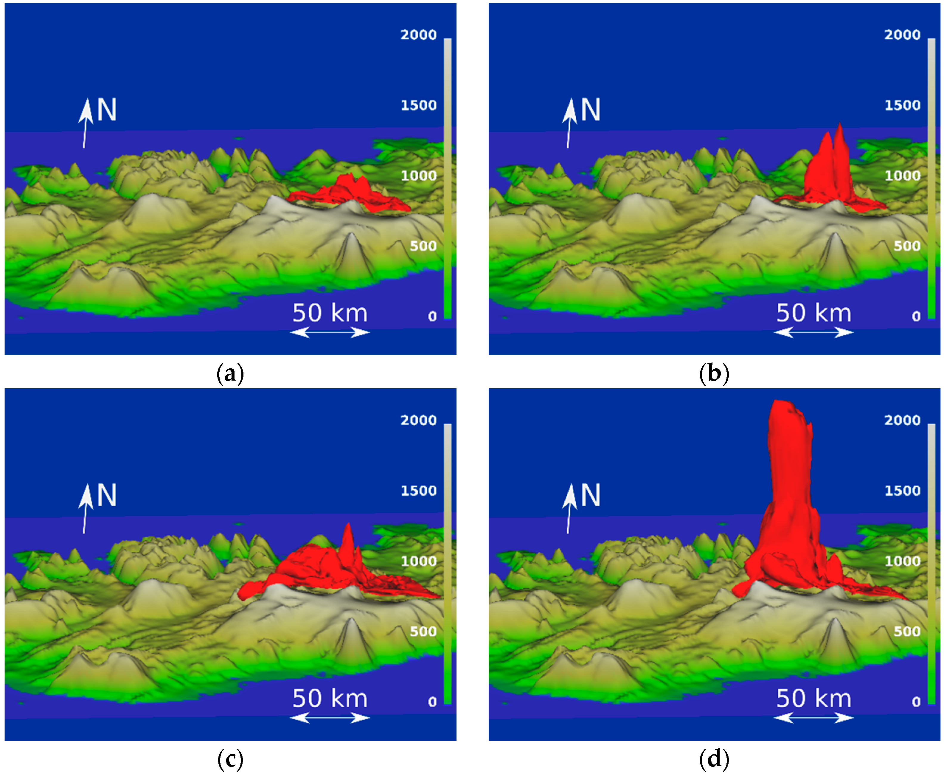
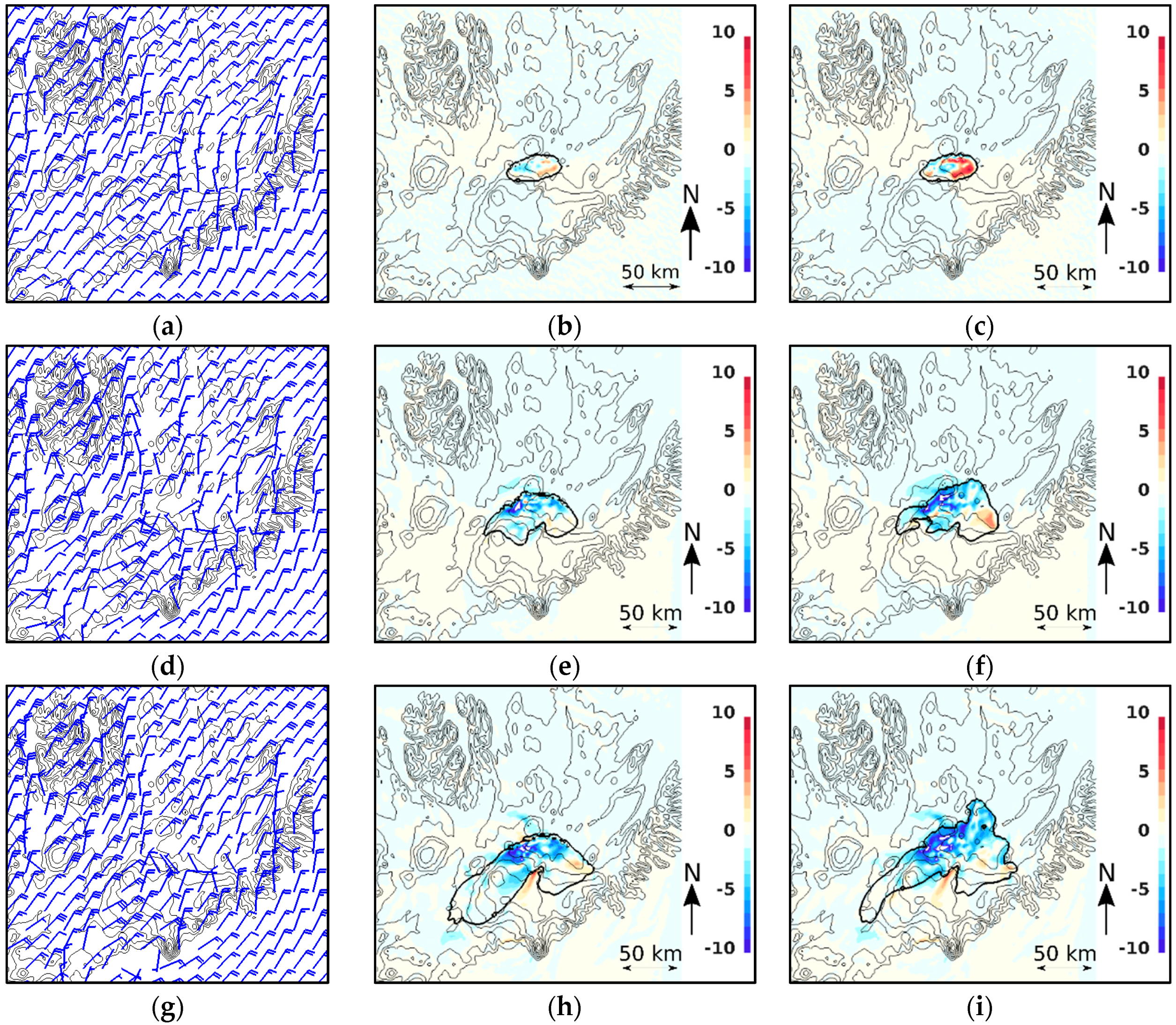
3.3. Bent over Plumes

The results presented above have adopted an atmosphere that is at rest. This is not the usual state of the atmosphere. Recently, there has been a renewed interest in plumes rising in a background wind field, following several volcanic eruptions (notably the 2010 eruption of Eyjafjallajökull, Iceland) where the plume was significantly influenced by atmospheric winds. Integral models of volcanic plumes that included a background wind field (e.g., [11,12,53]) have demonstrated that the rise height of plumes in a wind field is diminished in comparison to an equivalent source in a quiescent atmosphere. The neglect of the wind can then lead to very significant under-predictions of the source mass flux [12].
Explosive volcanic eruptions are often characterized as producing “strong plumes” or “weak plumes” on the basis of the effect of the background wind on the plume rise (e.g., [9]). Recent experimental work [54] has identified an intermediate “distorted plume” regime. The is wind-blown plume regimes are quantified using the dimensionless ratio of the wind speed to the plume velocity, here denoted by W and given by W = V / W = α 1 / 2 V / ( F 0 N ) 1 / 4 where F 0 = Q g R 2 ρ 0 c p T 0 is the buoyancy flux from the source [11,12]. For strong plumes, the background wind field has little influence on the plume ( W 1 ), whereas weak plumes are bent-over by the ambient wind. The distorted plume region (that separates these regimes) occurs for 0.11 < W < 0.37 , approximately, and is characterized by a sub-vertical rise to the neutral height with an overshoot regime that is downwind of the vent [54].
The reduction in the height of rise for plumes rising in a wind field indicates that the ambient wind enhances the mixing of atmospheric air into the plume. The density deficit that drives the vertical motion is therefore reduced more rapidly for wind-blown plumes. In integral models of turbulent buoyant plumes in a cross wind, the enhanced mixing is described by modifying the entrainment assumption of Morton et al. (1956). Several modified entrainment closures have been suggested, e.g., [14,38,55,56,57]. However, the calibration of these parameterizations of entrainment and turbulent mixing has been limited to settings that are accessible in the laboratory, which may differ from conditions found in the natural environment. For example, it is difficult to produce non-uniform velocity profiles in a moving density-stratified ambient to represent a windy atmosphere into which a volcano erupts, and therefore the wind entrainment parameterizations have commonly been calibrated in experiments adopting a uniform ambient flow. Numerical experiments provide an alternative to laboratory experiments.
In Figure 9, we present result from WRF simulations of plumes rising into a windy atmosphere. The wind field is prescribed on the upwind boundary of the domain as a linear shear profile. Figure 9a–e show that, when the background wind speed shear increases, the plume height is reduced as the plume bends over (cf. [12,53]). Figure 9a is reminiscent of distorted plumes observed in laboratory experiments in a uniform wind field [54] with the plume rising sub-vertically to the plume top height and the collapse to neutral buoyancy forms an intrusion that is swept downwind. On increasing the wind shear rate, the overshoot region is diminished, although the plume oscillates around the neutral buoyancy level (Figure 9b–e).
In Figure 10, we examine the effect of the wind on the maximum height of the plume (subsequently referred to as the plume height). The plume height is normalised by the height in the absence of wind (H0), and the wind shear rate is normalised by Brunt–Väisälä frequency, N, to give W s = γ ˙ / N which is the appropriate dimensionless parameter that characterizes the wind effect for a shear wind profile [12]. Figure 10 includes several predictions of the normalised plume height calculated using an integral plume model that adopts different entrainment closure models that have been proposed for wind-blown plumes [14,38,55,56] (see Appendix C). As shown in Figure 10, the WRF results fall within the envelope of theoretical results for W s < 0.4 , approximately. For values of W s above this, the present results indicate the plume height to be diminished more than is predicted by the integral models. Furthermore, the variation of the plume height for weak wind shear ( W s < 0.15 approximately) is markedly different from those of the integral plume model parameterizations, with the exception of the Abraham (1970) closure [55] (but this model does not well represent the plume height variation for larger dimensionless shear rates). If one of the theoretical models had to be chosen as closest to the present results (based upon root-mean square differences), it would be the Devenish et al. [38] three-parameter model. However, these results strongly suggest that none of plume entrainment parameterizations capture the entrainment dynamics observed in more complex environments. This is deserving of further research and, given the challenges of setting up such flows in the laboratory, numerical experiments are likely to be a valuable approach.
The WRF simulations are also capable of reproducing a further observed feature of wind-blown plumes: the bifurcation of the plume downwind of the vent [58]. In addition, for the weakest plumes in our simulations the plume bifurcates, and consists of buoyant vortex pairs. The bifurcation has been attributed to the development of lateral pressure gradients moving along the margins of the plume [9,58], which should be accompanied by a linear increase in vortex separation with distance. This type of linear separation can be seen in Figure 11a which shows a plan view of the plume, using an iso-surface of concentration used to visualize the plume margin, and it can be seen that the distance from plume axis to plume margin is approximately proportional to downwind distance. We note that in this simulation there are no “clear” regions between the bifurcating branches of the plume—merely substantially lowered concentrations. In Figure 11b, a cross-section through the plume downwind of the vent (at the distance noted on Figure 11a) is shown, with contours of the vertical velocity. The vortical motions can be inferred from the pattern of vertical velocities in Figure 11b. In addition to the central vortex pair, there are further, smaller eddies at the edge of the bifurcated plume. At the ground surface, at a cross-plume distance of 0 km, there is upward motion, flanked by downward motion at approximately 1.5 km AGL. This suggests a separate vortex pair in addition to the vortex pair associated with the stretching and tilting of vorticity near the plume source. Thus, these results show that the motion of the air in the vicinity of the plume is extremely complex.

4. More Complex Implementations

Example: Volcanic Degassing

Minor amendments to the WRF model used above could give further insight into the physical nature of the ash dispersal process. One possibility would be to add a negative velocity to the tracer elements, to mimic the effect of sedimentation. Such velocities may be obtained for atmospheric aerosols [59] based upon the mean free path, or for settling volcanic tephra [60]. This could be done by adding a settling velocity to the background velocity in the tracer-advection section of the code. This would require further study to demonstrate the validity and domain of applicability of the settling velocity assumptions, and there would be no simple scaling test for such a framework. This approach has not been taken further. Instead, a simpler approach to including the effect of negative buoyancy, one which agrees with theory and observations, is to add a dense gas to the model. This is achieved using the method of [43] where an extra microphysical mixing ratio (related to the concentration of the gas by the molar mixing ratio) is added to the WRF microphysical scheme to mimic, via the change in buoyancy, the effect of a dense gas, without interfering with the existing microphysics in any way. This method was shown to reproduce theoretical models of gravity current flow; for full details see [43]. A summary of the technical aspects is given in Appendix D. It should be stressed that, as in previous sections, no additional equations of motion were needed to produce this enhancement to the method.
The work in [43] showed how the modification could be used to simulate the spread of CO2 from a limnic eruption at Lake Nyos. Here, we show how the method could be used to simulate SO2 degassing from the Holuhraun fissure in Iceland, 2014–2015 as an example. The model is initialised with meteorological data from the National Centers for Environmental Prediction Global Forecast System (NCEP GFS) analyses [34] for 18 Z on the 2 November 2014, at which time the fissure was approximately 20 km long and 2 km wide (Figure 12) and was still emitting SO2. The model horizontal resolution used is 100 m, with underlying surface characteristics derived from a 30-arc-second database. A fissure surface heat flux of Q = 104 W m−2 was imposed along the Holuhraun fissure (see Figure 12). This magnitude of heat flux is typical of lava flows [61] and similar values have been used in other studies of the effect of lava heat flux on the atmosphere (e.g., [62]). Since the concentrations of the gases exsolved from the magma are not known precisely, we perform two simulations, using SO2 concentrations of 6 g kg−1 and 200 g kg−1 of gas. These concentrations are likely to be higher than those actually produced, but are included in order to stress-test this proof-of-concept approach. It should be emphasised that the motion of the volcanic fluid (dense gas plus ambient air) is now affecting the motion of the ambient air, as well as being affected by it. This is unlike chemical transport models (e.g., the chemistry version of WRF, WRF-CHEM) and thus the simulation is incorporating complex feedbacks between the volcanic gas and the ambient air.
The results of these simulations are illustrated in Figure 13, and show, in both cases, a buoyant plume rise during which entrainment of relatively dense atmospheric air reduces the density contrast, the cooling of the SO2 results in a mixture that is eventually more dense that the atmosphere, and the mixture collapses back to the ground, and spreads as a ground-hugging gravity current. This motion is strongly influenced by the wind field across the complex topography. As expected, the lighter gas (SO2 concentration of 6 g kg−1) reaches a higher altitude in the atmosphere (Figure 13, right-hand panels), with the cloud top approximately 8.5 km above ground level, while the denser gas (SO2 concentration of 200 g kg−1) reaches only approximately 4 km above ground level (Figure 13, left-hand panels). The horizontal spread of dense gas at the surface and lower levels is consequently greater, and the pollutant is seen to collect in the valleys (Figure 13f). Accompanying the spread of gas is a modification to the atmospheric flow. This can be seen in Figure 14 where the modification of the wind field due to the release of the pollutant is illustrated, showing that the footprint of the gas is clearly associated with changes to the flow of significant magnitude.
These results are intended only as an illustration of the WRF implementation and its potential application as a hazard model, since the fissure heat flux and release rates are unknown. However, the results demonstrate that the model can be modified to include the effects of orographic flow, dense volcanic gases and convection, and this may be useful for predicting the spread of volcanic gases in the event of a degassing episode, if the heat flux and source strength are known (or can be estimated). This was demonstrated in [63], a study of observed, elevated CO2 emissions from an unknown source on Katla volcano complex in Iceland. Firstly, many possible sources of CO2 were used in the dense gas simulations, and the source that produced results in agreement with the observations was selected as the potential source. Alongside this, an independent mass-flux model was used to estimate the emission rate from the source. Then the dense gas model was re-run, using the potential source and the emission rate from the mass-flux calculation. The simulated concentrations of CO2 (interpolated onto aircraft flight tracks) were found to be in very good agreement with the observations. The gas dispersion was found to be subject to complex patterns associated with the topography of Iceland and the model captured the observed spread of CO2 well for several cases with differing meteorological conditions.

5. Discussion

A method has been presented which allows near-field volcanic plume behaviour to be modelled via a standard (albeit state-of-the-art) numerical weather prediction model. Results have been presented which demonstrate that the model reproduces very well laboratory observations and theoretical predictions of various plume characteristics for idealised cases (using a passive tracer and no topography) for both the atmosphere at rest and for cases with background wind. The entrainment of unpolluted air into the modelled plume is in accord with the entrainment assumption across a range of times, heights, and surface forcings for plumes rising in a quiescent atmosphere.
For wind-blown plumes, our analysis has considered wind profiles that have a constant shear rate with height. This allows us to identify features that have been observed in laboratory tests. In applications to case studies of volcanic plumes, more complicated non-uniform velocity profile for the wind should be applied. This is straightforward in WRF, so WRF simulations allow an examination of the effects of shear in the wind velocity on the dynamics of the plume in a stratified atmosphere, an ambient setting that is extremely challenging to reproduce in the laboratory. The simulation of plumes using WRF can then be exploited as a surrogate for laboratory experimentation in the development and validation of mathematical models of turbulent buoyant plumes in atmospheric conditions that are difficult to reproduce in the laboratory.
The simulations we have performed show that parameterizations of entrainment into a wind-blown plume do not adequately describe the observed behaviour. As these entrainment models assume a uniform velocity profile, our results may indicate that the entrainment processes that occur for a plume rising in a shear flow differ from those in a uniform cross flow. This could have substantial implications as a shear profile is the generic condition in the lower atmosphere. Numerical simulations of the type used here parameterize sub-grid scale turbulence and therefore these results must be interpreted with some caution, although the reproduction of observed characteristics in quiescent atmospheres provides confidence in the sub-grid scheme. Further laboratory experiments and direct numerical simulation (where the turbulence is resolved down to the Kolmogorov microscale, requiring very high spatial and temporal resolution) is needed to understand the fundamental fluid dynamics of entrainment for plumes in stratified shear flows.

Limitations and Extensions of WRF Plume Modelling

In addition to a complex background wind and stratification profile, the simulation framework presented here provides an excellent means of examining the effect of more complex processes (such as microphysics) upon plume characteristics. Further developments are necessary to produce a model that is able to reproduce volcanic eruption columns where additional physical processes have a critical control on the dynamics.
The overly simple ‘volcanic source’ representation in our current model implementation (i.e., an areal source of buoyancy) neglects the mass and momentum that erupting volcanoes add to the atmosphere. Including a momentum flux at the source, by imposing a jet velocity at the lowest model level, is conceptually straightforward but high speeds require short time steps, as is typical for explicit numerical time-integration schemes. A non-zero mass flux at the source can be modelled, as illustrated in our dense gas application. Additionally, our dense gas application provides a framework for further developing the coupling between the erupted phase and the atmospheric air. For example, the microphysics scheme could be amended to alter the density of the erupted fluid to model pyroclast transport and their effect on the mixture density. These advances would develop this WRF framework towards a ‘dusty gas’ (also known as a ‘pseudogas’) eruption column model, whereby pyroclasts are idealized as being well-mixed through the eruption column and are in thermal and mechanical equilibrium with the surrounding gases, and therefore the mixture is modelled as a single phase with a density nonlinearly dependent on the mixing ratio. This approach has been found to be valid when the particle diameter of individual pyroclasts is no larger than 4 mm [5,64]. However, the majority of pyroclasts fall into this category [65]. Additionally, the equation of state for an ideal gas can be retained [5,35], as in the present study. Thus, the pseudogas approach has widespread application and has been successful when applied in integral models and CFD models.
The particle transport within an eruption column also influences the dynamics. The grain-size dependence of the settling speed of solid pyroclasts results in the larger clasts falling out of the column at lower altitudes than fine ash. Fallout removes mass and heat from the eruption column, and can strongly affect plume dynamics. Furthermore, the hazards posed by tephra make fallout a primary modelling concern; for proximal hazards the spatial distribution of fallout is essential, while for distal hazards to aviation the quantity and size-distribution of the ash fraction remaining aloft is required. The WRF modelling framework could in principle be extended to model the transport of several species, each modelled as a dense gas with its own mixing ratio and settling speed, with diagnostics extracted, at points for which these mixing ratios are non-zero, to determine the mixture density. This is feasible in WRF, but further work would be needed to see if this was possible in other NWP codes. This is not a truly multiphase model, but it may be possible to implement further extensions to model thermal disequilibrium between large clasts and the fine ash and gas mixture. Such developments would require careful testing.
A particularly intriguing aspect of eruption column dynamics is the two-way coupling of the plume with the atmosphere. Volcanic eruptions represent large perturbations to the atmosphere that can influence atmospheric dynamics in the proximal region (e.g., [35,66]). These atmospheric changes will feedback onto the plume dynamics. In modelling this two-way coupling, the use of an NWP model is invaluable.
As described above, the essence of our approach is to add an extra mixing ratio to the buoyancy module, without changing the pressure. This is straightforward in WRF. Further work would be needed to see if this can be done in other NWP codes, such as the Met Office Unified Model. That the pressure field does not need to be modified certainly makes this feasible. For operational NWP use, multiple WRF nests are commonly implemented: a finer-resolution domain is embedded within a lower-resolution domain, the two domains run synchronously. To include the methodology of this study, there could be two alternatives: (a) the dense gas (or pseudogas) method is applied only in the inner, high-resolution nest, or (b) the lower resolution nest supplies boundary conditions for an offline, high-resolution, single-domain dense-gas simulation. The same approach could presumably be used in other NWP models that use nests.

6. Conclusions

A weather forecasting model can be easily adapted to simulate volcanic eruptions and the subsequent spread of ash or gas. The numerical results are in good agreement with existing theory for plume rise in a quiescent atmosphere and capture observed features of wind-blown plumes. The simulations also suggest that parameterizations of entrainment into wind-blown plumes may not be applicable for non-uniform wind profiles. The model can easily be extended to simulate complex cases, such as the spread of heavy volcanic gases in regions of complex topography.
This approach has several advantages for ‘operational’ (and research) volcanic ash and gas transport modelling, including:
  • Providing a modelling framework that allows the plume dynamics and atmospheric dynamics to be modelled together.
  • Weather forecasting models often contain up-to-date representations of atmospheric physical processes and advanced numerical methods.
  • Weather forecasting models are under constant review, using extensive and varied observational datasets capturing a wide (and widening) range of atmospheric conditions.
  • Revision of weather forecasting models (often by extensive developer communities) reduces the development and maintenance burden of individual users.
  • Weather forecasting models are widely used and have established user communities providing mechanisms for support.
Further extensions will allow for other important physical processes that occur in volcanic eruption columns to be included.

Author Contributions

Conceptualization, all authors; Methodology, all authors; Software, R.R.B.; Validation, R.R.B. and M.J.W.; Formal Analysis, R.R.B. and M.J.W.; Investigation, all authors; Computing Resources, A.M.G. and R.R.B.; Data Curation, R.R.B.; Writing—Original Draft Preparation, all authors; Writing—Review & Editing, all authors; Visualization, R.R.B. and M.J.W.; Project Administration, S.D.M.; Funding Acquisition, S.D.M. All authors have read and agreed to the published version of the manuscript.

Funding

The authors would like to thank the UK Natural Environment Research Council (NERC) for funding this work via the VANAHEIM consortium (NERC Ref. NE/1015612/1).

Acknowledgments

We would like to thank Wei Wang of NCAR, USA for help and suggestions in configuring the WRF model to allow this work to be done. We would also like to thank the four anonymous reviewers whose helpful comments and suggestions have greatly improved this paper.

Conflicts of Interest

The authors declare no conflict of interest.

Appendix A

A comprehensive presentation of the WRF model equations is beyond the scope of this paper, but we present here (i) the main governing equations of motion—the flux-form Euler equations in a terrain-following coordinate system, and (ii) the principal equations governing the representation of turbulence. Note that most of this material is taken directly from [30], where all further details may be obtained, including the formulation of the moist Euler equations.

Appendix A.1. Flux-Form Euler Equations

Define V = μ v = ( U ,   V ,   W )   ;   Θ = μ θ where v = ( u ,   v ,   w ) are the velocities in the two horizontal and vertical directions and θ is the potential temperature, and μ is defined below. We denote the pressure by p, the geopotential by ϕ = g z and the inverse density by α = 1 / ρ .
The mass per unit area within a column is given by μ ( x ,   y ) = p h s p h t and the vertical coordinate is defined by η = ( p h p h t ) / μ where p h is the hydrostatic component of the pressure and p h s and p h t refer to the surface and top boundaries, respectively. This terrain-following system allows 0 η 1 . Then, the equations can be written as
t U + ( · V u ) x ( p ϕ η ) + μ   η ( p ϕ x ) = F U
t V + ( · V v ) y ( p ϕ η ) + η ( p ϕ y ) = F V
t W + ( · V w ) g ( η p μ ) = F W
t Θ + ( · V Θ ) = F Θ
t μ + ( · V ) = 0
t ϕ + μ 1 [ ( V · ϕ ) g W ] = 0
together with the relation
η ϕ = α μ
and the equation of state
p = p 0 ( R d θ / p 0 α ) γ
In the above, the subscripts x, y and η refer to differentiation; γ = c p / c v = 1.4 is the ratio of the heat capacities for dry air; R d is the gas constant for dry air; p 0 is a reference pressure, typically 105 Pascals. The forcing terms F U ,   F V and F W are associated with model physics, turbulent mixing, the use of map projections, and the rotation of the earth. For a full description of the governing equations, including the formulation of the moist flux-form Euler equations, the nature of the forcing terms, and the numerical solution of the equation set, see [30].

Appendix A.2. The 1.5-Order Turbulence Closure

In common with many other models, the full equations governing the evolution of turbulence cannot be implemented, and some degree of approximation is necessary to make the problem tractable. Such parametrisations are named according to the number of prognostic equations that are retained (see for example, [67]). Here, a one-and-a-half order turbulence kinetic energy (TKE) scheme is used, containing a prognostic equation for the evolution of TKE. The original formulation and parametrisation was provided by Yamada and Mellor [68]. The following contains a brief description of how the method is implemented in WRF.
In the presently used version of WRF, the equation governing the evolution of TKE e can be written as [30]
t ( μ e ) + ( · V e ) η = μ ( S + B + D )
where η and μ are the mass variables defined in Section Appendix A.1. The second term on the left-hand side of (A7) represents the transport of TKE. The right-hand-side of (A7) represents contributions from shear (S), buoyancy (B), and dissipation (D).
The shear term S is derived from the horizontal eddy viscosity K H , the vertical eddy viscosity K V , and the deformation tensor D by
S = K H D 11 2 + K H D 22 2 + K V D 33 2 + K h D 12 2 ¯ + K v D 13 2 ¯ + K v h D 23 2 ¯
and the overbars denote that a horizontal or vertical interpolator operator has been applied—see [30] for details. Also:
D 11 = 2 m x m y [ x ( m y 1 u ) z x z ( m y 1 u ) ]
D 22 = 2 m x m y [ y ( m x 1 v ) z y z ( m x 1 v ) ]
D 33 = 2 z w
D 12 = m x m y [ y ( m y 1 u ) z y z ( m y 1 u ) + x ( m x 1 v ) z x z ( m x 1 v ) ]
D 13 = m x m y [ x ( m y 1 w ) z x z ( m y 1 w ) ] + z ( u )
D 23 = m x m y [ y ( m y 1 w ) z y z ( m y 1 w ) ] + z ( v )
here, m x and m y are map factors relating the distance in computational space to the distance on the earth’s surface and z y and z x are geometric heights. The eddy viscosities K H and K V are defined as
K h , v = C l h , v e
where C is a constant in the range (0.15, 0.25) and l h , v are empirical length scales defined by:
l h , v = min [ ( Δ x Δ y Δ z ) 1 / 3 ,   0.76 e / N ]   for   N 2 > 0 ,
l h , v = ( Δ x Δ y Δ z ) 1 / 3   for   N 2 0
for grid spacings Δ x , Δ y and Δ z and Brunt-Väisälä frequency N.
The buoyancy term B is defined as
B = K V N 2
The dissipation term D is proportional to e 3 / 2   and also depends upon the mixing length, as defined in (A16) and (A17). For full details, see [30].

Appendix B.Summary of Important WRF Model Choices

The following table gives the principal WRF model choices made for the simulations contained in this study. They refer to diffusion, damping, boundary conditions, and surface heat flux. This information is primarily intended for WRF users, who may select the appropriate choice by means of the “namelist.input” file. The latter is split into sections. The relevant section is noted in Table A1 (column 2). For a full list of the choices available to the WRF user, see the WRF User Manual [40].
Table A1. The principal model choices, and their significance, used in this study.
Model Choice‘Namelist.Input’ SectionValue Used
tke_heat_flux&dynamics1500–9000 Kms−1(1)
diff_opt&dynamics2(2)
km_opt&dynamics2(3)
scalar_adv_opt&dynamics1(4)
mix_full_fields&dynamics1(5)
open_xs&bdy_control.true.(6)
open_xe&bdy_control.true.(6)
open_ys&bdy_control.true.(6)
open_ye&bdy_control.true.(6)
isfflx&physics2(7)
sf_sfclay_physics&physics1(8)
bl_pbl_physics&physics0(9)
(1) Note that heat flux is related to tke_heat_flux by the equation H = ρcp × tke_heat_flux where ρ is the density and cp is the specific heat capacity at constant pressure. (2) Compute horizontal diffusion in physical space rather than on model coordinate surfaces (more accurate when topography is present). (3) 1.5—order 3D TKE closure. (4) Positive-definite advection of scalars. (5) Vertical diffusion acts on full fields. (6) Open boundaries for x and y: starts (s) and end (e). (7) User supplies tke_heat_flux (see above), model determines friction velocity U*. (8) Monin-Obukhov similarity theory in surface layer. (9) Do not use a planetary boundary-layer parametrization.

Appendix C. Entrainment Parameterizations for Wind-Blown Plumes

There have been several parameterizations of turbulent entrainment into wind-blown plumes that extend the entrainment hypothesis of Morton et al. (1956) [15]. In this study, we compare the WRF simulations of the plume rise in a wind-field with integral models adopted one of four parameterizations for the entrainment velocity U e given below adopting a common notation whereby u is the axial velocity of the plume which has radius b , v is the uni-directional horizontal wind speed, and θ is the angle between the plume axis and the horizontal. Therefore, u sin θ is the vertical velocity of the plume, v cos θ is the component of the wind velocity along the plume axis, and v sin θ is the component of the wind velocity normal to the plume axis.
A commonly used entrainment parameterization is that of Hewett et al. (1971) [14],
U e = α | u v cos θ | + β | v sin θ | ,
which combines additively contributions to mixing due to relative velocities between the plume and the atmosphere in the axial and normal directions. This introduces two entrainment coefficients α and β , with α being identified with the entrainment coefficient of Morton et al. (1956) [15] (since equation A21 reduces to the entrainment hypothesis of [15] in the absence of wind), and β quantifies the additional entrainment that occurs due to the cross wind.
The parameterization of Abraham (1970) [55] is
U e = α | u v cos θ | + β | v sin θ | cos θ ,
is similar to that of Hewett et al. (1971) [14], but includes an ad-hoc factor on the wind entrainment contribution to remove this effect for vertically rising plumes.
Ooms (1972) [56] adds a further extension to the parameterization of Abraham (1970) [55], including a contribution modelling enhanced mixing due to atmospheric turbulence in the wind field,
U e = α | u v cos θ | + β | v sin θ | cos θ + ( ϵ b ) 1 / 3 ,
where ϵ denote the atmospheric eddy energy dissipation which can be modelled as linearly dependent on the wind speed, ϵ 2 × 10 4 v .
Devenish et al. (2010) [38] introduce an alternative model, whereby the contributions of the wind and the axial shear are combined non-linearly. Additionally, Devenish et al. (2010) [38] assume that the horizontal speed of the plume adjusts very rapidly to the wind speed, so that the axial velocity of the plume is given by | u sin θ | 2 + v 2 , resulting in a three-parameter model,
U e = | u sin θ | | u sin θ | 2 + v 2 [ ( α | u sin θ | ) n + ( β v ) n ] 1 / n ,
where n is an empirical parameter. For n = 1 an additive contribution of each effect is recovered. On the basis of LES simulations, Devenish et al. (2010) [38] propose that values of n = 3 / 2 or n = 2 are better at reproducing observed plume dynamics than the simple additive model.
The entrainment coefficients α and β are calibrated using laboratory experiments, field scale observations (e.g., of plumes from industrial smokestacks) and numerical simulations. The range of variation on α is typically much smaller than that for β , although both parameters are uncertain. When comparing the WRF simulations to integral models adopting these entrainment parameterizations (Figure 10) we take typical values, with α = 0.1 and β = 0.5 .

Appendix D. Dense Gas Model

In order to simulate the release of a dense gas (in Section 4), the method of Burton et al. [43] was adopted. At the release location, a specified mixing ratio q G A S (in kg kg−1) of gas is introduced into the model (by means of the Registry file, plus recompilation). This mixing ratio is then passed to all other model subroutines where buoyancy is evaluated, and if q G A S > 0 kg kg−1 then the buoyancy will be affected. Note that this does not require the addition of any further equations to the model equation set, and this modification is very straightforward to implement, associated with the modular WRF software design. Essentially, this corresponds to changing the density of an air parcel. From [30] if α d is the inverse density of dry air, then the inverse density, taking into account the full parcel density, is given by α = α d ( 1 + i = 1 M q i + q G A S ) 1 where q1, q2, …, qM are the M microphysical mixing ratios (corresponding to water vapour, cloud, ice, etc.). M may vary depending upon which microphysical scheme is being used. It should be noted that the gas mixing ratio q G A S   does not interact with the microphysics per se, but merely acts to reduce the buoyancy. In the default version of WRF, α = α d ( 1 + i = 1 M q i ) 1 .
Physically, this approach is equivalent to replacing molecules of oxygen (for example) in a reference volume with molecules of dense gas, one-for-one. Then, from the equation of state P V = n R T , where n is the number of molecules, the pressure does not change. In reality the gas constant R would change, of course, adding a source of potential temperature, but (as in [43]) this effect is estimated to be insignificant, and to make the problem tractable, we have not included it. Note that in the pseudogas approach the particulate matter contribution to the gas constant (for small diameter particles) can be neglected [5], giving wider application to this method.
In practice, there are three steps to implementing the dense gas release: (i) the extra mixing ratio is introduced into the model framework, as described above; (ii) the source release location is specified in the code (in the microphysics driver routine); (iii) the heat flux is specified at the same locations as in (ii)—see Table A1 (Appendix B) for the heat flux model choices. As mentioned in the main body of the text, the specification of a fixed release rate of gas can also be implemented, as in [63].

References

  1. Jones, A.; Thomson, D.; Hort, M.; Devenish, B. The U.K. Met Office’s Next-Generation Atmospheric Dispersion Model, NAME III. In Air Pollution Modeling and Its Application XVII; Borrego, C., Norman, A.-L., Eds.; Springer: Boston, MA, USA, 2007; pp. 580–589. [Google Scholar]
  2. Folch, A.; Costa, A.; Macedonio, G. FALL3D: A computational model for transport and deposition of volcanic ash. Comput. Geosci. 2009, 35, 1334–1342. [Google Scholar] [CrossRef]
  3. Schwaiger, H.F.; Denlinger, R.P.; Mastin, L.G. Ash3d: A finite-volume, conservative numerical model for ash transport and tephra deposition. J. Geophys. Res. Solid Earth 2012, 117, B04204. [Google Scholar] [CrossRef]
  4. Oberhuber, J.M.; Herzog, M.; Graf, H.-F.; Schwanke, K. Volcanic plume simulation on large scales. J. Volcanol. Geotherm. Res. 1998, 87, 29–53. [Google Scholar] [CrossRef] [Green Version]
  5. Suzuki, Y.J.; Koyaguchi, T.; Ogawa, M.; Hachisu, I. A numerical study of turbulent mixing in eruption clouds using a three-dimensional fluid dynamics model. J. Geophys. Res. Solid Earth 2005, 110. [Google Scholar] [CrossRef]
  6. Esposti Ongaro, T.; Cavazzoni, C.; Erbacci, G.; Neri, A.; Salvetti, M.V. A parallel multiphase flow code for the 3D simulation of explosive volcanic eruptions. Parallel Computing 2007, 33, 541–560. [Google Scholar] [CrossRef]
  7. Cerminara, M.; Esposti Ongaro, T.; Berselli, L.C. ASHEE-1.0: A compressible, equilibrium–Eulerian model for volcanic ash plumes. Geosci. Model Dev. 2016, 9, 697–730. [Google Scholar] [CrossRef] [Green Version]
  8. Suzuki, Y.J.; Costa, A.; Cerminara, M.; Esposti Ongaro, T.; Herzog, M.; Van Eaton, A.R.; Denby, L.C. Inter-comparison of three-dimensional models of volcanic plumes. J. Volcanol. Geotherm. Res. 2016, 326, 26–42. [Google Scholar] [CrossRef] [Green Version]
  9. Sparks, R.S.J.; Bursik, M.I.; Carey, S.N.; Gilbert, J.S.; Glaze, L.; Sigurdsson, H.; Woods, A.W. Volcanic Plumes; Wiley: Chichester, UK, 1997. [Google Scholar]
  10. Mastin, L.G.; Guffanti, M.; Servranckx, R.; Webley, P.; Barsotti, S.; Dean, K.; Durant, A.; Ewert, J.W.; Neri, A.; Rose, W.I.; et al. A multidisciplinary effort to assign realistic source parameters to models of volcanic ash-cloud transport and dispersion during eruptions. J. Volcanol. Geotherm. Res. 2009, 186, 10–21. [Google Scholar] [CrossRef]
  11. Degruyter, W.; Bonadonna, C. Improving on mass flow rate estimates of volcanic eruptions. Geophys. Res. Lett. 2012, 39, L16308. [Google Scholar] [CrossRef] [Green Version]
  12. Woodhouse, M.J.; Hogg, A.J.; Phillips, J.C.; Sparks, R.S.J. Interaction between volcanic plumes and wind during the 2010 Eyjafjallajökull eruption, Iceland. J. Geophys. Res. Solid Earth 2013, 118, 92–109. [Google Scholar] [CrossRef] [Green Version]
  13. Aubry, T.J.; Jellinek, A.M.; Carazzo, G.; Gallo, R.; Hatcher, K.; Dunning, J. A new analytical scaling for turbulent wind-bent plumes: Comparison of scaling laws with analog experiments and a new database of eruptive conditions for predicting the height of volcanic plumes. J. Volcanol. Geotherm. Res. 2017, 343, 233–251. [Google Scholar] [CrossRef]
  14. Hewett, T.A.; Fay, J.A.; Hoult, D.P. Laboratory experiments of smokestack plumes in a stable atmosphere. Atmos. Environ. 1971, 5, 767–789. [Google Scholar] [CrossRef]
  15. Morton, B.R.; Taylor, G.I.; Turner, J.S. Turbulent gravitational convection from maintained and instantaneous sources. Proc. Roy. Soc. London, Ser. A 1956, 234, 1–23. [Google Scholar] [CrossRef]
  16. Woods, A.W. The fluid dynamics and thermodynamics of eruption columns. Bull. Volcanol. 1988, 50, 169–193. [Google Scholar] [CrossRef]
  17. Costa, A.; Suzuki, Y.J.; Cerminara, M.; Devenish, B.J.; Ongaro, T.E.; Herzog, M.; Van Eaton, A.R.; Denby, L.C.; Bursik, M.; de’ Michieli Vitturi, M.; et al. Results of the eruptive column model inter-comparison study. J. Volcanol. Geotherm. Res. 2016, 326, 2–25. [Google Scholar] [CrossRef] [Green Version]
  18. Woodhouse, M.J.; Hogg, A.J.; Phillips, J.C.; Rougier, J.C. Uncertainty analysis of a model of wind-blown volcanic plumes. Bull. Volcanol. 2015, 77, 83. [Google Scholar] [CrossRef]
  19. Marti, A.; Folch, A.; Jorba, O.; Janjic, Z. Volcanic ash modeling with the online NMMB-MONARCH-ASH v1.0 model: Model description, case simulation, and evaluation. Atmos. Chem. Phys. 2017, 17, 4005–4030. [Google Scholar] [CrossRef] [Green Version]
  20. Poulidis, A.P.; Phillips, J.C.; Renfrew, I.A.; Barclay, J.; Hogg, A.; Jenkins, S.F.; Robertson, R.; Pyle, D.M. Meteorological Controls on Local and Regional Volcanic Ash Dispersal. Scientific Reports 2018, 8, 6873. [Google Scholar] [CrossRef]
  21. Watt, S.F.L.; Gilbert, J.S.; Folch, A.; Phillips, J.C.; Cai, X.M. An example of enhanced tephra deposition driven by topographically induced atmospheric turbulence. Bull. Volcanol. 2015, 77, 35. [Google Scholar] [CrossRef] [Green Version]
  22. Poulidis, A.P.; Takemi, T.; Iguchi, M.; Renfrew, I.A. Orographic effects on the transport and deposition of volcanic ash: A case study of Mount Sakurajima, Japan. J. Geophys. Res. Atmos. 2017, 122, 9332–9350. [Google Scholar] [CrossRef]
  23. Neri, A.; Esposti Ongaro, T.; Macedonio, G.; Gidaspow, D. Multiparticle simulation of collapsing volcanic columns and pyroclastic flow. J. Geophys. Res. Solid Earth 2003, 108, 2202. [Google Scholar] [CrossRef]
  24. Costa, A.; Suzuki, Y.; Folch, A.; Cioni, R. Numerical models of volcanic eruption plumes: Inter-comparison and sensitivity. J. Volcanol. Geotherm. Res. 2016, 326, 1. [Google Scholar] [CrossRef]
  25. Cao, Z.; Patra, A.; Bursik, M.; Pitman, E.B.; Jones, M. Plume-SPH 1.0: A three-dimensional, dusty-gas volcanic plume model based on smoothed particle hydrodynamics. Geosci. Model Dev. 2018, 11, 2691–2715. [Google Scholar] [CrossRef] [Green Version]
  26. Heinold, B.; Tegen, I.; Wolke, R.; Ansmann, A.; Mattis, I.; Minikin, A.; Schumann, U.; Weinzierl, B. Simulations of the 2010 Eyjafjallajökull volcanic ash dispersal over Europe using COSMO–MUSCAT. Atmos. Environ. 2012, 48, 195–204. [Google Scholar] [CrossRef] [Green Version]
  27. Grell, G.A.; Peckham, S.E.; Schmitz, R.; McKeen, S.A.; Frost, G.; Skamarock, W.C.; Eder, B. Fully coupled “online” chemistry within the WRF model. Atmos. Environ. 2005, 39, 6957–6975. [Google Scholar] [CrossRef]
  28. Stuefer, M.; Freitas, S.R.; Grell, G.; Webley, P.; Peckham, S.; McKeen, S.A.; Egan, S.D. Inclusion of ash and SO2 emissions from volcanic eruptions in WRF-Chem: Development and some applications. Geosci. Model Dev. 2013, 6, 457–468. [Google Scholar] [CrossRef] [Green Version]
  29. Ahmadov, R.; Peckham, S.; Grell, G.; Pagowski, M.; McKeen, S.; Barth, M.; Wiedinmyer, C.; Pfister, G.; Kumar, R.; Knote, C.; et al. Best Practices for Applying WRF-Chem 3.8.1. Available online: https://ruc.noaa.gov/wrf/wrf-chem/wrf_tutorial_2017/Best_Practices.pdf (accessed on 16 April 2020).
  30. Skamarock, W.C.; Klemp, J.B.; Dudhia, J.; Gill, D.O.; Barker, O.M.; Wang, W.; Powers, J.G. A description of the Advanced Research WRF Version 2. In NCAR Tech Notes-468+STR. 2005. Available online: https://opensky.ucar.edu/islandora/object/technotes:479 (accessed on 16 April 2020). [CrossRef]
  31. Weather Research and Forecasting Model. Available online: https://www.mmm.ucar.edu/weather-research-and-forecasting-model (accessed on 16 April 2020).
  32. Powers, J.G.; Klemp, J.B.; Skamarock, W.C.; Davis, C.A.; Dudhia, J.; Gill, D.O.; Coen, J.L.; Gochis, D.J.; Ahmadov, R.; Peckham, S.E.; et al. The Weather Research and Forecasting Model: Overview, System Efforts, and Future Directions. Bull. Am. Meteorol. Soc. 2017, 98, 1717–1737. [Google Scholar] [CrossRef]
  33. Fernando, H.J.S. Handbook of Environmental Fluid Dynamics; Taylor & Francis: Boca Raton, FL, USA, 2013. [Google Scholar]
  34. NCEP-GFS. Available online: https://www.ncdc.noaa.gov/data-access/model-data/model-datasets/global-forcast-system-gfs (accessed on 16 April 2020).
  35. Poulidis, A.P.; Renfrew, I.A.; Matthews, A.J. Thermally Induced Convective Circulation and Precipitation over an Isolated Volcano. J. Atmos. Sci. 2016, 73, 1667–1686. [Google Scholar] [CrossRef] [Green Version]
  36. Innes, P.; Dorling, S. Operational Weather Forecasting; Wiley-Blackwell: London, UK, 2013. [Google Scholar]
  37. Elghobashi, S. On predicting particle-laden turbulent flows. Appl. Sci. Res. 1994, 52, 309–329. [Google Scholar] [CrossRef]
  38. Devenish, B.J.; Rooney, G.G.; Webster, H.N.; Thomson, D.J. The Entrainment Rate for Buoyant Plumes in a Crossflow. Boundary Layer Meteorol. 2010, 134, 411–439. [Google Scholar] [CrossRef]
  39. Arakawa, A.; Lamb, V.R. Computational Design of the Basic Dynamical Processes of the UCLA General Circulation Model. In Methods in Computational Physics: Advances in Research and Applications; Chang, J., Ed.; Elsevier: New York, NY, USA, 1977; Volume 17, pp. 173–265. [Google Scholar]
  40. User’s Guides for the Advanced Research WRF (ARW) Modeling System, Version 3. Available online: https://www2.mmm.ucar.edu/wrf/users/docs/user_guide_V3/contents.html (accessed on 16 April 2020).
  41. U.S. Standard Atmosphere; U.S. Government Printing Office: Washington, DC, USA, 1976.
  42. Sparks, R.S.J. The dimensions and dynamics of volcanic eruption columns. Bull. Volcanol. 1986, 48, 3–15. [Google Scholar] [CrossRef]
  43. Burton, R.R.; Dudhia, J.; Gadian, A.M.; Mobbs, S.D. The use of a numerical weather prediction model to simulate the release of a dense gas with an application to the Lake Nyos disaster of 1986. Meteorol. Appl. 2017, 24, 43–51. [Google Scholar] [CrossRef] [Green Version]
  44. Turner, J.S. Buoyancy Effects in Fluids; Cambridge University Press: Cambridge, UK, 1973. [Google Scholar]
  45. Morton, B.R.; Middleton, J. Scale diagrams for forced plumes. J. Fluid Mech. 1973, 58, 165–176. [Google Scholar] [CrossRef]
  46. Hunt, G.R.; Kaye, N.B. Lazy plumes. J. Fluid Mech. 2005, 533, 329–338. [Google Scholar] [CrossRef]
  47. Devenish, B.J.; Edwards, J.M. Large-eddy simulation of the plume generated by the fire at the Buncefield oil depot in December 2005. Proc. Roy. Soc. London, Ser. A 2009, 465, 397–419. [Google Scholar] [CrossRef]
  48. Batchelor, G.K. Heat convection and buoyancy effects in fluids. Q. J. Roy. Meteorol. Soc. 1954, 80, 339–358. [Google Scholar] [CrossRef]
  49. Kaminski, E.; Tait, S.; Carazzo, G. Turbulent entrainment in jets with arbitrary buoyancy. J. Fluid Mech. 2005, 526, 361–376. [Google Scholar] [CrossRef] [Green Version]
  50. Ezzamel, A.; Salizzoni, P.; Hunt, G.R. Dynamical variability of axisymmetric buoyant plumes. J. Fluid Mech. 2015, 765, 576–611. [Google Scholar] [CrossRef]
  51. Papanicolaou, P.N.; List, E.J. Investigations of round vertical turbulent buoyant jets. J. Fluid Mech. 1988, 195, 341–391. [Google Scholar] [CrossRef]
  52. List, E.J. Turbulent Jets and Plumes. Annu. Rev. Fluid Mech. 1982, 14, 189–212. [Google Scholar] [CrossRef]
  53. Bursik, M. Effect of wind on the rise height of volcanic plumes. Geophys. Res. Lett. 2001, 28, 3621–3624. [Google Scholar] [CrossRef] [Green Version]
  54. Carazzo, G.; Girault, F.; Aubry, T.; Bouquerel, H.; Kaminski, E. Laboratory experiments of forced plumes in a density-stratified crossflow and implications for volcanic plumes. Geophys. Res. Lett. 2014, 41, 8759–8766. [Google Scholar] [CrossRef]
  55. Abraham, G. The Flow of Round Buoyant Jets Issuing Vertically into Ambient Fluid Flowing in a Horizontal Direction; Delft Hydraulics Laboratory: Delft, The Netherlands, 1971. [Google Scholar]
  56. Ooms, G. A new method for the calculation of the plume path of gases emitted by a stack. Atmos. Environ. 1972, 6, 899–909. [Google Scholar] [CrossRef]
  57. Contini, D.; Donateo, A.; Cesari, D.; Robins, A.G. Comparison of plume rise models against water tank experimental data for neutral and stable crossflows. J. Wind Eng. Ind. Aerodyn. 2011, 99, 539–553. [Google Scholar] [CrossRef]
  58. Ernst, G.G.J.; Davis, J.P.; Sparks, R.S.J. Bifurcation of volcanic plumes in a crosswind. Bull. Volcanol. 1994, 56, 159–169. [Google Scholar] [CrossRef]
  59. Kasten, F. Falling Speed of Aerosol Particles. J. Appl. Meteorol. 1968, 7, 944–947. [Google Scholar] [CrossRef] [Green Version]
  60. Wilson, L.; Huang, T.C. The influence of shape on the atmospheric settling velocity of volcanic ash particles. Earth Planet. Sci. Lett. 1979, 44, 311–324. [Google Scholar] [CrossRef]
  61. Rowland, S.K.; Garbeil, H.; Harris, A.J.L. Lengths and hazards from channel-fed lava flows on Mauna Loa, Hawai‘i, determined from thermal and downslope modeling with FLOWGO. Bull. Volcanol. 2005, 67, 634–647. [Google Scholar] [CrossRef]
  62. Durand, J.; Tulet, P.; Leriche, M.; Bielli, S.; Villeneuve, N.; Muro, A.D.; Fillipi, J.-B. Modeling the lava heat flux during severe effusive volcanic eruption: An important impact on surface air quality. J. Geophys. Res. Atmos. 2014, 119, 11729–11742. [Google Scholar] [CrossRef] [Green Version]
  63. Ilyinskaya, E.; Mobbs, S.; Burton, R.; Burton, M.; Pardini, F.; Pfeffer, M.A.; Purvis, R.; Lee, J.; Bauguitte, S.; Brooks, B.; et al. Globally Significant CO2 Emissions From Katla, a Subglacial Volcano in Iceland. Geophys. Res. Lett. 2018, 45, 10332–10341. [Google Scholar] [CrossRef] [Green Version]
  64. Woods, A.W.; Bursik, M.I. Particle fallout, thermal disequilibrium and volcanic plumes. Bull. Volcanol. 1991, 53, 559–570. [Google Scholar] [CrossRef]
  65. Sparks, R.S.J.; Wilson, L. A model for the formation of ignimbrite by gravitational column collapse. J. Geol. Soc. 1976, 132, 441–451. [Google Scholar] [CrossRef]
  66. Tupper, A.; Textor, C.; Herzog, M.; Graf, H.-F.; Richards, M.S. Tall clouds from small eruptions: The sensitivity of eruption height and fine ash content to tropospheric instability. Nat. Hazards 2009, 51, 375–401. [Google Scholar] [CrossRef]
  67. Stull, R.B. An Introduction to Boundary Layer Meteorology; Kluwer Academic Publishers: Dordrecht, The Netherlands, 1988. [Google Scholar]
  68. Yamada, T.; Mellor, G. A Simulation of the Wangara Atmospheric Boundary Layer Data. J. Atmos. Sci. 1975, 32, 2309–2329. [Google Scholar] [CrossRef] [Green Version]
Figure 1. Dependence of plume height log H upon associated surface heat flux Q. The line of best fit connecting the simulated heights is marked with a dotted line and the inset text shows the gradient (m) and correlation coefficient (rc) for this best-fit line.
Atmosphere 11 00594 g001
Figure 2. Structure of plume at t = 1200 s. (a) An isosurface of constant arbitrary concentration; (b) ejection column showing concentration (colour shaded; arbitrary units). In (b) a dashed line represents a distance/height gradient of 0.11.
Atmosphere 11 00594 g002
Figure 3. Maximum vertical velocities within the plume, W , at several heights above ground level for increasing surface heat flux, H F X . The best linear fit (denote by dashed lines, with gradient m and correlation coefficient rc) is also shown for each group of simulations.
Atmosphere 11 00594 g003
Figure 4. (a) The mean centre-line vertical velocity WMEAN as a function of height; (b) the profile of difference between root-mean square vertical velocity WRMS and WMEAN as a function of height, indicating regions of enhanced turbulence. Both plots use time averaging.
Atmosphere 11 00594 g004
Figure 5. Vertical velocity in plume ejection column for vent heat flux density Q = 1.8 × 10⁶ W m−2, 30 min after eruption. Individual panels represent various heights above ground (denoted in each panel).
Atmosphere 11 00594 g005
Figure 6. Radial spread against height for (a) 15, (b) 30, (c) 45 and (d) 60 min after eruption. Symbols represent vent heat fluxes of Q = 1.8 × 10⁶ W m−2 (circles), Q = 6.4 × 10⁶ W m−2 (diamonds), Q = 8.8 × 10⁶ W m−2 (squares), Q = 1.1 × 10⁷ W m−2 (stars). The best-line fit (see text for properties) for all the data is shown by the solid black line.
Atmosphere 11 00594 g006
Figure 7. Velocity of entrained air U(x, z, t) normalised by maximum plume velocity WMAX(z, t) (where z is altitude and t is time) against normalised distance from vent (γ0 (z, t) is Gaussian plume width). Plots show results for 15 min (black lines), 30 min (red lines), 45 min (green lines) and 60 min (blue lines) after eruption. Surface forcing is Q = 1.1 × 10⁷ W m−2. The altitude at which the analysis is performed for is inset in each plot.
Atmosphere 11 00594 g007
Figure 8. The mean of all the curves shown in Figure 7 (solid black line). The equivalent mean for a surface forcing of Q = 4.4 × 10⁶ W m−2 is also shown (dotted black line). The red, green and black thin solid lines represent the expected theoretical variation for three values of entrainment coefficient (see text for details).
Atmosphere 11 00594 g008
Figure 9. Dependence of plume height for background wind speeds (constant shear rate) of (a) 1 × 10⁻³ s−1, (b) 1.5 × 10⁻³ s−1, (c) 2 × 10⁻³ s−1, (d) 3 × 10⁻³ s−1 and (e) 4 × 10⁻³ s−1. Results are for t = 1200 s after eruption. The non-dimensional values of W (see text) are (a) 0.1, (b) 0.15, (c) 0.2, (d) 0.3 and (e) 0.4.
Atmosphere 11 00594 g009
Figure 10. Normalised plume height as a function of the normalised shear W s for WRF results and an integral model adopting different entrainment parameterizations (see Appendix C and references shown in the legend). Error bars on the WRF results show ±1 standard deviation in the temporally varying height. H0 is the height in the absence of wind shear. The atmosphere is stably stratified with the Brunt-Väisälä frequency N = 0.01   s 1 .
Atmosphere 11 00594 g010
Figure 11. (a) Iso-surface of concentration at t = 1200 s for background wind speed of 5 ms−1 looking down on the plume. The straight black dotted line shows the near-linear spread of the plume edge, the distance L being a near-linear function of downwind distance; the red dotted line corresponds to the cross section shown in Figure 11b. (b) A cross-section through the plume, in the plane with normal aligned with the wind direction, indicated by the red-dashed line in Figure 11a. The area within an iso-surface of concentration, representing the plume edge, is shaded. Contours of the vertical velocity (red, negative; green, positive; solid black, zero) are shown.
Atmosphere 11 00594 g011
Figure 12. Topography of Iceland (coastline in solid blue line) with elevation contour intervals every 100 m; the solid black shaded area represents the Holuhraun fissure.
Atmosphere 11 00594 g012
Figure 13. Visualisation of the spread of SO2 from Holuraun fissure, November 2014. The 1 g kg−1 SO2 mixing ratio is shown in red, for gas release rates of 200 g kg−1 for (a) 20 min, (c) 60 min and (e) 120 min after eruption. (b,d,f show the same times after eruption, but are for a release rate of 6 g kg−1. The viewpoint is from an elevated position looking due north, showing height above sea level (m, colour-shaded).
Atmosphere 11 00594 g013aAtmosphere 11 00594 g013b
Figure 14. (a) Left-hand panel (a,d,g): wind barbs in the absence of any gas release for the November 2014 Holuhraun fissure example. Middle panel (b,e,h): difference in 10 m wind speed between 6 g kg−1 release and no-release case. Right-hand panel (c,f,i): difference in wind speed between 200 g kg−1 release and no-release case. In all three panels wind speed is shown colour-shaded (ms−1), topography is shown with solid contours (250 m intervals) and the solid black line represents lowest-level concentration of SO2 equal to 1 g kg−1. (ac): 10 min after eruption, (df): 60 min after eruption, (gi): 120 min after eruption. In all plots the horizontal extent is 345 km (west-east) by 265 km (south-north).
Atmosphere 11 00594 g014
Table 1. Selected Values of Temperature, Surface Heat Flux and Perturbation Temperature for Figure 1.
Run NumberVent Heat Flux Density QAssociated Temperature Difference at Lowest Model Level
11.8 × 10⁶ W m−2200 K
23.2 × 10⁶ W m−2285 K
34.4 × 10⁶ W m−2380 K
46.4 × 10⁶ W m−2505 K
58.8 × 10⁶ W m−2615 K
61.1 × 10⁷ W m−2700 K

