Article

A Sensitivity Analysis with COSMO-LM at 1 km Resolution over South Italy

by
Edoardo Bucchignani
1,2,*,
Antigoni Voudouri
3 and
Paola Mercogliano
1,2
1
Centro Italiano Ricerche Aerospaziali (CIRA) Via Maiorise, 81043 Capua (CE), Italy
2
Fondazione Centro Euro-Mediterraneo sui Cambiamenti Climatici (CMCC) Via Maiorise, 81043 Capua (CE), Italy
3
Hellenic National Meteorological Service (HNMS), 16777 Hellinikon, Greece
*
Author to whom correspondence should be addressed.
Atmosphere 2020, 11(4), 430; https://doi.org/10.3390/atmos11040430
Submission received: 16 March 2020 / Revised: 17 April 2020 / Accepted: 21 April 2020 / Published: 23 April 2020
(This article belongs to the Section Meteorology)

Abstract

:
The results of a sensitivity analysis based on COSMO-LM (COnsortium for Small-Scale MOdeling—Lokal Model) simulations driven by ECMWF-IFS (European Centre for Medium-Range Weather Forecasts—Integrated Forecasting System). global data over a domain located in southern Italy are presented. Simulations have been performed at very high resolution (about 1 km). The main aim of this study is to individuate the most sensitive physical and numerical parameters of the model configuration, comparing a set of 18 simulations in terms of temperature and precipitation against ground observations. The parameters that result in having more influence for a proper representation of temperature and precipitation fields are the heat resistance length of laminar layer (which accounts for the high complexity of the interaction of the atmosphere with the underlying surface) and the minimal diffusion coefficient for heat. Temperature values are strongly influenced also by the vertical variation of critical relative humidity. An optimized tuning of these parameters allows COSMO-LM to improve the representation of simulated main features of this area, with significant bias reductions.

1. Introduction

Numerical weather prediction (NWP) models are powerful tools of weather forecasting that employ a set of equations describing the flow of fluids. These equations are translated into computer codes and by using governing equations, numerical methods, parameterizations of other physical processes combined with initial and boundary conditions. In particular, limited area models (LAM) are currently used in order to get detailed information over a geographic area of interest. They are driven by global models (GM) with the specific goal of providing atmospheric variables at very high temporal and spatial resolution. LAM formulations include a variety of parameterization schemes, aimed to take into account in a statistical way the effects of those phenomena that are not described by the governing equations or that take place on unresolved scales. A major source of uncertainty both in GM and in LAMs arises from the large number of unconstrained model parameters associated to parameterization schemes. Several studies have demonstrated the importance of this “parameter uncertainty”, by perturbing single and multiple model parameters within plausible ranges determined by expert judgment. Oreskes et al. [1] showed that sensitivity could help to investigate the aspects of the system, which need further study, and the addition of more information. Beven [2] stated that the numerical values of parameters to be used in the model must be set properly, in order to ensure that the main features of the highly heterogeneous real domains are properly reflected in the model. Jarvinen et al. [3] developed a theory to use the existing ensemble prediction infrastructures and operational ensemble simulations for an estimation of model closure parameters. This method was applied by Ollinaho et al. [4] to the medium-range forecast skill of the ECMWF model HAMburg version (ECHAM5) atmospheric general circulation model. Ihshaish et al. [5] used genetic algorithms (GA) in order to find an optimal set of values of model closure parameters that appear in physical parameterization schemes. Then, they [6] tested the same scheme with different GA configurations by variating its initial population size in order to get better predictions. The importance of model tuning has been assessed even for long-term climate simulations [7,8]. Since uncertain parameter values are responsible for a part of modelling errors, this uncertainty is constrained by calibration or tuning methods to improve the agreement of the model values with available observations. This process is one of the aspects that requires highly skilled technical human resources in order to distinguish among the most sensitive physical and numerical parameters.
The sensitivity of a LAM to a parameter perturbation has been examined in several studies. Baldauf et al. [9] presented results of the operational NWP COSMO-LM and the related sensitivity activity performed for the convective scale. In 2017, Voudouri et al. [10] examined the feasibility to calibrate a COSMO-LM model using an approach based on an objective multi-variate calibration method built on a quadratic meta-model (MM), originally developed in [11] and then adapted for applications to regional climate models [12]. The MM is a model emulator that performs a calibration based on sampling of the parameter space using several COSMO-LM simulations, and then fitting a (continuous) quadratic regression in this space. This fit allows reproducing the forecasted field for a given day/region for any parameter combination (taken within predefined parameter range). It was found that this method is affordable in terms of computing resources and effective in terms of improved forecast quality. Successively, Voudouri et al. [13] applied the proposed methodology for the calibration of COSMO-LM at high horizontal resolution (2 km) over a domain including Switzerland and Northern Italy. They found that this method allows a temperature bias reduction of about 0.2 °C and an improvement of the overall performances of the model. However, it should be noted that the results indicate a relatively low benefit with respect to the computational cost of the method, as it remains expensive for a regular usage of the calibration procedure. The possibility of using automatic model calibration platforms was investigated also by Duan et al. [14], who developed a platform called “Uncertainty Quantification Python Laboratory”. This platform allows reducing the number of tunable parameters to a tractable level and implements an optimization algorithm that uses only a small number of model simulations. It could be achieved by constructing a meta-model to represent the error response surface of the dynamical NWP model using a finite number of simulations.
In the present work, the results of a sensitivity analysis performed with COSMO-LM over a domain located in southern Italy at 0.009° spatial resolution (about 1 km) are discussed and analyzed. At this very high resolution, the convection resolving NWP models pose further challenges in the process of configuration optimization. The sensitivity analysis to parameters, through a tuning procedure, is aimed to select those that have been shown to play a significant role in determining model response [12]. As stated in [13], the computational resources required for the application of automatic calibration methods are rather heavy due to the high number of parameters to be considered and the related number of simulations to be performed. For example, the cost of the method proposed in [13] is associated with the number of simulations required to fit the meta-model: as demonstrated in [11], the minimum number of simulations for calibrating n parameters is equal to 2n + n × (n − 1)/2. Thus, calibration of a model over an entire year and adopting a fine resolution, such as 1 km, requires a considerable amount of computing power. This is the reason why the choice of key parameters plays a crucial role in order to avoid useless increase of computational resources.
The importance of the model calibration has been acknowledged by the COSMO Consortium through the establishment of the priority project CALMO (2013–2016), aimed to develop a method supporting an objective calibration of the input parameters of the model [15]. In particular, the asymptotic turbulence length scale, the mean entrainment rate for shallow convection, and the surface area index of evaporative soil surfaces were object of tuning. In this frame, an optimized set of parameters was evaluated for a domain centered over Central Europe, at resolution of about 2.2 km and applied to smaller domains too, e.g., North Italy [16]. Moreover, since 2017 the priority project CALMO-MAX is in progress, aiming to extend and consolidate the findings of the previous project, including also a focus on extreme events. From this point of view, this work is aimed to provide a contribution to the selection of model parameters (and their values) that result to be more effective for a proper representation of intense weather events. For this reason, the model sensitivity was carried out considering periods in which the area under study was affected by severe weather conditions.
The paper is organized as follows: Section 2 contains a description of the model set-up and of the test case considered; in Section 3, a description of the methodology used is reported; in Section 4 results are presented and discussed. Concluding remarks are discussed in Section 5.

2. Model Setup

2.1. The COSMO-LM Model

The COSMO-LM model [17], designed as an NWP tool, was developed in the frame of the European consortium COSMO (COnsortium for Small-Scale MOdeling), a group of national meteorological services of European countries that pool their research and development resources in the field of regional NWP. COSMO-LM is a non-hydrostatic limited area model for three-dimensional compressible flows, based on the primitive hydro-thermodynamical equations. The atmosphere is treated as a multicomponent continuum, which is constituted by dry air, water vapor, liquid, and solid water, forming an ideal mixture. The system is subject to the external influence of gravity and Coriolis forces [18].
The model equations are solved numerically on a rotated latitude longitude grid, with terrain-following coordinates in the vertical, using an Eulerian finite difference approach. The time integration is also performed by discrete stepping, using a fixed time step. Different algorithms of integrations (Leapfrog, Runge–Kutta) are implemented. Physical processes not resolved by the three-dimensional numerical grid are parameterized in order to estimate the properties of sub-grid scale processes. The model version used in this work is the cosmo5.04h, released in 2017. Modifications introduced in the latest versions of the model do not have relevant effects on the results of the present analysis.
The COSMO model uses a “configuration file” to specify the values of runtime parameters. The model configuration consists of a selection among different numerical schemes and parameterizations of grid- and sub-grid scale physical phenomena, such as convection, radiation, turbulence, microphysics, and land-atmosphere interaction. For each of these schemes, input parameters that appear as constants or exponents must be specified. Currently there is not a specific calibration procedure on the unconfined parameters existing in the COSMO model. Applications over different regions and weather types are performed using default values of these parameters, obtained by model developers through a non-objective procedure known as “expert tuning”. A basic model configuration has been defined by MeteoSwiss in order to perform daily operational simulations at very high resolution (about 1 km). This configuration assumes that the deep convection is explicitly solved, as prescribed when such a high resolution is employed, while the shallow convection is parameterized using the Tiedtke scheme [19]. Several internal turbulence switches have been modified in order to reproduce the scheme based on the diagnostic turbulence closure [20] as accurate as possible. This scheme assumes that the diffusion coefficients for momentum and heat (which couple the turbulent fluxes with the vertical gradients) are determined in terms of wind shear and thermal stability. Some preliminary tests have been performed also with new COSMO physics schemes (namely the modified prognostic TKE turbulence), but they were not yet successful.

2.2. The Considered Test Cases and Datasets

In the present work, numerical simulations were performed over the domain 12.22°–14.55° E; 40.63°–41.88° N (extending for about 260 km in longitude and 138 km in latitude. A spatial resolution of 0.009° (about 1 km) was chosen, leading to a domain with 260 × 138 points and 60 vertical levels. The time step was set equal to 10 s. Initial and boundary conditions were provided by the ECMWF IFS model [21], characterized by a spatial resolution of 0.075° (about 8.5 km). The boundary conditions were updated every 3 h. Numerical simulations (duration: 24 h each) were performed for each of the selected days (listed below) assuming a 6-h spin-up period for each day considered, in accordance with [22].
The area under study includes the northern part of Campania region and the southern part of Lazio (Figure 1). It can be ideally subdivided into two climate areas, a mild one influenced by the sea and a colder one, including internal areas characterized by the presence of mountains. Regarding precipitation, most of the region is exposed to the humid westerly winds and, consequently, high precipitation values are recorded even along the coasts, generally up to 1000 mm/year. In the last years, extreme meteorological events have affected this area, with very intense and localized precipitation events and destructive strong winds, associated by the scientific community with the increase of Mediterranean temperature, especially the Tyrrhenian Sea, where storm cells are generated.
Two periods were selected as test cases for this work. The first one is 3–6 November 2017 and was selected since during 5–6 November 2017, Italy was affected by a strong perturbation, which caused intense precipitation and related hazards. Therefore, it represents a suitable case to test COSMO-LM and its capability in reproducing intense weather conditions. In particular, the analysis of the atmospheric scenario at the synoptic scale highlighted the presence of a high-pressure area over Campania region for 3–4 November. During 5 November, a cyclonic circulation moved towards the western part of Mediterranean Sea, affecting also the Campania region in the afternoon. The associated cold front determined an intense lightning activity and convective rain over Campania in the afternoon.
The second one is 19–20 November 2018 when a low pressure system coming from Western Mediterranean ran over Sardinia first and then hit the south-central regions of Italy, determining intense storms and gusts.
In order to perform detailed and accurate analysis, evaluation was performed considering hourly observational data provided by the Italian Aerospace Research Center (CIRA, Capua; geographical coordinates: 14.12° E; 41.10° N) ground station for temperature and disdrometer for precipitation. Moreover, daily precipitation data from 76 stations spread over Campania region, provided by “Centro Funzionale Direzione Generale della Protezione Civile” (Italian Civil Protection) and made available by ANCE (Associazione Nazionale Costruttori Edili) were used, in order to have a quantitative evaluation over a wider range of stations. Then, daily temperature and precipitation data for selected stations located in the southern part of Lazio region were provided by the Sistema nazionale per l’elaborazione e diffusione di dati climatici (SCIA) system (national system for the collection, elaboration, and diffusion of climate data) developed by Istituto Superiore Protezione e Ricerca Ambientale (ISPRA) [23].

3. Sensitivity

3.1. Description of Parameters Considered

In this work, the sensitivity analysis was conducted starting from the basic model configuration developed by Meteoswiss, which uses optimized values parameters according with the findings of PP CALMO [24]. Starting from the basic configuration, the values of the parameters listed in Table 1 were perturbed. This table contains also the default value (assumed in the reference configuration) and the range of values (maximum/minimum) in which the parameters can be varied, without losing physical significance, i.e., the range was chosen so that the process described by the parameterization scheme was feasible. The selection of the parameters to be calibrated was a crucial task, since there are numerous parameters in COSMO model indicatively related to sub-grid scale turbulence, surface layer parameterization, grid-scale clouds, precipitation, moist and shallow convection, radiation, soil scheme, etc. [25,26]. In the frame of PP CALMO [24], 12 parameters were considered, respectively associated with turbulence (tur_len, tkhmin, tkmmin), surface layer parameterization (rat_sea, rlam_heat, crsmin, kexpdec), grid-scale precipitation (v0snow), moist and shallow convection (entr_sc), radiation (radqc_fact, uc1), and soil scheme (c_soil). In the present analysis, according with the guidelines of the ongoing PP CALMO-MAX, only seven parameters were selected, since it is essential to reduce the computing costs in order to make this method usable for NWP operational systems, neglecting those parameters that previously have shown less impact. Thus, the parameters selected were tkhmin, rlam_heat, v0snow, uc1, radqc_fact, kexpdec, and fac_root_dp.
The tkhmin controls the minimum value for the turbulence coefficient for heat. The calculation of the vertical diffusion coefficient for heat is based on the hierarchy level 2 scheme of the equations for the second order moments [27]. It can be derived from a diagnostic form of the equation for turbulent kinetic energy. This formulation assumes an equilibrium between the dissipation of turbulent kinetic energy and its production due to mechanical forcing by vertical shear and thermal forcing by buoyancy. Its value becomes noteworthy when the turbulent diffusion coefficients are small, e.g., at stable stratification conditions, during the night and during cold days near the surface [28]. The rlam_heat regulates the heat resistance length of laminar layer in such a way that at higher values corresponds to a larger resistance of laminar layer for heat transfer [29]. It was introduced to take into account the high complexity of the interaction of the atmosphere with the underlying surface. The surface fluxes in COSMO are parameterized by using serial resistances. The laminar resistance evaluates the non-turbulent flux through a layer between the atmosphere and surface, where diffusive heat fluxes are recorded. This diffusive component is related to the roughness length, which depends on the roughness type. To account for this uncertainty, the rlam_heat factor was introduced [30]. The v0snow is the factor in the terminal velocity for snow and is used in the grid-scale clouds and precipitation parameterizations. The uc1 is the parameter for vertical variation of critical relative humidity for sub-grid cloud formation. It is an empirical parameter for computing the rate of cloud cover. The cloud formation is accounted for by using physical functions, which rely on critical relative humidity levels at which clouds are expected to form [31]. The critical humidity for the sub-grid cloud formation is parameterized using a specific formula that depends on uc1. The radqc_fact represents the fraction of cloud water and ice considered by the radiation scheme. More specifically, it represents the portion of cloud water content of a single grid cell “seen” by the radiation. The kexpdec is a decay factor in the formulation proposed in [32] for the vertical profile of saturated hydraulic conductivity, which depends on the depth of the soil profile through an exponential function. Tuning of kexpdec aims to find an optimal configuration of the land surface model, which provides realistic lower boundary conditions to temperature and moisture. According to [32], the default value of kexpdec is 2 (referred to global and regional applications), but in the present sensitivity runs it was varied between 0 and 1, as suggested in [32] for local applications. The fac_root_dp is a modification factor to account for the uncertainty in root depth values prescribed by external data. Plant roots can plunge up to meters into the soil and then access water storage in deep soil. They are able to transport moisture to the surface and increase latent heat fluxes through plant transpiration, affecting surface temperatures [33].

3.2. The Procedure Adopted

In this work, model performances were evaluated considering two-meter temperature (T2m) and total precipitation (accumulated liquid and frozen water that falls to the Earth’s surface), since they represent the basic variables of a weather system and a good representation of their values is a precondition for further analysis. Simulation and observational data were compared focusing on their spatio-temporal characteristics.
Starting from the reference configuration (identified as c0), different configurations were defined by varying initially one parameter at a time and subsequently a combination of parameters. More specifically, seven configurations (c2, c4, c6, c8, c10, c12, c14) were defined by using the maximum value of a single parameter and keeping others equal to their default. Seven other configurations (c1, c3, c5, c7, c9, c11, c13) were defined by using the minimum value of a single parameter and keeping others equal to their default. Successively, further configurations (interaction configurations) were defined by changing the values of two parameters, in combination with their minimum/maximum values (c15 to c18). The choice of the parameters considered in the interaction configurations was done keeping those parameters that have been proven more effective in terms of improving model performances, namely rlam_heat, uc1, tkhmin, and v0snow. Moreover, following Bellprat et al. [34], an initial condition ensemble of four simulations was performed for each test case, i.e., starting the simulation, respectively, 6-, 12-, 18-, and 24-h before and using the solution at h. 24 as the initial condition for the current simulation. In this way, it is possible to consider the effects of the model internal variability on the analyses. It is worth mentioning that uncertainties related to different boundaries could affect, as well, the significance of the results, but they were not considered in the present work. Table 2 contains a list of the sensitivity runs with changes in the parameters with respect to c0.

4. Results

4.1. Analysis in Terms of Temperature

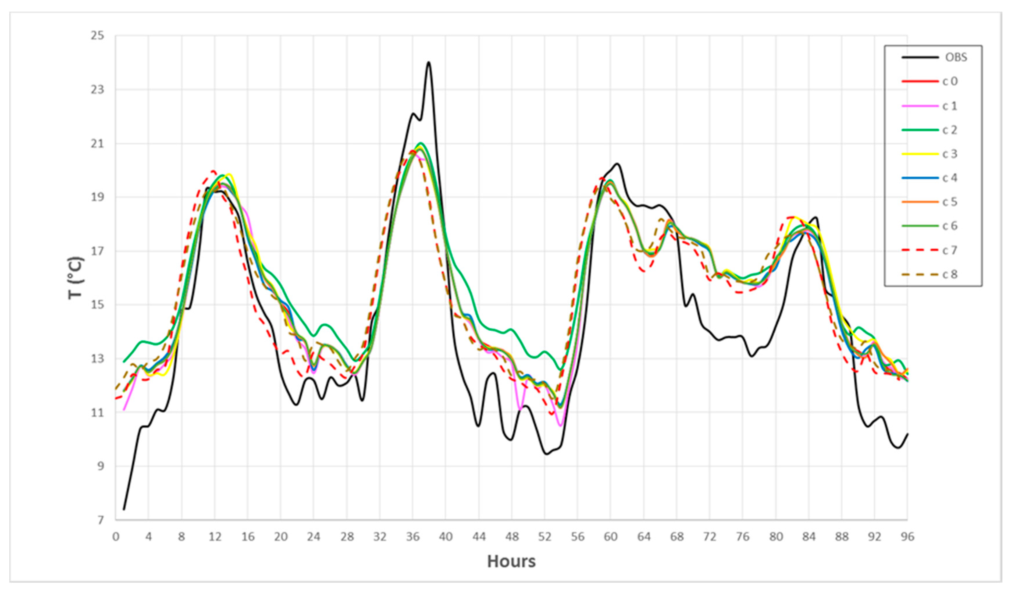
The first analysis was performed contemplating the hourly time series of T2m, comparing the data provided by the CIRA ground station with model data obtained with the different configurations, considering the nearest grid point to the CIRA site. Figure 2 shows the time series of T2m for observational and model data (reference configuration c0 and sensitivity configurations from c1 to c8) over a period of 96 h, from 01:00 3 November 2017 to 24:00 6 November 2017. In a similar way, Figure 3 shows the time series of T2m for observational data and model data (reference configuration c0 and sensitivity configurations from c9 to c18). For a better quantification of performances of sensitive runs, Table 3 shows the daily mean T2m values for each day considered in the 2017 and 2018 events for both observational and model data (all the configurations apply). The maximum deviation from the reference simulation with the initial condition ensemble (cP) is also shown. The last line contains the average cumulative errors with respect to observations. In a similar manner, Table 4 and Table 5 show, respectively, the daily maximum and minimum T2m values. It is evident that, with the c0 configuration, the maximum value of the first day is well reproduced, while it is underestimated in the other days. Mean and minimum values are overestimated in all days. A good improvement in the representation of maximum values is achieved with c7, which allows a null bias on 6 November 2017 and a bias reduction on 5 November 2017. The c15 allows a good improvement on 4–5 November 2017 and 19–20 November 2018, but conversely overestimates the maximum values on 3 and 6 November 2017. Good improvements are achieved also for the minimum values; in particular, c7 and c15 allow a better representation of the days of 2017 event, while c17 allows an improvement on 4 and 6 November 2017. Moreover, c1 performs better on 3 November 2017, while c14 and c16 perform better on 19 November 2018. Finally, for all the cases considered, the effects of internal variability (cP) are limited to small variations (about 1–2%).
In order to avoid the limitation of analysis related to a single spatial point, the effects of the sensitivity were investigated over a wider area, comparing model data with SCIA daily observational data. More specifically, six stations located in southern Lazio (namely Arpino, S. Elia Fiumerapido, S. Giorgio a Liri, Formia, Frosinone and Alvito) were considered. For each station, the nearest grid point was selected. Results are presented in terms of average values (average observational values and average model values for the different configurations). In detail, Table 6 shows the maximum daily values of T2m for 5 and 6 November 2017 and 19 and 20 November 2018. Similarly, Table 7 shows daily minimum values. The results highlight that the maximum values are always underestimated by c0, but improvements are achieved with several configurations, in particular with c17 for 5 November 2017, with c1 and c17 for 6 November 2017, and with c3 for 20 November 2018. Looking at the individual stations (value not shown in the tables), it shows that considerable improvements for the maximum temperature (bias reduction of 0.6 °C) are achieved in Arpino with c3 and c18, in S. Giorgio Liri with c7 and c17. Significant improvements for the minimum temperature (bias reduction of 0.5 °C) are achieved in Arpino with c7 and c17 and in Alvito with c15.
Even if observational data are not available over the whole domain, it is interesting to analyze how the sensitivity configurations modify the distribution of temperature with respect to the reference one. Figure 4 shows the T2m distribution related to 5 November 2017 at 6.00 (hour 54, corresponding to a minimum value) for the reference configuration c0 and the differences of distribution obtained with configurations that have been proven to produce better improvements (i.e., c1, c7, and c17) with respect to the reference one. The CIRA site is highlighted with a blue dot. From the data already discussed, it shows that c0 generally overestimates the minimum temperature. The maps of Figure 4 highlight that c7 and c17 provide lower values over the whole domain (generally reducing the bias), while with c1 benefits are confined to smaller areas, close to the CIRA site. Similarly, Figure 5 shows the T2m distribution related to 3 November 2017 (mean value) for c0, and the difference of distribution obtained with c7, c15, and c17 with respect to the reference one. As already said, c0 overestimates mean T2m of about 1.2 °C at the CIRA site, but the other three configurations are able to reduce significantly this bias. A reduction of temperature is observed over the northern Campania region (eastern part of the domain), while warmer temperatures are recorded in the northern part of the domain, over the sea and along the coastal area.

4.2. Analysis in Terms of Precipitation

The second analysis was performed considering daily precipitation values, comparing data provided by ANCE and SCIA with model data obtained with the different configurations. On 3–4 November 2017, observed precipitation values are almost zero everywhere, and these null values are well reproduced by all the model configurations (considering the nearest grid point). On 5–6 November 2017, and 20 November 2018 high precipitation was observed. Table 8 shows the daily precipitation values in these days, averaged over the whole network of 76 ANCE stations, for observational and model data (all the configurations). The maximum deviation from the reference simulation with the initial condition ensemble (cP) is also shown. These values reveal that c0 underestimates the observed value and that improvements are recorded with the configurations c3, c15, c16, and c18. These are all characterized by rlam_heat at minimum. For all the cases considered, the effects of internal variability (cP) are limited to small variations (about 2–3%). Then, more specifically, we analyzed the behavior of the model in selected stations at different altitudes, namely Benevento (135 m), Grazzanise (12 m), Montemarano (800 m), Giffoni (250 m). Table 9 and Table 10 show the observed and model values, respectively, for 6 November 2017 and 20 November 2018 for these stations, with the configurations (i.e., c3, c15, c16, c18) that have been proven to provide the best results. In Benevento and Grazzanise (low altitude sites) precipitation is largely underestimated by the reference configuration (more than 50%), but relevant improvements are achieved with c15 and c18. In Montemarano (high altitude) precipitation is slightly underestimated by c0, and quite improved by c18. In Giffoni (medium altitude), underestimation with c0 is more than 50%, but improvements are obtained with c16 and especially with c18 also in this case.
Table 11 shows the daily values of precipitation for 5–6 November 2017 and for 19–20 November 2018 (observational value and model data with the different configurations), averaged over the six stations taken from SCIA datasets (already considered for temperature analysis). Significant improvements are achieved with the same configurations already mentioned for ANCE data, namely c3, c15, c16, and c18. Looking at the individual stations (data not shown), it shows that (with the exception of Frosinone) precipitation is always underestimated with the reference configuration.
Even if gridded data over the whole area are not available, it is interesting to analyze how the sensitivity configurations modify the precipitation distribution with respect to the reference one. Figure 6 shows the precipitation distribution related to 6 November 2017 obtained with the reference configuration and the difference of distribution obtained with c3, c16, and c18 with respect to the reference one. These figures confirm that c3 and c18 are able to increase the average precipitation over wide areas of the domain. In particular, c3 and c18 (both characterized by rlam_heat at minimum) provide larger increases over low altitude areas, while enhancements are less relevant in high orography zones. Configuration c16 provides increases over southern Lazio (where the network of SCIA station is located, see also Table 11), while no (or small) variations are recorded over Campania. We also analyzed the maximum precipitation value over the entire simulated domain (values not shown), recording that it shows high variability with the configurations, ranging from minimum values (c5 and c7) to maximum values (c6 and c13).

4.3. Discussion

The previous analysis has revealed that variations in radqc_fact, fac_root_dp, and kexpdec produce very slight (or null) modifications of both T2m and precipitation values. Regarding the effects of variation of the other parameters, the following general considerations can be drawn on the basis of the results obtained:
A reduction of tkhmin causes a decrease of minimum and mean T2m. Stratification is made more stable, leading to decrease of night air temperature. On the other side, its increase causes a general increase of temperature, especially the minimum value (up to 1.5 °C). In fact, an increase of tkhmin implies that the turbulent kinetic energy is maintained in stable conditions, eliminating strong inversions [10]. A reduction of tkhmin does not cause variation in precipitation, while its increase causes a growth, since it increases the small convective cloudiness [24].
A reduction in rlam_heat causes a slight increase of T2m, while its increase does not modify the values of temperature with respect to c0. Generally, an increase of rlam_heat will increase the heat fluxes upward from the warm surface, leading to a larger heating of the lower atmosphere. Of course, this effect is more evident during the summer, while in the present test case the effects are less evident. Anyway, a not optimized setting of this parameter does not result in large temperature errors, since the soil moisture scheme implemented appropriately changes the soil moisture value. A reduction of rlam_heat causes the largest increase of precipitation, while its increase causes a reduction. In fact, the reduction of this parameter causes an increase of instability, leading to more precipitation. This effect is more evident for convective precipitation during summer.
An increase in v0snow causes a modest increase of precipitation. Variations have slight effects on the minimum value of T2m only, since this parameter is related to the temperature in an indirect way. In fact, the microphysical processes have an impact on the thermodynamics and the hydrological cycle via both direct and indirect feedback mechanisms.
A reduction in uc1 causes an increase of the maximum temperature and a reduction of the minimum, while an increase causes a slight reduction of the maximum temperature and a slight increase of the minimum. A reduction of uc1 increases the critical relative humidity level above the boundary layer, resulting in an increase of mid-level cloud formation, leading to an increase of maximum temperatures [18]. Variations in uc1 do not provide significant changes in precipitation.
The numerical results related to the four interaction simulations performed (defined in Table 2) allow drawing the following general considerations:
  • c15 provides an increase of the maximum temperature and a slight reduction of the minimum and mean T2m. It is also provides an increase of precipitation. This configuration is therefore able to improve the representation of both variables.
  • c16 provides slight achievements for precipitation representation.
  • c17 provides a slight increase of the maximum T2m and a slight reduction of the minimum and mean T2m, improving the simulation of temperature.
  • c18 is able to increase precipitation (improving its representation), along with an improvement of maximum temperature.
Analyzing the whole set of simulations performed, it shows that the best improvement for the representation of the mean T2m is achieved with uc1 at minimum (c7), even better when combined with rlam_heat at minimum (c15). Configuration c18 (rlam_heat at minimum and v0snow at maximum) provides a good representation of precipitation. In summary, even if the selection of the best configuration is beyond the purposes of the present work, as a result the configuration c15 is able to combine the best improvement for the maximum T2m, a slight improvement for the minimum T2m and the best representation for precipitation.

5. Conclusions

In this paper, the results of sensitivity experiments performed with the COSMO-LM model at very high resolution, over a domain located in southern Italy, are presented. The main aim of this work was to establish a hierarchy regarding the parameter sensitivity that could be useful in order to apply more advanced optimization techniques, such as the ones based on the application of meta-models. It was observed that some parameters have a strong impact and they could be a standalone source of further investigation, for a better understanding of the main physical processes in the atmosphere. Evaluation was performed in terms of temperature and precipitation against observational data provided by ground stations.
The present investigation revealed that over the area considered, the results of COSMO-LM in terms of temperature and precipitation show a great sensitivity to changes related to the physical parameterizations of soil and atmosphere. Effects of internal variability on the analysis presented were estimated, resulting in small variations. It was found that for the domain considered, better results in terms of temperature are obtained by choosing the minimum value of the parameter controlling the vertical variation of critical relative humidity for sub-grid cloud formation, even better when combined with the minimum value of the factor for laminar resistance for heat. This configuration allows a good improvement in terms of temperature bias (up to 0.5 °C) over this complex orographic area. Positive effects are observed also reducing the minimal diffusion coefficient for heat. Precipitation is generally underestimated by the reference configuration. These biases are partially due to shortcomings of the model in simulating some climate features of the area considered, along with deficiencies in the lateral boundary conditions and internal variability. Improvements in terms of precipitation for this area can be achieved by setting the factor for laminar resistance for heat at its minimum value. An increase in the value of factor for vertical velocity of snow also provides a positive effect on precipitation. Of course, further adjustments are needed in order to improve the spatial distribution of both temperature and precipitation. In particular, an approach based on an objective multi-variate calibration method built on a quadratic meta-model could be a useful tool in order to find a better combination of the values of the tuning parameters, even with respect to additional meteorological fields (e.g., cloud cover). The present results are valid for the considered mesh, while different (coarser) resolutions would require specific analyses. Anyway, the finding of the present work will be also applied to the configuration of ICON [35], a new model based on icosahedral grid that will replace COSMO in the next years.
That said, a detailed analysis of the capabilities of COSMO-LM in reproducing extreme events over this area must be performed considering even different periods and events, in order to have a statistical significance. This is suggested to be the topic of future work.

Author Contributions

Conceptualization, E.B.; formal analysis, A.V. and P.M.; investigation, E.B.; methodology, A.V.; validation, P.M.; writing—original draft, E.B. All authors have read and agreed to the published version of the manuscript.

Funding

This research received no external funding.

Acknowledgments

The authors would like to thank Jean Marie Bettems (MeteoSwiss) for providing the reference configuration and for the helpful discussions. The present study is performed within the framework of CALMO-MAX priority project of COSMO consortium. The work was performed as part of the employment of the authors, respectively, at CIRA and HNMS.

Conflicts of Interest

The authors declare no conflict of interest.

References

  1. Oreskes, N.; Shrader-Frechette, K.; Belitz, K. Verification, Validation, and Confirmation of Numerical Models in the Earth sciences. Science 1994, 263, 641–646. [Google Scholar] [CrossRef] [Green Version]
  2. Beven, K. Towards a coherent philosophy for modelling the environment. Proc. R. Soc. Lond. A 2002, 458, 2465–2484. [Google Scholar] [CrossRef] [Green Version]
  3. Jarvinen, H.; Laine, M.; Solonen, A.; Haario, H. Ensemble prediction and parameter estimation system: The concept. Q. J. R. Meteorol. Soc. 2011, 138, 281–288. [Google Scholar] [CrossRef]
  4. Ollinaho, P.; Laine, M.; Solonen, A.; Haario, H.; Jarvinen, H. NWP model forecast skill optimization via closure parameter variations. Q. J. R. Meteorol. Soc. 2013, 139, 1520–1532. [Google Scholar] [CrossRef]
  5. Ihshaish, H.; Cortes, A.; Senar, M. Genetic ensemble (GEnsemble) for meteorological prediction enhancement. In Proceedings of the 2011 Internacional Conference on Parallel and Distributed Processing Techniques and Applications (PDPTA2011), Las Vegas, NV, USA, 18–21 July 2011; Volume 1, pp. 404–410. [Google Scholar]
  6. Ihshaish, H.; Cortes, A.; Senar, M. Tuning G-ensemble to improve forecast skill in numerical weather prediction models. In Proceedings of the International Conference on Parallel and Distributed Processing Techniques and Applications PDPTA’12, WORLDCOMP’12, Las Vegas, NV, USA, 16–19 July 2012; pp. 869–875. [Google Scholar]
  7. Giorgi, F.; Mearns, L. Approaches to the simulation of regional climate change: A review. Rev. Geophys. 1991, 29, 191–216. [Google Scholar] [CrossRef]
  8. Bucchignani, E.; Cattaneo, L.; Panitz, H.J.; Mercogliano, P. Sensitivity analysis with the regional climate model COSMO-CLM over the CORDEX-MENA domain. Meteorol. Atmos. Phys. 2016, 128, 73–95. [Google Scholar] [CrossRef]
  9. Baldauf, M.; Seifert, A.; Förstner, J.; Majewski, D.; Raschendorfer, M.; Reinhart, T. Operational Convective-Scale Numerical Weather Prediction with the COSMO Model: Description and Sensitivities. Mon. Weather Rev. 2011, 139, 3887–3905. [Google Scholar] [CrossRef]
  10. Voudouri, A.; Khain, P.; Carmona, I.; Bellprat, O.; Grazzini, F.; Avgoustoglou, E.; Bettems, J.M.; Kaufmanne, P. Objective calibration of numerical weather prediction models. Atmos. Res. 2017, 190, 128–140. [Google Scholar] [CrossRef]
  11. Neelin, J.D.; Bracco, A.; Luo, H.; McWilliams, J.C.; Meyerson, J.E. Considerations for parameter optimization and sensitivity in climate models. Proc. Natl. Acad. Sci. USA 2010, 107, 21349–21354. [Google Scholar] [CrossRef] [Green Version]
  12. Bellprat, O.; Kotlarski, S.; Lüthi, D.; Schär, C. Objective calibration of regional climate models. J. Geophys. Res. 2012, 117, D23115. [Google Scholar] [CrossRef] [Green Version]
  13. Voudouri, A.; Khain, P.; Carmona, I.; Avgoustoglou, E.; Kaufmann, P.; Grazzini, F.; Bettems, J.M. Optimization of high resolution COSMO model performance over Switzerland and Northern Italy. Atmos. Res. 2018, 213, 70–85. [Google Scholar] [CrossRef]
  14. Duan, Q.; Di, Z.; Quan, J.; Wang, C.; Gong, W. Automatic Model Calibration: A New Way to Improve Numerical Weather Forecasting. BAMS 2017, 98, 959–970. [Google Scholar] [CrossRef]
  15. Avgoustoglou, E.; Voudouri, A.; Khain, P.; Grazzini, F.; Bettems, J.M. Design and Evaluation of Sensitivity Tests of COSMO model over the Mediterranean area. Perspect. Atmos. Sci. 2017, 1, 49–55. [Google Scholar]
  16. Milelli, M.; Bucchignani, E.; Mercogliano, P.; Garbero, V. Preliminary activity with COSMO-1 over Torino including TERRA-URB. COSMO Newsl. 2017, 17, 4–14. [Google Scholar]
  17. Steppeler, J.; Doms, G.; Schättler, U.; Bitzer, H.W.; Gassmann, A.; Damrath, U.; Gregoric, G. Meso-gamma scale forecasts using the nonhydrostatic model LM. Meteorol. Atmos. Phys. 2003, 82, 75–96. [Google Scholar] [CrossRef]
  18. Doms, G. A Description of the Nonhydrostatic Regional COSMO Model, Part I: Dynamics and Numerics; Technical Report; Deutscher Wetterdienst: Offenbach, Germany, 2002. [Google Scholar]
  19. Tiedtke, M. A comprehensive mass flux scheme for cumulus parameterization in large-scale models. Mon. Weather Rev. 1989, 117, 1779–1800. [Google Scholar] [CrossRef] [Green Version]
  20. Mellor, G.; Yamada, T. A hierarchy of turbulence closure models for planetary boundary layers. J. Atmos. Sci. 1974, 31, 1791–1806. [Google Scholar] [CrossRef] [Green Version]
  21. Hortal, M. The development and testing of a new two-time-level semi-Lagrangian scheme (SETTLS) in the ECMWF forecast model. Q. J. R. Meteorol. Soc. 2002, 128, 1671–1687. [Google Scholar] [CrossRef]
  22. Dierer, S.; Arpagaus, M.; Damrath, U.; Seifert, A.; Achimowicz, J.; Avgoustoglou, E.; Louka, P.; Fragkouli, V.; Dumitrache, R.; Grazzini, F.; et al. Final Report of the COSMO Priority Project “Tackle Deficiencies in Quantitative Precipitation Forecasts”; COSMO Consortium: Offenbach, Germany, 2007; Available online: http://www.cosmo-model.org/content/tasks/pastProjects/qpf/qpf_finalReport.pdf (accessed on 17 April 2020).
  23. Desiato, F.; Lena, F.; Toreti, A. SCIA: A system for a better knowledge of the Italian climate. Boll. Geofis. Teor. Appl. 2007, 48, 351–358. [Google Scholar]
  24. Voudouri, A.; Khain, P.; Carmona, I.; Avgoustoglou, E.; Bettems, J.M.; Grazzini, F.; Bellprat, O.; Kaufmann, P.; Bucchignani, E. Calibration of COSMO Model, Priority Project CALMO, Final Report; COSMO Technical Report; COSMO Consortium: Offenbach, Germany, 2017; p. 32. [Google Scholar]
  25. Doms, G.; Foerstner, J.; Heise, E.; Herzog, H.-J.; Mironov, D.; Raschendorfer, M.; Reinhardt, T.; Ritter, B.; Schrodin, R.; Schultz, J.-P.; et al. A Description of the Nonhydrostatic Regional COSMO Model. Part II: Physical Parameterization; COSMO Consortium: Offenbach, Germany, 2011; Available online: http://www.cosmo-model.org (accessed on 16 April 2020).
  26. Gebhardt, C.; Theis, S.E.; Paulat, M.; Ben Bouallègue, Z. Uncertainties in COSMO-DE precipitation forecasts introduced by model perturbations and variation of lateral boundaries. Atmos. Res. 2011, 100, 168–177. [Google Scholar] [CrossRef]
  27. Stull, R. An Introduction to Boundary Layer Meteorology; Kluwer Academic Publishers: Lordrecht, The Netherlands; Boston, MA, USA; London, UK, 1988. [Google Scholar]
  28. Cerenzia, I.; Tampieri, F.; Tesini, M.S. Diagnosis of turbulence schema in stable atmospheric conditions and sensitivity tests. COSMO Newsl. 2014, 14, 28–36. [Google Scholar]
  29. Raschendorfer, M. The New Turbulence Parameterization of LM, Quarterly Report of the. Operational NWP-Models of the DWD; Deutscher Wetterdienst: Offenbach, Germany, 1999; Volume 19, pp. 3–12. [Google Scholar]
  30. Stensrud, D.J. Paramerization Schemes: Keys to Understanding Numerical Weather Prediction Models; Cambridge University Press: New York, NY, USA, 2007; p. 459. [Google Scholar]
  31. Slingo, J.M. The Development and Verification of a Cloud Prediction Scheme for the Ecmwf Model. Q. J. R. Meteorol. Soc. 1987, 113, 899–927. [Google Scholar] [CrossRef]
  32. Decharme, B.; Douville, H.; Boone, A.; Habets, F.; Noilhan, J. Impact of an Exponential Profile of Saturated Hydraulic Conductivity within the ISBA LSM: Simulations over the Rhône Basin. J. Hydrometeorol. 2006, 7, 61–80. [Google Scholar] [CrossRef] [Green Version]
  33. Desborough, C.E. The Impact of Root Weighting on the Response of Transpiration to Moisture Stress in Land Surface Schemes. Mon. Weather Rev. 1997, 125, 1920–1930. [Google Scholar] [CrossRef]
  34. Bellprat, O. Parameter Uncertainty and Calibration of Regional Climate Models. Ph.D. Thesis, ETH Zurich, Zurich, Switzerland, 2013. [Google Scholar]
  35. Zängl, G.; Reinert, D.; Rípodas, P.; Baldauf, M. The ICON modelling framework of DWD and MPI-M: Description of the nonhydrostatic dynamical core. Q. J. R. Meteorol. Soc. 2015, 141, 563–579. [Google Scholar] [CrossRef]
Figure 1. The computational domain considered, including northern Campania and southern Lazio regions. The Italian Aerospace Research Center (CIRA) site is specified.
Atmosphere 11 00430 g001
Figure 2. Time series of T2m (°C) at the CIRA site for event 3–6 November 2017: observational and model data for reference configuration and sensitive configurations from c1 to c8.
Atmosphere 11 00430 g002
Figure 3. Time series of T2m (°C) at the CIRA site for event from 3 to 6 November 2017: observational and model data for reference configuration and sensitive configurations from c9 to c18.
Atmosphere 11 00430 g003
Figure 4. T2m distribution (°C) related to 5 November at 6.00 (hour 54) for configuration c0 (reference), and difference of distributions obtained with configurations c1, c7, and c17 compared to the reference one. The CIRA site is identified by a blue dot.
Atmosphere 11 00430 g004
Figure 5. T2m distribution (°C) related to 3 November (mean value) for configuration c0 (reference) and difference of distributions obtained with configurations c7, c15, and c17 compared to the reference one. The CIRA site is identified by a blue dot.
Atmosphere 11 00430 g005
Figure 6. Precipitation maps (mm) related to 6 November 2017 for configuration c0 (reference) and difference of distributions obtained with configurations c3, c16, and c18 compared to the reference one.
Atmosphere 11 00430 g006
Table 1. List of parameters considered for sensitive study and related values. Values of kexpdec varied between 0 and 1 in the sensitivity runs, even if the default value is 2.
ParameterizationNameMinimumDefaultMaximumDescription
Vertical turbulent diffusiontkhmin (m2/s)0.10.42Minimal diffusion coefficient for heat
Soil and vegetation processesrlam_heat (no units)0.112Factor for laminar resistance for heat
Microphysicsv0snow (no units)102030Factor for vertical velocity of snow
Radiationuc1 (no units)00.31Vertical variation of critical relative humidity for sub-grid cloud formation
Radiationradqc_fact (no units)0.30.60.9Fraction of cloud water and ice considered by the radiation scheme
Soil and vegetation processeskexpdec (m−1)021Factor for hydraulic conductivity
Soil and vegetation processesfac_rootdp (no units)0.511.5Modification factor for rootdp
Table 2. List of sensitivity runs and associated changes in the parameters with respect to c0.
Experiment NameModified Parameter Experiment NameModified Parameters
c0Defaultc10radfac (max)
c1tkhmin (min)c11fac_root_dp (min)
c2tkhmin (max)c12fac_root_dp (max)
c3rlam_heat (min)c13kexpdec at 0
c4rlam_heat (max)c14 kexpdec at 1
c5v0snow (min)c15rlam_heat (min), uc1 (min)
c6v0snow (max)c16rlam_heat (min), tkhmin (max)
c7uc1 (min)c17uc1 (min), v0snow (max)
c8uc1 (max) c18rlam_heat (min), v0snow (max)
c9Radfac (min)cPPerturbed initial conditions
Table 3. Daily mean two-meter temperature (T2m) values (°C) at the CIRA site for the days considered, for observational and model data (all configurations). Average cumulative errors with respect to observations. Maximum deviation (cP) from the reference simulation with the initial condition ensemble.
OBScPc0c1c2c3c4c5c6c7c8c9c10c11c12c13c14c15c16c17c18
3 November 201714.60.115.815.716.315.815.815.815.815.315.915.815.815.815.815.815.815.316.415.315.8
4 November 201715.30.2 15.715.716.315.815.715.715.715.715.815.815.815.715.715.815.815.716.215.615.8
5 November 201715.90.1 16.516.416.816.516.516.516.516.316.616.516.516.516.516.516.516.316.816.316.5
6 November 201713.60.2 15.115.115.415.415.015.215.115.015.215.115.115.115.115.115.115.215.714.915.3
19 November 201810.60.3 10.410.411.010.410.410.410.310.210.410.410.310.410.410.410.410.211.110.210.4
20 November 201814.90.1 16.416.416.616.416.416.416.316.116.416.416.416.416.416.416.416.116.616.116.4
Average error--0.80.81.20.90.80.80.80.60.90.80.80.80.80.80.80.61.30.50.8
Table 4. Daily maximum T2m values (°C) at the CIRA site for the days considered, for observational and model data (all configurations). Average cumulative errors with respect to observations. Maximum deviation (cP) from the reference simulation with the initial condition ensemble.
OBScPc0c1c2c3c4c5c6c7c8c9c10c11c12c13c14c15c16c17c18
3 November 201719.30.219.519.419.819.819.519.519.519.919.419.519.519.519.519.519.520.019.920.019.8
4 November 201724.00.320.820.521.020.820.720.720.720.720.620.620.720.820.820.720.720.921.020.720.9
5 November 201720.20.219.519.519.619.519.519.519.519.719.419.519.519.519.519.519.519.819.619.719.5
6 November 201718.20.217.817.717.918.217.617.817.818.217.717.817.817.817.817.817.818.618.318.218.3
19 November 201818.40.115.115.115.515.115.015.115.115.115.015.115.115.115.115.115.115.515.015.215.0
20 November 201820.50.219.119.119.319.119.119.119.119.119.019.119.119.119.119.119.119.319.019.219.1
Average error--−1.5−1.5−1.2−1.3−1.5−1.5−1.5−1.3−1.5−1.5−1.5−1.5−1.5−1.5−1.5−1.1−1.3−1.3−1.3
Table 5. Daily minimum T2m values (°C) at the CIRA site for the days considered, for observational and model data (all configurations). Average cumulative errors with respect to observations. Maximum deviation (cP) from the reference simulation with the initial condition ensemble.
OBScPc0c1c2c3c4c5c6c7c8c9c10c11c12c13c14c15c16c17c18
3 November 201710.50.112.512.313.512.412.612.512.512.212.612.512.512.512.512.512.511.613.312.212.4
4 November 201710.00.312.412.412.912.512.412.412.412.312.512.412.412.412.412.512.512.312.912.312.5
5 November 20179.50.211.210.512.611.211.311.211.210.911.511.211.211.211.211.211.211.012.611.011.2
6 November 20179.70.112.212.212.412.412.212.412.212.212.312.212.212.212.212.212.312.312.712.012.4
19 November 20188.10.37.37.38.07.47.37.37.37.27.57.37.37.37.37.37.77.37.77.37.4
20 November 201810.40.214.614.614.814.514.714.614.614.614.714.614.614.614.614.614.814.614.814.614.6
Average error--2.01.92.72.01.92.02.01.92.22.02.02.02.02.01.91.82.61.92.1
Table 6. Daily maximum T2m values (°C) averaged over the SCIA stations for the days considered, for observational and model data (all configurations). Maximum deviation (cP) from the reference simulation with the initial condition ensemble.
OBScPc0c1c2c3c4c5c6c7c8c9c10c11c12c13c14c15c16c17c18
5 November 201719.30.218.518.618.818.618.618.718.618.918.618.718.618.718.718.718.718.818.718.818.7
6 November 201718.50.117.818.218.018.117.917.917.917.917.917.917.917.917.917.817.918.018.118.218.0
19 November 201814.20.114.114.414.214.514.014.314.314.214.314.214.314.314.314.314.414.314.414.314.1
20 November 201818.40.416.116.116.216.616.016.116.116.016.116.216.216.116.116.116.216.116.216.016.1
Table 7. Daily minimum T2m values (°C) averaged over the SCIA stations for two days, for observational and model data (all configurations). Maximum deviation (cP) from the reference simulation with the initial condition ensemble.
OBScPc0c1c2c3c4c5c6c7c8c9c10c11c12c13c14c15c16c17c18
5 November 20177.80.29.39.19.49.39.29.29.29.09.39.29.29.29.29.29.29.19.59.19.3
6 November 20177.50.18.28.28.48.48.18.48.28.18.28.28.18.28.28.28.28.38.48.18.3
19 November 20182.70.36.56.56.76.76.26.76.56.06.56.56.46.56.56.56.56.66.86.06.5
20 November 20189.10.411.311.311.411.411.011.511.311.211.311.311.011.311.311.411.311.411.511.011.3
Table 8. Daily precipitation values (mm) averaged over the network of ANCE (Associazione Nazionale Costruttori Edili) stations, for observational and model data (all configurations). Maximum deviation (cP) from the reference simulation with the initial condition ensemble.
OBScPc0c1c2c3c4c5c6c7c8c9c10c11c12c13c14c15c16c17c18
5 November 201726.10.413.113.11316.912.413.413.113.213.013.113.113.113.113.113.017.114.117.117.8
6 November 201751.11.336.035.835.539.435.835.935.835.835.935.936.035.935.935.935.939.639.135.839.5
20 November 201834.70.522.222.122.030.321.622.522.622.522.521.022.222.122.222.222.229.225.224.230.3
Table 9. Daily precipitation values (mm) for 6 November 2019 for specific ANCE stations, for observational value and model data (selected configurations).
OBSc0c3c15c16c18
Benevento28.812.715.821.511.123.1
Grazzanise27.211.914.315.113.818.5
Montemarano40.625.621.023.523.630.1
Giffoni71.030.127.225.534.338.7
Table 10. Daily precipitation values (mm) for 20 November 2018 for specific ANCE stations, for observational value and model data (selected configurations).
OBSc0c3c15c16c18
Benevento18.913.215.616.511.017.5
Grazzanise25.812.016.720.220.427.2
Montemarano45.621.620.521.237.238.4
Giffoni5.00.00.32.02.51.3
Table 11. Daily precipitation values (mm) averaged over the network of SCIA stations, for observational and model data (all configurations). Maximum deviation (cP) from the reference simulation with the initial condition ensemble.
OBScPc0c1c2c3c4c5c6c7c8c9c10c11c12c13c14c15c16c17c18
5 November 201734.70.220.421.420.529.317.016.220.023.221.920.120.620.420.419.521.433.532.521.734.6
6 November 201721.90.39.49.79.414.29.27.610.18.59.59.89.59.49.49.69.213.114.69.414.9
19 November 201887.70.134.734.933.252.333.328.540.433.534.841.233.734.734.834.734.141.553.231.328.2
20 November 201831.90.323.224.622.528.323.023.227.524.223.623.822.923.023.122.923.028.429.023.527.2

