Article

Aridity Trends in Central America: A Spatial Correlation Analysis

1
Escuela de Estadística and Centro de Investigación en Matemática Pura y Aplicada, Universidad de Costa Rica, San José 11501, Costa Rica
2
Escuela de Física and Centro de Investigaciones Geofísicas, Universidad de Costa Rica, San José 11501, Costa Rica
3
Centro de Investigación en Ciencias del Mar y Limnología, Universidad de Costa Rica, San José 11501, Costa Rica
*
Author to whom correspondence should be addressed.
Atmosphere 2020, 11(4), 427; https://doi.org/10.3390/atmos11040427
Submission received: 23 February 2020 / Revised: 25 March 2020 / Accepted: 26 March 2020 / Published: 23 April 2020
(This article belongs to the Special Issue Central America and Caribbean Hydrometeorology and Hydroclimate)

Abstract

:
Trend analyses are common in several types of climate change studies. In many cases, finding evidence that the trends are different from zero in hydroclimate variables is of particular interest. However, when estimating the confidence interval of a set of hydroclimate stations or gridded data the spatial correlation between can affect the significance assessment using for example traditional non-parametric and parametric methods. For this reason, Monte Carlo simulations are needed in order to generate maps of corrected trend significance. In this article, we determined the significance of trends in aridity, modeled runoff using the Variable Infiltration Capacity Macroscale Hydrological model, Hagreaves potential evapotranspiration (PET) and near-surface temperature in Central America. Linear-regression models were fitted considering that the predictor variable is the time variable (years from 1970 to 1999) and predictand variable corresponds to each of the previously mentioned hydroclimate variables. In order to establish if the temporal trends were significantly different from zero, a Mann Kendall and a Monte Carlo test were used. The spatial correlation was calculated first to correct the variance of each trend. It was assumed in this case that the trends form a spatial stochastic process that can be modeled as such. Results show that the analysis considering the spatial correlation proposed here can be used for identifying those extreme trends. However, a set of variables with strong spatial correlation such as temperature can have robust and widespread significant trends assuming independence, but the vast majority of the stations can still fail the Monte Carlo test. We must be vigilant of the statistically robust changes in key primary parameters such as temperature and precipitation, which are the driving sources of hydrological alterations that may affect social and environmental systems in the future.
Dataset License: CC-BY-NC

Graphical Abstract

1. Introduction

Several types of climate change studies have found detectable trends in diverse hydroclimate variables, associated with anthropogenic climate signals that significantly stand out above the expected natural climate variability noise ([1,2,3,4]). In these examples, the trends of the first principal component (PC) of the hydroclimate variables (denoted the “fingerprint”) is compared to the statistical distribution of trends from the underlying natural climate variability represented in long pre-industrial “control” runs of coupled ocean-atmosphere general circulation climate models ([1,5,6]), or in some cases the distribution is obtained from proxy-data such as tree-rings ([4]).
In other studies not only the PC trend significance is of interest, but sometimes the spatial distribution of trends and their significance is of particular importance, as the location of significant changes is needed for determining the climate change impacts that may lead to adaptation and mitigation projects in the future. However, when estimating the significance of a set of hydroclimate stations (or gridded data) used in studies of detection of climate change signal or in common statistical trend analyses, the spatial correlation between the stations or grid points can affect the significance assessment ([6,7,8]). For this reason, Monte Carlo simulations are needed in order to generate maps of trend significance considering the effects of spatial correlation. In this article, we estimate the trends in aridity, runoff, potential evapotranspiration (PET) and near-surface temperature in Central America, and its variability, considering the effect of spatial correlation between the data points. It should be emphasized that the method proposed here results not in a correction of the significant trend maps considering spatial correlation, but instead the method highlights the locations of those extreme trend outliers. That is, for example, a temperature data set can present many stations with significant trends using traditional t-test statistics. The majority of these trends may be associated with a common domain-size signal (e.g., large-scale or synoptic) representing a main forcing mechanism such as global warming. Although the robustness of the warming signal could not questioned from the t-test, a few stations can have even more extreme warming trends; for example, associated with a combination of global warming and the location of heat islands in urban settings or drastic land use changes. Those extreme cases can be detected using the method presented here and they are associated with the spatial variability of the entire set, not only the individual t-tests at station scale.
Previous work ([9,10,11,12]) based on traditional non parametric and parametric tests showed widespread significant trends during the 20th and beginning of the 21st centuries in near-surface temperature in Central America and the Caribbean islands ([12,13]). These trends are positive in the vast majority of the cases, but in some locations are negative. Except for a few places, precipitation trends are non-significant, although this depends greatly on the database used in the assessment ([14,15]). Additionally, precipitation trends do not show a robust pattern over the isthmus as surface temperature do, because precipitation trends are constructed over multiscale processes ([16,17]). As a working hypothesis we argue that those stations showing a warming trend combined with a non-significant precipitation trend will result in increases of their aridity, as the demand of water from the atmosphere associated with increases in PET (due to warming) are not compensated by increases in the water supply from precipitation. Therefore, in a tropical region such as Central America, where the hydrology is not snow-dominated, one of the first indications of climate change associated with warming (if not offset by precipitation rises) is the increase in aridity and PET, along with reductions in runoff ([10,18]). We would like to test whether some of these hydrometeorological trends are significant and whether some of them are regionally significant.
The objectives of this work are: (1) Describe temporal trends for aridity, runoff, precipitation, PET and temperature, taking into account spatial correlation; (2) Highlight different conclusions depending whether or not the spatial correlation is taken into account; and (3) Conclude in terms of aridity for the Central American region if there is evidence of a regional trend or not in these variables for the 1970–1999 period.

2. Materials and Methods

A description of the data sources is given below:
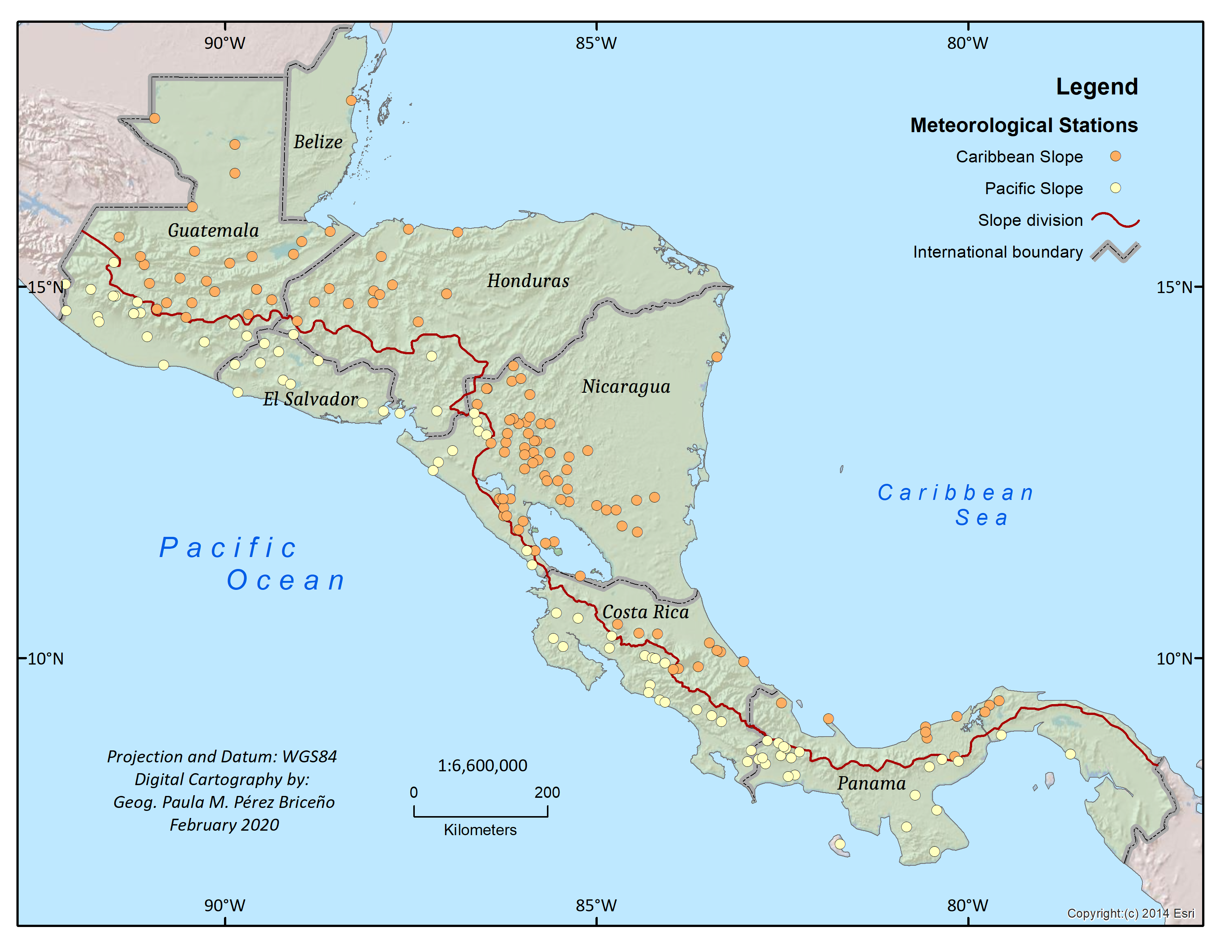
  • Precipitation: Monthly precipitation data for 199 stations in Central America from 1970 to 1999 were obtained from the NUMEROSA database of the Center for Geophysical Research (CIGEFI in Spanish) of the University of Costa Rica. The data were originally obtained at daily time scales from the national weather and hydrological services of Central America (Figure 1).
  • Temperature: Monthly near-surface temperature data were obtained from the database described in [9] (hereinafter referred as H2017). The H2017 is a gridded data set at 5 km × 5 km resolution over Central America, and the nearest grid points to the 199 precipitation station locations were selected for the analysis. The data were processed using a special weighted interpolation technique that considers seven kinds of weights: distance between the stations, elevation, cluster, vertical layer, topographic facet, coastal proximity and effective terrain. The interpolation is a variation of the Parameter-elevation Regressions on Independent Slopes (PRISM) method by [19,20,21]. The raw data for the interpolation was composed of temperature observations from NUMEROSA meteorological stations and a coarse gridded data set by [22]. For details, the reader can refer to [9], including the supplementary information. Monthly temperature data were used to derive maximum (Tmax) and minimum (Tmin) temperature daily values using the WeaGETS stochastic weather generator ([23]). Tmax and Tmin are necessary in the calculation of PET using the Hargreaves formula (see description below), and the daily temporal resolution is needed for the hydrological model runs (also described below). The parameters of WeaGETS were obtained from a set of 45 NUMEROSA Central America daily Tmax and Tmin meteorological stations depicted in Figure S1 of [9]. The parameters of the nearest station from this data set to each of the 199 H2017 locations were selected for WeaGETS simulations. Using WeaGETS, 300 years of daily Tmax and Tmin data were simulated at each of the H2017 locations to form a pool of candidate Tmax and Tmin daily data for desegregating the monthly H2017 average temperature data. The objective here is to produce an “acceptable” statistical pool of Tmin and Tmax values. Each month of H2017 data was compared to each candidate monthly average of simulated average of the Tmax and Tmin daily data, the closest simulated match was re-scaled to make it equal to the target H2017 month using an additive factor. The resulting factor was applied over all days of daily Tmax, Tmin and average temperature of the selected simulated month with the objective to constrain the monthly averages of the daily data to the monthly H2017 drifts. The procedure was repeated for each of the H2017 months from 1970 to 1999 and for all 199 locations.
  • Runoff: Total runoff (surface plus base flow) was obtained from modeling the precipitation and temperature data mentioned above, using the Variable Infiltration Capacity (VIC) macro scale hydrological model ([24]). VIC has been used in many climate variability and change applications at local and global domains ([2,18,25,26,27]). The daily precipitation and temperature data described before, along with wind-speed daily norms obtained from the National Center for Environmental Prediction and National Center for Atmospheric Research reanalysis ([28]) were used as meteorological forcing data for VIC simulations. At each of the 199 station locations, 1000 VIC simulations were obtained by varying the model’s parameters at random. The median of the 1000 simulations at each day composed the runoff daily time series at each of the 199 locations. The parameter ranges, as well as ancillary land surface information were obtained from [18]. The data were converted to annual averages.
  • PET: Monthly PET was obtained using the Hargreaves method ([29]) and the Tmax and Tmin temperature data, and radiation at the top of the atmosphere, which depends on julian day of the year and latitude.
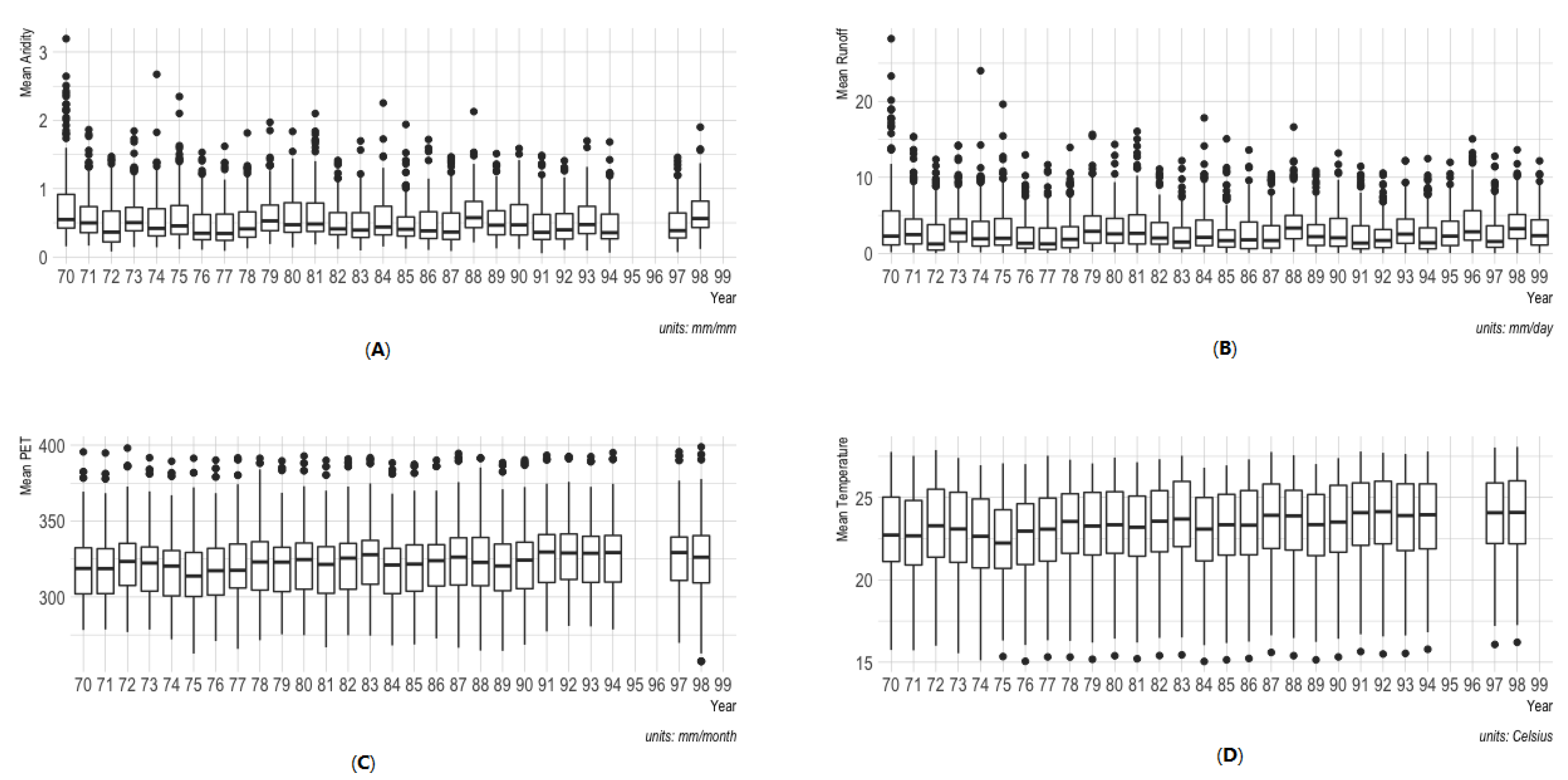
  • Aridity: An aridity index was computed as the annual average of the ratio of precipitation (representing water supply) over PET (representing water demand from the atmosphere). Smaller ratios are associated with higher aridity.
Visual inspection during quality control of the resulting daily data during some of the years showed significant outliers that were removed from the analysis. Not only were the extreme outliers (that were nonsensical like negative precipitation, or temperatures above 50 °C or below 0 °C in lowlands) removed, but also entire months of some of years were missing from the records and we decided to remove the entire year in those cases so that the data for that year was not biased to the months with available data. The are missing data in the runoff simulations as we run 1000 simulations of the hydrological model varying the parameters at random and sometimes the parameter combination produces non-feasible physical solutions and/or numerically unstable. This occurs very rarely, but they should be eliminated from the considered solutions.
The reason for using monthly data is that we were interested in annual trends (in temperature, PET, aridity and precipitation). In this particular paper we were not interested in trends in extreme indexes of these variables such as CLIMDEX (https://www.climdex.org/, as used in [11]). For each location, presented in Figure 1, the annual mean was calculated for each variable (Figure 2 and Figure A1). The reason for using annual trends is that aridity is a variable calculated at annual scales and we wanted to compare all measures of dryness and warming in the region. The main limitation with this approach is that we cannot detect trends in extreme events. With those annual data, linear slope estimates from least squares linear regression models were extracted, for which five different continuous response variables were used, showing respectively: runoff, aridity, precipitation, temperature, and PET centered in their mean per location. In all cases, years from 1970 to 1999 were used as predictors. A positive (negative) slope coefficient indicates an increasing (decreasing) linear trend and increasing (decreasing) quantity in each response variable over time (Figure 3). Each individual location is indexed as s and the data set comprise 199 stations per time point i. It is further assumed that each response variable, denoted as Y i ( s ) , is linearly related to the year covariate, denoted as X i , and that the residuals ϵ i ( s ) are distributed as independently and identically as N ( 0 , σ 2 ) . A linear regression model with one predictor variable can be expressed with the following equation: Y i ( s ) = β ( s ) X i + ϵ i ( s ) , given that the response variable Y i is centered in zero. The parameter of interest in the model is β ( s ) , the slope coefficient representing the linear trend over time, which is extracted from the model summary for each location.
As [8] pointed out, when working with hydroclimate variables, testing for trend at each site separately, and ignoring of spatial correlation between variables from the different sites, results in having too many trends that are considered to be significant when they are not. Hence, we compare the results of a Mann–Kendall Trend test used in [2] with a traditional t-test and with an interval constructed under the null hypothesis of no trend, and assuming spatial correlation. For that, since we are interested in the estimation of the parameters that describe the spatial relationship, empirical variograms are used to explore the spatial correlation between the trends at each site.
The calculated linear trends can be seen as realizations of a stationary spatial stochastic process, denoted by Z ( s ) = β + ϵ ( s ) for location s, with mean trend β , i.e., the average taken over all of the stations available. The interest in this case is modeling the spatial dependence of Z ( s ) , for which the empirical variogram γ ( h ) is calculated by γ ( h ) = 1 2 V a r { Z ( s ) Z ( s h ) } where h is a measure of distance between two locations [30]. The observed process can be modeled with different theoretical structures, among them the Gaussian model with nugget, represented by:
γ ( h ) = τ 2 + σ 2 ( 1 exp ( h 2 / a 2 ) )
where τ 2 (nugget parameter) represents the uncertainty or measurement error in the linear trend, and  σ 2 its variability. Here, exp ( h / a ) is the correlation function between two sites separated by h distance and where a represents the maximum distance (range) for which the spatial correlation is important. Therefore, the parameters of interest in this case are τ 2 , σ 2 , and a, although in some cases the nugget can be set to zero.
With the parameters estimated, each of the cells ( s i , s j ) of the variance-covariance matrix of the errors Σ ( s i , s j ) , can be calculated according to the respective distance h between each pair of locations ( s i , s j ) , using the formula: Σ ( h ) = I i = j ( h ) τ ^ 2 + σ ^ 2 ( 1 exp ( h 2 / a ^ 2 ) ) , where I i = j ( h ) is an indicator function meaning that the nugget parameter is only added to the diagonal cells. Then, a confidence interval can be calculated using parametric bootstrap for all trends, as recommended in [31]. Equivalently, what we propose is to estimate Σ ( s i , s j ) for all i and j locations, to then use it to generate samples of a multivariate normal centered in zero, as the distribution of Z(s) when its mean is zero. The distribution of the null hypothesis, i.e., assuming that the empirical distribution of M = 5000 samples of trends is centered in zero, is then compared with the observed value of the trend, to confirm if this value is or not included between the 0.025 th and 0.975 th quantiles of the null hypothesis empirical distribution.
Statistical analysis were performed using the computing environment R [32]. The code and data to perform each of the analysis mentioned in this paper are available for download in https://malfaro2.github.io/Hidalgo_CIGEFI2/. Data formatting and figures were prepared using the collection of R packages Tidyverse [33].

3. Results

Five hydroclimate variables: aridity, runoff, precipitation, temperature and PET were summarized, centered and regressed against years in each of the 199 locations. Animations for the spatial temporal variables are available at https://malfaro2.github.io/Hidalgo_CIGEFI2/. Temperature, PET (function of temperature) and aridity (function of both PET and precipitation), had 1995, 1996 and 1999 as missing values, since they presented important data quality issues in the daily records. Likewise, precipitation presented quality issues values during 1995 and 1999 for some locations and the data for those years was not used. A description of the variables statistics can be found in Table 1, Figure 1 and Figure A1.
The linear trends were calculated in each location, having a total of 199 trends per variable. Figure 3 present the scale and values for each of the trends. Although there are points with values that seem to be significantly different from zero, the question of interest in this case is to characterize the spatial dependence and see if the extreme trends are highlighted after taking it into account.

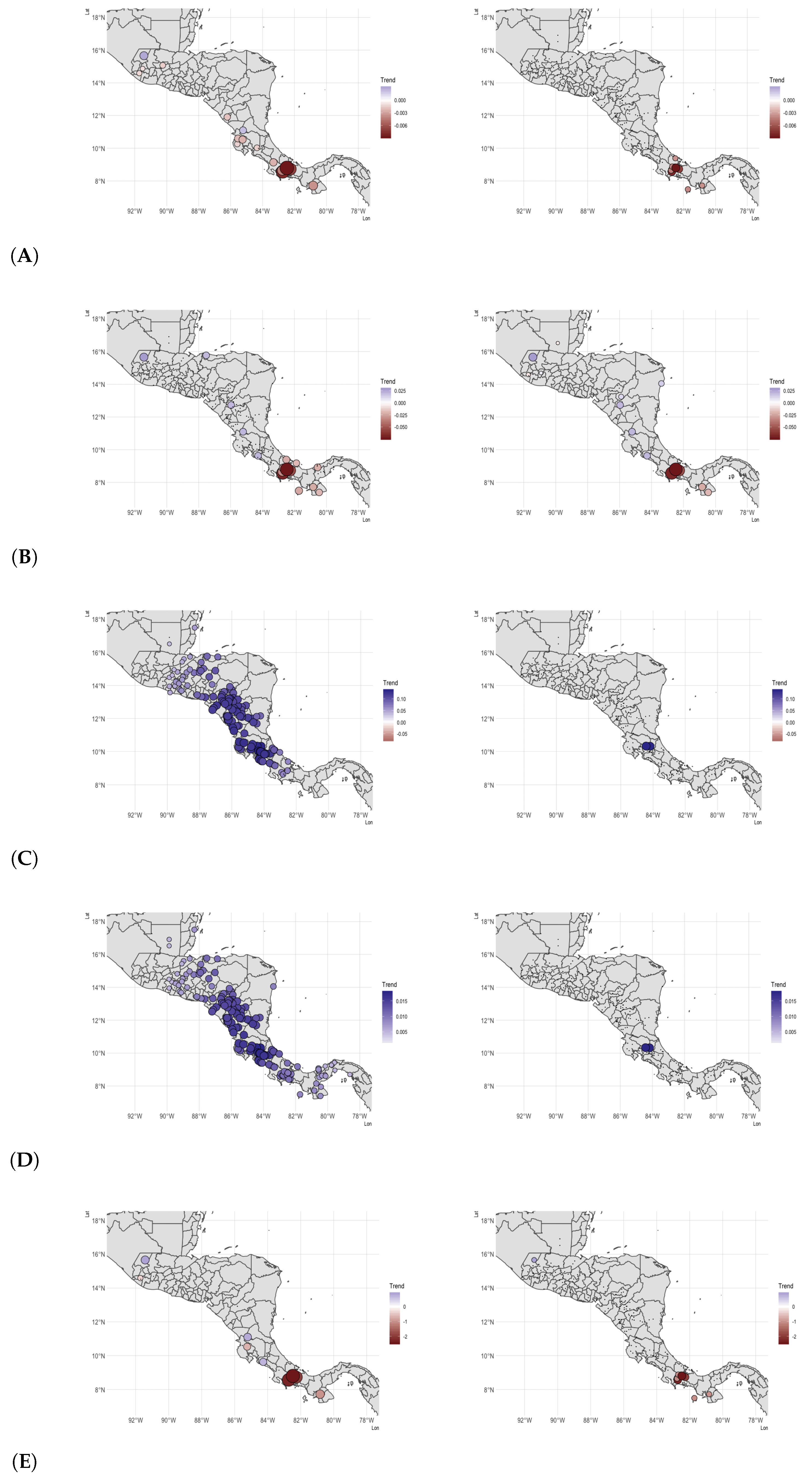
3.1. Spatial Modeling

In order to characterize the spatial dependence, an empirical variogram modeling was performed for each variable separately, but first, a randomized test was perform to test for spatial dependence. Each sample variogram was compared to 100 variograms for randomly re-allocated data, as recommended by [30] to detect spatial structures. The results for the trend of variable PET are presented in Figure 4, very similar results were obtained with the other four variables, which means that all empirical variograms have evidence to reject the null hypothesis of absence of spatial correlation. Next, the empirical variograms were modeled with several options, and in all cases a Gaussian model was the most adequate. The results are presented in Table 2. The ranges are given in Euclidean distances between the location coordinates, and the variance parameters (nugget and psill) are given according to the variable scale.
While the empirical variogram fitting solution is not unique in this case, the minimization of the sum of squares of error is used to choose the best option. Weighted R 2 is reported in Table 2 for reference, although the sum of squares is not the ideal goodness of fit measure for these nonlinear fittings.
The dependency can be described as strong for locations close together in cases where the range is small, and the psill is very big compared to the nugget, such as with PET and temperature. Nevertheless, for locations that are farther away than the range, the spatial dependency fades away. For runoff and precipitation, the ranges are rather big (such as 10.00 degrees), which means that locations that are far apart still can have a strong dependence, but note that in these two cases the difference between the nugget and the psill is of one order of magnitude, which compared to the case of PET and temperature is a small difference, and therefore a smaller spatial dependence.
Temperature is originally a product of a (sophisticated) interpolation model, and as such these spatial characteristics are intrinsically present in its parameters ([9]). In the same manner PET is a function of temperature, and present similar defining characteristics.

3.2. Temporal Trends Confidence Intervals

Two separate analyses were performed using the trend data for each variable. The first one was constructing the confidence intervals assuming that all the locations were independent, for comparison. The second one was using the empirical variogram modeling to calculate Σ for each variable, and then, simulating an empirical distribution assuming that it is centered in zero. With Monte Carlo runs, an empirical distribution for the null hypothesis is constructed and then each calculated trend is compared with the 95 % confidence interval.
Figure 5 and Figure 6 show the results for each variable. The confidence intervals constructed assuming independence are presented in Figure 5, and the maps with the significant trends assuming each of the locations represent an independent random sample (left panel), and the maps with the same trends, but now assuming that they are spatially correlated according to the models specified in Section 3.1 are presented (right panel) in Figure 6.

4. Discussion

In general, Figure 5 and Figure 6 show that, without considering spatial correlation, there are widespread significant increasing trends in PET and temperature during the 1970–1999 period. As showed previously in [9,11,12,13], temperature warming trends are the most robust, in terms of sign, of the analysis in the present work. In the case of aridity and runoff only selected locations (most of them in Costa Rica and Nicaragua) show significant trends, and in general are negative, suggesting a consistency with our working hypothesis and with [10,18]. Precipitation, only show a few significant trends, and most of them toward reductions.
When considering the spatial correlation of the data, only those extreme trends stand out from the distribution (Figure 5 and right panel of Figure 6). At this point, it is important to mention that by construction, the method presented here result in quantiles in which most of the trends are inside the 95 % bounds, assuming that the mean of the distribution is zero. For example, in the case of temperature, a large spatial correlation which could be the product of the interpolation method used and the relatively large (with respect to the study domain) controlling climate mechanisms would result in a large standard deviation that would include most of the observed trends within the 95 % bounds. In this sense, the method tends to classify as significant only the very extreme trends. The utility of this, is to identify, which trends are outside the range related to main domain size forcing climatic mechanism. In the particular case of temperature, it seems that the northern region of Costa Rica stands out as having significant trends that are even stronger than the main widespread trends presumably associated with global warming. In the case of precipitation, some precipitation reductions in Panama seem to be extremely significant, driving extreme trends in aridity and runoff.
There are important differences between the trend significance when assuming independence, compared to those obtained using a spatial dependence correction in all variables, as pointed out by [8,31]. Differences are due to the clear spatial dependence that can be noted in Figure 3 and Figure 5. This dependence was modeled using empirical variogram modeling, and the estimated Σ was used to generate the Monte Carlo samples. The nugget to psill ratio presented in Table 2 gives clear evidence of a strong spatial dependence for PET and temperature, and a smaller dependence for aridity, precipitation and runoff.

5. Conclusions

From the analysis of the uncorrected trends it is evident that widespread warming during the 1970–1999 period is still not sufficient to drive equally widespread significant aridity changes as stated in our working hypothesis. This is because the majority of the aridity trends were not significant. As temperature increased (associated with water demand) while precipitation remained the same (associated with water supply), we would expect for aridity to increase, but the trends are still non-significant. However, it is worrisome that aridity is increasing and runoff is decreasing in some locations of Costa Rica and Nicaragua. For example, one of the aridity increases is located in the headwaters of the Tempisque catchment in Costa Rica. The Tempisque catchment is the largest in the country and an important source of irrigation water in the Costa Rican North Pacific ([34,35]), a relatively drier zone which is part of the Central American Dry Corridor ([10,36,37,38]). Decreasing precipitation trends have also been reported in the Tempisque headwaters by [39] using another dataset. Future research should focus on determining if recent and projected future warming can bring higher aridity to the region and jeopardize water resources, especially in Nicaragua and Costa Rica, where many stations already showed significant warming and some locations reported significant decreasing runoff trends. Panama showed some locations with increasing aridity trends and reducing runoff trends, but they seem to be more related to significant precipitation reductions than to warming trends.
Accounting for spatial correlation in the method presented here results in identification of the locations where trends are the most extreme. Although the approach followed here does not result in a correction method for spatial correlation in similar fashion as [7], it can be used to suggest that, in terms of temperature and PET, there are coherent significant increasing trends that are bounded within a regional signal. Other variables show less robust trends in the sense that have negative and positive trends that are outliers, and not only positive as PET and temperature.
Climate change would bring hydrological alterations in the region associated with warmer temperature, increased aridity, reduced runoff and drier soils. The continuing monitoring of these variables is important, as the first indications of these changes are beginning to emerge. We must be vigilant of the statistically robust changes in key primary parameters such as temperature and precipitation, which are the driving sources of hydrological alterations that may affect social ([40]) and environmental ([41]) systems in the future.

Author Contributions

Conceptualization, H.G.H., E.J.A. and M.A.-C.; methodology, H.G.H., E.J.A., M.A.-C.; software, M.A.-C.; validation, H.G.H., E.J.A.; formal analysis, H.G.H., M.A.-C.; investigation, H.G.H., E.J.A. and M.A.-C.; resources, H.G.H., E.J.A.; data curation, M.A.-C.; writing–original draft preparation, H.G.H., E.J.A. and M.A.-C.; writing–review and editing, H.G.H., E.J.A. and M.A.-C.; visualization, M.A.-C.; supervision, H.G.H., E.J.A.; project administration, H.G.H., E.J.A.; funding acquisition, H.G.H., E.J.A. All authors have read and agreed to the published version of the manuscript.

Funding

The authors wish to acknowledge the funding of this research through the following Vicerrectoría de Investigación, Universidad de Costa Rica grants: V.I. 805-B0-810, B8-766 (Redes Temáticas), B9-454 (Grupos), EC-497 (VarClim) and C0-471 (Fondo de Estímulo).

Acknowledgments

To the UCR Schools of Physics and Statistics for giving us the research time to develop this study. To the UCR research centers CIGEFI and CIMPA for their logistic support during the data compilation and analysis. To the Central American NW & HSs for providing the data used in this work. To Paula Marcela Pérez Briceño for her assistance with Figure 1. The authors would like to recognize the help of Pablo Imbach in the construction of the NUMEROSA database. We thank students Josín Madrigal and Andrés Jiménez, who helped with data processing.

Conflicts of Interest

The authors declare no conflict of interest.

Abbreviations

The following abbreviations are used in this manuscript:
PETPotential Evapotranspiration
H2017Monthly temperature database from [9]
TmaxNear-surface maximum air temperature
TminNear-surface minimum air temperature
VICVariable Infiltration Capacity macroscale hydrological model
MADMean absolute deviations

Appendix A

Figure A1. Boxplot describing data from 1970–1999 in the Central American Region, for each of the following variables: (A) Aridity. (B) Runoff. (C) PET. (D) Temperature.
Atmosphere 11 00427 g0a1

References

  1. Barnett, T.P.; Pierce, D.W.; Hidalgo, H.G.; Bonfils, C.; Santer, B.D.; Das, T.; Bala, G.; Wood, A.W.; Nozawa, T.; Mirin, A.A.; et al. Human-Induced Changes in the Hydrology of the Western United States. Science 2008, 319, 1080–1083. [Google Scholar] [CrossRef] [Green Version]
  2. Hidalgo, H.G.; Das, T.; Dettinger, M.D.; Cayan, D.R.; Pierce, D.W.; Barnett, T.P.; Bala, G.; Mirin, A.; Wood, A.W.; Bonfils, C.; et al. Detection and Attribution of Streamflow Timing Changes to Climate Change in the Western United States. J. Clim. 2009, 22, 3838–3855. [Google Scholar] [CrossRef]
  3. IPCC. Climate Change 2013—The Physical Science Basis; Cambridge University Press: Cambridge, UK, 2009. [Google Scholar] [CrossRef] [Green Version]
  4. Marvel, K.; Cook, B.I.; Bonfils, C.J.W.; Durack, P.J.; Smerdon, J.E.; Williams, A.P. Twentieth-century hydroclimate changes consistent with human influence. Nature 2019, 569, 59–65. [Google Scholar] [CrossRef] [PubMed]
  5. Pierce, D.W.; Barnett, T.P.; Hidalgo, H.G.; Das, T.; Bonfils, C.; Santer, B.D.; Bala, G.; Dettinger, M.D.; Cayan, D.R.; Mirin, A.; et al. Attribution of Declining Western U.S. Snowpack to Human Effects. J. Clim. 2008, 21, 6425–6444. [Google Scholar] [CrossRef] [Green Version]
  6. Das, T.; Hidalgo, H.G.; Pierce, D.W.; Barnett, T.P.; Dettinger, M.D.; Cayan, D.R.; Bonfils, C.; Bala, G.; Mirin, A. Structure and Detectability of Trends in Hydrological Measures over the Western United States. J. Hydrometeorol. 2009, 10, 871–892. [Google Scholar] [CrossRef] [Green Version]
  7. Livezey, R.E.; Chen, W.Y. Statistical Field Significance and its Determination by Monte Carlo Techniques. Mon. Weather Rev. 1983, 111, 46–59. [Google Scholar] [CrossRef] [Green Version]
  8. Buarque, D.C.; Clarke, R.T.; Mendes, C.A.B. Spatial correlation in precipitation trends in the Brazilian Amazon. J. Geophys. Res. 2010, 115. [Google Scholar] [CrossRef]
  9. Hidalgo, H.G.; Alfaro, E.J.; Quesada-Montano, B. Observed (1970–1999) climate variability in Central America using a high-resolution meteorological dataset with implication to climate change studies. Clim. Chang. 2017, 141, 13–28. [Google Scholar] [CrossRef] [Green Version]
  10. Hidalgo, H.G.; Alfaro, E.J.; Amador, J.A.; Bastidas, Á. Precursors of quasi-decadal dry-spells in the Central America Dry Corridor. Clim. Dyn. 2019, 53, 1307–1322. [Google Scholar] [CrossRef]
  11. Aguilar, E.; Peterson, T.C.; Obando, P.R.; Frutos, R.; Retana, J.A.; Solera, M.; Soley, J.; García, I.G.; Araujo, R.M.; Santos, A.R.; et al. Changes in precipitation and temperature extremes in Central America and northern South America, 1961–2003. J. Geophys. Res. Atmos. 2005, 110. [Google Scholar] [CrossRef]
  12. Jones, P.D.; Harpham, C.; Harris, I.; Goodess, C.M.; Burton, A.; Centella-Artola, A.; Taylor, M.A.; Bezanilla-Morlot, A.; Campbell, J.D.; Stephenson, T.S.; et al. Long-term trends in precipitation and temperature across the Caribbean. Int. J. Climatol. 2016, 36, 3314–3333. [Google Scholar] [CrossRef] [Green Version]
  13. Stephenson, T.S.; Vincent, L.A.; Allen, T.; Van Meerbeeck, C.J.; McLean, N.; Peterson, T.C.; Taylor, M.A.; Aaron-Morrison, A.P.; Auguste, T.; Bernard, D.; et al. Changes in extreme temperature and precipitation in the Caribbean region, 1961–2010. Int. J. Climatol. 2014, 34, 2957–2971. [Google Scholar] [CrossRef]
  14. Hannah, L.; Donatti, C.I.; Harvey, C.A.; Alfaro, E.; Rodriguez, D.A.; Bouroncle, C.; Castellanos, E.; Diaz, F.; Fung, E.; Hidalgo, H.G.; et al. Regional modeling of climate change impacts on smallholder agriculture and ecosystems in Central America. Clim. Chang. 2017, 141, 29–45. [Google Scholar] [CrossRef] [Green Version]
  15. Cavazos, T.; Luna-Niño, R.; Cerezo-Mota, R.; Fuentes-Franco, R.; Méndez, M.; Martínez, L.F.P.; Valenzuela, E. Climatic trends and regional climate models intercomparison over the CORDEX-CAM (Central America, Caribbean, and Mexico) domain. Int. J. Climatol. 2019. [Google Scholar] [CrossRef]
  16. Hidalgo-León, H.G.; Herrero-Madriz, C.; Alfaro-Martínez, E.J.; Muñoz, A.G.; Mora-Sandí, N.P.; Mora-Alvarado, D.A.; Chacón-Salazar, V.H. Urban Waters in Costa Rica. In Urban Water Challenges in the Americas. A Perspective from the Academies of Sciences; Vammen, K., de la Cruz-Molina, A., Eds.; The Inter-American Network of Academies of Sciences (IANAS): Distrito Federal, Mexico, 2015; pp. 202–225. [Google Scholar]
  17. Anderson, T.G.; Anchukaitis, K.J.; Pons, D.; Taylor, M. Multiscale trends and precipitation extremes in the Central American Midsummer Drought. Environ. Res. Lett. 2019, 14, 124016. [Google Scholar] [CrossRef]
  18. Hidalgo, H.G.; Amador, J.A.; Alfaro, E.J.; Quesada, B. Hydrological climate change projections for Central America. J. Hydrol. 2013, 495, 94–112. [Google Scholar] [CrossRef]
  19. Daly, C.; Neilson, R.P.; Phillips, D.L. A Statistical-Topographic Model for Mapping Climatological Precipitation over Mountainous Terrain. J. Appl. Meteorol. 1994, 33, 140–158. [Google Scholar] [CrossRef] [Green Version]
  20. Daly, C.; Gibson, W.P.; Taylor, G.H.; Johnson, G.L.; Pasteris, P. A knowledge-based approach to the statistical mapping of climate. Clim. Res. 2002, 22, 99–113. [Google Scholar] [CrossRef] [Green Version]
  21. Daly, C.; Halbleib, M.; Smith, J.I.; Gibson, W.P.; Doggett, M.K.; Taylor, G.H.; Curtis, J.; Pasteris, P.P. Physiographically sensitive mapping of climatological temperature and precipitation across the conterminous United States. Int. J. Climatol. 2008, 28, 2031–2064. [Google Scholar] [CrossRef]
  22. Maurer, E.P.; Adam, J.C.; Wood, A.W. Climate model based consensus on the hydrologic impacts of climate change to the Rio Lempa basin of Central America. Hydrol. Earth Syst. Sci. 2009, 13, 183–194. [Google Scholar] [CrossRef] [Green Version]
  23. Chen, J. Stochastic Weather Generator (WeaGETS), MATLAB Central File Exchange. 2020. Available online: https://www.mathworks.com/matlabcentral/fileexchange/29136-stochastic-weather-generator-weagets (accessed on 8 January 2020).
  24. Liang, X.; Lettenmaier, D.P.; Wood, E.F.; Burges, S.J. A simple hydrologically based model of land surface water and energy fluxes for general circulation models. J. Geophys. Res. 1994, 99, 14415–14428. [Google Scholar] [CrossRef]
  25. Lin, P.; Pan, M.; Beck, H.E.; Yang, Y.; Yamazaki, D.; Frasson, R.; David, C.H.; Durand, M.; Pavelsky, T.M.; Allen, G.H.; et al. Global Reconstruction of Naturalized River Flows at 2.94 Million Reaches. Water Resour. Res. 2019, 55, 6499–6516. [Google Scholar] [CrossRef] [PubMed] [Green Version]
  26. Zhu, Y.; Liu, Y.; Wang, W.; Singh, V.P.; Ma, X.; Yu, Z. Three dimensional characterization of meteorological and hydrological droughts and their probabilistic links. J. Hydrol. 2019, 578. [Google Scholar] [CrossRef]
  27. Rakovec, O.; Mizukami, N.; Kumar, R.; Newman, A.J.; Thober, S.; Wood, A.W.; Clark, M.P.; Samaniego, L. Diagnostic Evaluation of Large-Domain Hydrologic Models Calibrated Across the Contiguous United States. J. Geophys. Res. Atmos. 2019. [Google Scholar] [CrossRef] [Green Version]
  28. Kalnay, E.; Kanamitsu, M.; Kistler, R.; Collins, W.; Deaven, D.; Gandin, L.; Iredell, M.; Saha, S.; White, G.; Woollen, J.; et al. The NCEP/NCAR 40-Year Reanalysis Project. Bull. Am. Meteorol. Soc. 1996, 77, 437–472. [Google Scholar] [CrossRef] [Green Version]
  29. Hargreaves, G.H. Moisture Availability and Crop Production. Trans. Am. Soc. Agric. Eng. 1975, 18, 980–984. [Google Scholar] [CrossRef]
  30. Bivand, R.S.; Pebesma, E.J.; Gómez-Rubio, V. Applied Spatial Data Analysis with R; Springer: New York, NY, USA, 2008. [Google Scholar] [CrossRef]
  31. Azam, M.; Maeng, S.; Kim, H.; Lee, S.; Lee, J. Spatial and Temporal Trend Analysis of Precipitation and Drought in South Korea. Water 2018, 10, 765. [Google Scholar] [CrossRef] [Green Version]
  32. R Core Team. R: A Language and Environment for Statistical Computing; R Foundation for Statistical Computing: Vienna, Austria, 2018. [Google Scholar]
  33. Wickham, H. Welcome to the tidyverse. J. Open Source Softw. 2019, 4, 1686. [Google Scholar] [CrossRef]
  34. Alfaro, E.J. Caracterización del “veranillo” en dos cuencas de la vertiente del Pacífico de Costa Rica, América Central. Rev. De Biol. Trop. 2014, 62, 1–15. [Google Scholar] [CrossRef] [Green Version]
  35. Alfaro, E.J.; Hidalgo, H.G. Propuesta metodológica para la predicción climática estacional del veranillo en la cuenca del río Tempisque, Costa Rica, América Central. Tópicos Meteorológicos Y Ocean. 2017, 16, 62–74. [Google Scholar]
  36. Gotlieb, Y.; Pérez-Briceño, P.M.; Hidalgo, H.G.; Alfaro, E.J. The Central American Dry Corridor: A consensus statement and its background. Rev. Yu’am 2019, 3, 42–51. [Google Scholar]
  37. Quesada-Hernández, L.E.; Calvo-Solano, O.D.; Hidalgo, H.G.; Pérez-Briceño, P.M.; Alfaro, E.J. Dynamical delimitation of the Central American Dry Corridor (CADC) using drought indices and aridity values. Prog. Phys. Geogr. Earth Environ. 2019, 43, 627–642. [Google Scholar] [CrossRef]
  38. Quesada-Hernández, L.E.; Hidalgo, H.; Alfaro, E. Asociación entre algunos índices de sequía e impactos socio-productivos en el Pacífico Norte de Costa Rica. Rev. De Cienc. Ambient. 2020, 54, 16–32. [Google Scholar] [CrossRef] [Green Version]
  39. Quesada-Hernández, L.E. Respuesta de la hidrología superficial de la cuenca del Río Tempisque a la variabilidad climática y cambio de cobertura de la tierra. Master’s Thesis, Universidad de Costa Rica, San Pedro, San José, Costa Rica, 2019. (In Spanish). [Google Scholar]
  40. Hidalgo, H.G.; Alfaro, E.J. Some physical and socio-economic aspects of climate change in Central America. Prog. Phys. Geogr. Earth Environ. 2012, 36, 379–399. [Google Scholar] [CrossRef]
  41. Moreno, M.L.; Hidalgo, H.G.; Alfaro, E.J. Cambio climático y su efecto sobre los servicios ecosistémicos en dos parques nacionales de Costa Rica, América Central. Rev. Iberoam. De Econ. Ecológica 2019, 30, 16–38. [Google Scholar]
Figure 1. Location for 199 meteorological stations in the Central American Region. Yellow and orange dots are gauge stations located in the Pacific and Caribbean slope, respectively.
Atmosphere 11 00427 g001
Figure 2. Boxplot for annual Precipitation (mm/month) means in the Central American Region 1970–1999.
Atmosphere 11 00427 g002
Figure 3. Trends for (A) Precipitation, (B) Runoff, (C) Aridity, (D) PET and (E) Temperature for 199 meteorological stations in the Central American Region. The dashed black vertical line corresponds to zero trend or no change over the years 1970–1999. Outliers were detected using the criterion of 5 mean absolute deviations (MAD) away of the median for each variable, and are highlighted with pink. Each point in the y-axis represents a meteorological station in its order from 1–199 (from South to North).
Atmosphere 11 00427 g003
Figure 4. Empirical variogram for PET trends (blue) compared to 100 variograms for randomly re-allocated data from the same variable (grey).
Atmosphere 11 00427 g004
Figure 5. Trend Significance Plots: (A) Aridity. (B) Runoff. (C) Precipitation. (D) PET. (E) Temperature. Interval plots, where intervals assuming independence are presented in two colors: magenta for those not significantly different from zero and otherwise cyan. Dotted lines in grey are the 95 % global confidence interval constructed assuming spatial dependence. Each interval corresponds to a meteorological station in the y-axis, in its order from 1 to 199 (from South to North).
Atmosphere 11 00427 g005
Figure 6. Trend Significance Maps: (A) Aridity. (B) Runoff. (C) PET. (D) Temperature. (E) Precipitation. Left panel and right panels present the maps assuming spatial independence (Mann–Kendall test) and with a spatial dependence correction, respectively. Dots represent values that are statistically different from zero at a 5 % significance level, in both cases.
Atmosphere 11 00427 g006
Table 1. Descriptive Statistics for all variables included in the study.
VariableUnitsMinimum1st QMedianMean3rd QMaximumNA* Count
Ariditymm/mm0.05450.30910.44510.54450.71663.1941597
PETmm/month257.5305.9321.9322.5336.8398.9597
Precipitationmm/month17.96101.85146.40173.51223.241003.94398
Runoffmm/day0.02110.95502.08723.00774.291128.22810
Temperature°C15.0521.5023.5023.1725.3828.08597
NA*: total number of missing data in daily records.
Table 2. Estimated parameters for each variable and results from the spatial modeling.
TrendMean (Change/Year)Nugget τ 2 (Change/Year) 2 Psill σ 2 (Change/Year) 2 Range a (Degrees)Nugget to Psill RatioWeighted R 2
Aridity 4.5 × 10 4 5.0 × 10 7 2.5 × 10 6 6.2590.20000.9983
PET 7.3 × 10 2 0 4.7 × 10 3 5.0000.9999
Precipitation 3.8 × 10 2 6.0 × 10 2 1.3 × 10 1 7.860.46150.9997
Runoff 2.5 × 10 5 3.8 × 10 5 1.0 × 10 4 10.000.34260.9997
Temperature 1.0 × 10 2 5.0 × 10 8 8.1 × 10 5 7.000.00060.9999

