Article

Significant Contribution of Primary Sources to Water-Soluble Organic Carbon During Spring in Beijing, China

1
SKL-ESPC and BIC-ESAT, College of Environmental Sciences and Engineering, Peking University, Beijing 100871, China
2
Department of Atmospheric Science, Colorado State University, Fort Collins, CO 80523, USA
3
State Key Laboratory of Organic Geochemistry and Guangdong Key Laboratory of Environmental Protection and Resources Utilization, Guangzhou Institute of Geochemistry, Chinese Academy of Sciences, Guangzhou 510640, China
*
Author to whom correspondence should be addressed.
Atmosphere 2020, 11(4), 395; https://doi.org/10.3390/atmos11040395
Submission received: 18 February 2020 / Revised: 26 March 2020 / Accepted: 2 April 2020 / Published: 16 April 2020
(This article belongs to the Special Issue Chemical Analysis Methods for Particle-Phase Pollutants)

Abstract

:
Despite the significant role water-soluble organic carbon (WSOC) plays in climate and human health, sources and formation mechanisms of atmospheric WSOC are still unclear; especially in some heavily polluted areas. In this study, near real-time WSOC measurement was conducted in Beijing for the first time with a particle-into-liquid-sampler coupled to a total organic carbon analyzer during the springtime, together with collocated online measurements of other chemical components in fine particulate matter with a 1 h time resolution, including elemental carbon (EC), organic carbon (OC), multiple metals, and water-soluble ions. Good correlations of WSOC with primary OC, as well as carbon monoxide, indicated that major sources of WSOC were primary instead of secondary during the study period. The positive matrix factorization model-based source apportionment results quantified that 68 ± 19% of WSOC could be attributed to primary sources, with predominant contributions by biomass burning during the study period. This finding was further confirmed by the estimate with the modified EC-tracer method, suggesting significant contribution of primary sources to WSOC. However, the relative contribution of secondary source to WSOC increased during haze episodes. The WSOC/OC ratio exhibited similar diurnal distributions with O3 and correlated well with secondary WSOC, suggesting that the WSOC/OC ratio might act as an indicator of secondary formation when WSOC was dominated by primary sources. This study provided evidence that primary sources could be major sources of WSOC in some polluted megacities, such as Beijing. From this study, it can be seen that WSOC cannot be simply used as a surrogate of secondary organic aerosol, and its major sources could vary by season and location.

1. Introduction

Organic carbon (OC) is one of the major constituents of atmospheric fine particulate matter (PM2.5), including water-soluble organic carbon (WSOC) and water-insoluble organic carbon (WIOC) [1,2,3]. WSOC, which accounts for around 20–70% of total OC mass, has attracted growing attention due to its significant roles in aerosol hygroscopic properties, direct and indirect aerosol radiative forcing, as well as adverse effects on human health [4,5,6]. It has been reported that WSOC can affect hygroscopic properties of ambient particles and thus the formation of cloud condensation nuclei (CCN), which contributes to the indirect radiative effects of aerosols [7,8,9,10]. In view of its light absorbing properties, WSOC has been used as a proxy for water-soluble brown carbon in many studies [11,12], which could substantially influence the radiation balance of the atmosphere [13]. Some recent studies also show that WSOC is an important contributor to particle-related reactive oxygen species and closely associated with adverse health effects [14,15]. It is essential to study sources and formation mechanisms of WSOC in order to better understand the roles played by WSOC in the abovementioned areas.
WSOC can originate from primary emissions such as biomass burning, coal combustion, industry, dust and vehicle emissions, as well as secondary organic aerosol (SOA) formed via atmospheric oxidation of precursors [5,12,16,17,18,19]. Biomass burning and SOA have been recognized as the two most significant sources of WSOC. In some previous field studies, WSOC was found to be primarily from secondary sources, and it has been widely used as a proxy of SOA, especially in regions in absence of biomass burning influences [16,20]. However, some recent studies have highlighted the non-negligible influence of fossil sources on atmospheric WSOC, especially in East Asia regions based on dual-carbon isotope analysis [21,22,23,24]. Source testing studies also provide supporting evidence that, in addition to biomass burning [25,26,27], other primary non-biomass burning emission sources such as vehicles [28,29], coal combustion [22], and industry (e.g., steel and smelting industry) [30] could also directly emit some amount of WSOC (e.g., formic and acetic acids). The predominant sources of WSOC (primary or secondary) could vary with time and location. The knowledge about the relative contributions by primary emissions and secondary formation to WSOC as well as the secondary formation mechanisms are still quite limited, which are important information for better understanding the related hygroscopic and light-absorbing properties of WSOC and proposing useful mitigation strategies on climate and health issues related to WSOC.
Beijing, one of the most polluted cities in China, has been experiencing the most frequent, fast-formed, long-lasting, and wide-spread severe high particulate matter pollutions during the past few years and drawing attention from all over the world [31,32]. WSOC has been reported to constitute an important fraction of PM2.5 mass [33]. However, sources of WSOC in Beijing are still not well recognized, and current studies were primarily based on offline 24 h filter studies, which was not an ideal way to study sources of WSOC due to the low time resolution as both concentrations and sources of WSOC changed quickly with time in Beijing especially during haze episodes [6,11,17,34]. Therefore, in this study, an online system was set up by using a particle-into-liquid sampler (PILS) coupled with a total organic carbon analyzer (TOC) to achieve near real-time measurement of WSOC during the springtime in Beijing. Simultaneous online measurements of other multiple chemical components—such as elemental carbon (EC), OC, water-soluble ions, and metals—were also carried out with 1 h time resolution for conducting source apportionment of WSOC with the receptor model (positive matrix factorization or PMF). To our best knowledge, this is the first time that high time-resolved source apportionment of WSOC was performed in the megacity Beijing. The primary goal of this study is to monitor the rapid variations of atmospheric WSOC concentrations and identify its sources under clean and hazy conditions, and quantitatively estimate the primary and secondary source contributions to WSOC.

2. Methods

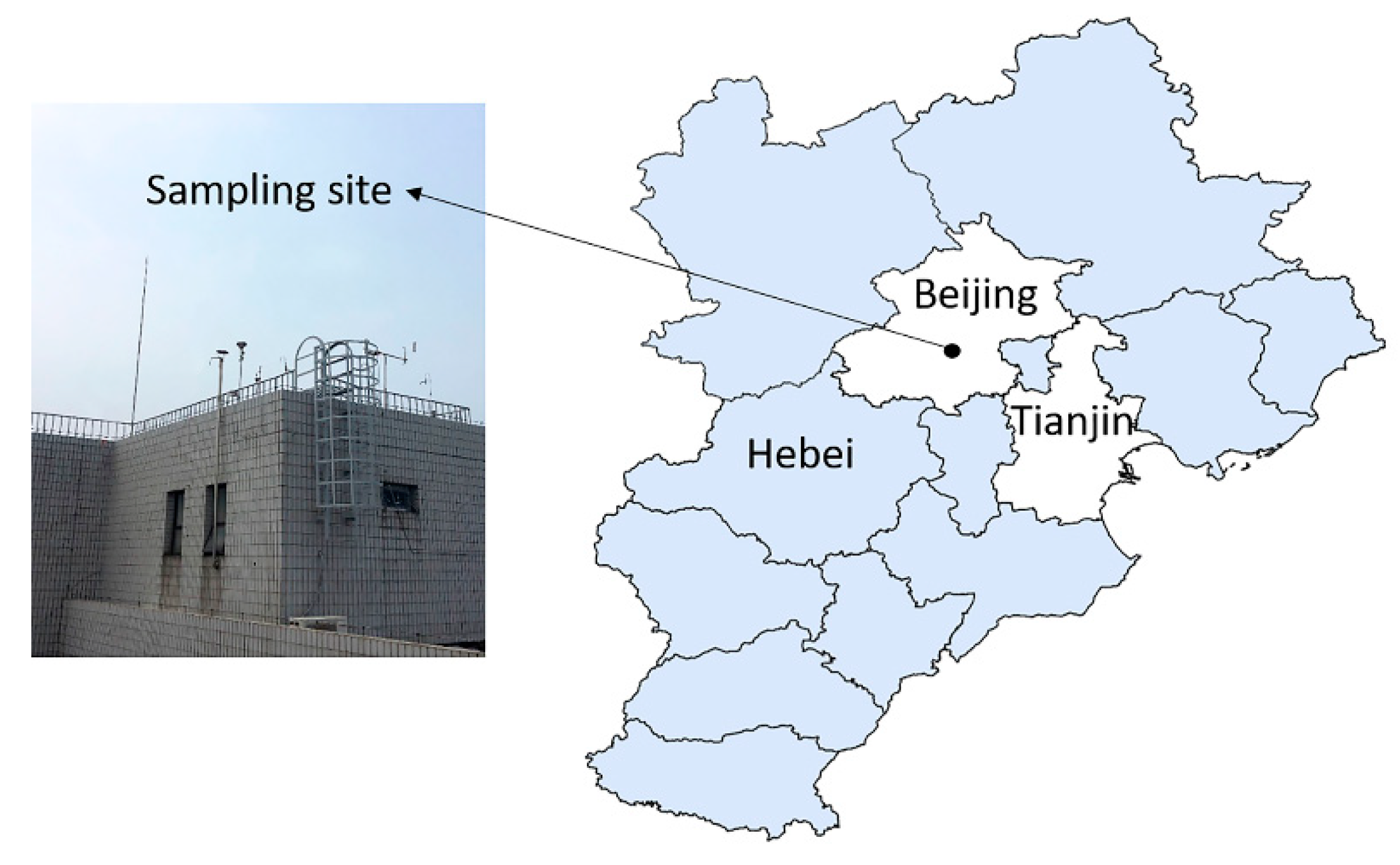
2.1. Sampling Site and High Time-Resolved Measurement

A comprehensive campaign was carried out during 16–28 March 2017 at Peking University Atmosphere Environment Monitoring Station (PKUERS) in Beijing (39°59′21″ N, 116°18′25″ E), China. The sampling site was located on the roof of an eight-story building on the campus of Peking University, about 20 m above the ground level [35] (see Figure 1). It is situated in a mixed district of commercial and residential area and can be representative of typical Beijing urban area [36]. There were no obvious emission sources in the vicinity, except two major roads (about 200 m to the east and 500 m to the south).
A set of state-of-the-art online instruments, including a PILS (ADI 2081, Metrohm AG, Herisau, Switzerland) coupled with a TOC analyzer (M9, Sievers, Boulder, Colorado, the PILS-TOC system) for near real-time WSOC monitoring (with a time resolution of two minutes), an in-situ gas and aerosol composition monitor (IGAC, Model S-630, Fortelice International Co. Ltd., Taiwan) for online measurement of water-soluble ions (e.g., Na+, K+, NH4+, Mg2+, Ca2+, NO3, Cl, NO2, SO42−), a multi-metal ambient monitor Xact (Cooper Environmental Services LLC, USA) for elements (K, Ca, V, Cr, Cu, Zn, Ga, As, Mn, Fe, Co, Ni, Se, Ag, Cd, Sn, Sb, Au, Hg, Ba, Tl, Pb, and Bi), and a semi-continuous OC and EC analyzer (Model 4, Sunset laboratory Inc., Tigard, OR, USA) were collocated. All these instruments were operated with PM2.5 inlets. Detailed descriptions for different instruments and quality assurance and quality control procedures can be found in the supplementary materials (Supporting Information Text Supplementary 1) and previous publications [26,37,38]. Briefly, WSOC concentrations in the continuous liquid samples drawn from PILS were quantified by the TOC analyzer by converting organic carbonaceous materials to carbon dioxide using chemical oxidation involving ammonium persulfate and UV light. Water-soluble ions were analyzed by an ion chromatograph (DionexICS-3000) of the IGAC system, and metals collected on the Teflon filter tape inside Xact were analyzed by nondestructive energy-dispersive X-ray fluorescence (XRF). OC and EC were analyzed using a modified National Institute for Occupational Safety and Health thermal-optical protocol (NIOSH 5040). To be noted, the time resolution of all the PM2.5 species was finally synchronized into 1 h, and the 1 h time resolution dataset was used in PMF analysis and presented in the “Results and Discussion” section.
Meteorological parameters—including temperature, relative humidity, pressure, wind speed, and wind direction—were measured by an automatic weather station during the sampling period at the observation site. Hourly PM2.5 mass concentrations were downloaded from the nearest Chinese national air quality monitoring station (Wanliu monitoring station, https://www.aqistudy.cn/).

2.2. Source Apportionment of WSOC by Positive Matrix Factorization (PMF) Model

The USEPA PMF 5.0 model was applied to quantitatively identify sources of WSOC and estimate the related source contributions during the observation period [39]. Twenty chemical species in PM2.5 were measured in this study and served as input in the PMF model for WSOC source apportionment, including WSOC, WIOC (the difference between WSOC and OC), EC, Cl, SO42−, NO3, Na+, NH4+, K, Ca, Ba, Cr, Mn, Fe, Cu, Ni, Zn, As, Se, and Pb.
Factor contributions and profiles were determined by the PMF model with a minimum value of a weighted objective function Q, which is shown in Equation (1)
Q = i = 1 n j = 1 m [ x i j k = 1 p g i k f k j u i j ] 2 ,
where xij is the concentration of species j in sample i, gik is the relative contribution of factor k to sample i (i.e., factor contribution), fkj is the concentration of species j in factor profile k (i.e., factor profile), uij is the uncertainty of species j concentration measured in sample i, p is the number of factors, n is the number of samples, and m is the number of species [40,41]. Therein, the species-specific uncertainties were calculated as a fixed fraction (5/6) of the method detection limit (MDL) if the concentration was less than or equal to the MDL. However, when the concentration was higher than the MDL, the following equation was applied:
Unc = ( E r r o r   F r a c t i o n × c o n c e n t r a t i o n ) 2 + ( 0.5 × M D L ) 2 ,
MDLs for each of the species in PMF model were listed in Table S1.
To determine the optimal number of factors, a series of tests with the number of factors ranging from four to eight were carried out, and the changes in the Q values were examined. Qexpected, Q/Qexpected and QRobust decreased when moving from four to eight factors and shared similar variations. A relatively low QRobust value was found at six factors. In addition, the uncertainty of PMF model is estimated by bootstrapping (BS), displacement (DISP), and bootstrapping with displacement (BS-DISP) [42]. At six factors, no swaps occurred with DISP and all BS-DISP runs were successfully. Therefore, six-factor solution was determined to be the optimal solution in this study.

2.3. Estimation of Secondary Organic Carbon (SOC) by the EC-Tracer Method

Secondary organic carbon (SOC) was estimated by the EC-tracer method, which was first proposed by Turpin and Huntzicker [43] and widely used in many studies [44,45]. In this method, EC is used as a tracer for primary source since EC primarily comes from incomplete combustion sources. The concentration of SOC is calculated as
OCsec = OCtot − OCpri,
OCpri = (OC/EC)pri × OC,
where OCsec is SOC, OCtot is the total OC, OCpri is primary organic carbon (POC), and (OC/EC)pri is the OC/EC ratio of aerosol from primary emissions. In this study, (OC/EC)pri was calculated by exploring the assumed independency of EC and SOC with a minimum R squared (MRS) algorithm [45,46]. With this method, SOC was calculated at each hypothetical (OC/EC)pri and the correlation coefficient (R2) of EC vs. SOC was generated. The assumed (OC/EC)pri corresponding to the minimum R2 (indicating variations of EC and SOC were independent) represented the actual (OC/EC)pri ratio. With this method, the (OC/EC)pri was determined as 2.74.
Similarly, a modified EC-tracer method was applied to estimate the amount of primary and secondary WSOC, with (WSOC/EC)pri calculated as 1.74 based on the MRS method (see Figure S1). More detailed introduction could be found in the supplementary materials (Supporting Information Text Supplmentary 2). Thus, WSOCpri was calculated by the modified EC-tracer method, which was used for comparison with WSOCpri determined by the PMF method in the following discussion section.
It should be recognized that the EC-tracer method and the modified EC-tracer method are associated with uncertainties as they are associated with certain assumptions. The results from this method were mainly used as supporting evidence and they are used for comparing with WSOC results from PMF analysis.
Besides, to identify the source regions of air masses, 72-h backward air mass trajectories were calculated by the HYSPLIT 4 trajectory model [47,48].

3. Results and Discussion

3.1. Characteristics of WSOC During the Study Period

The meteorological parameters and concentrations of carbonaceous components during the two-week observation are shown in Figure 2, and summarized in Table 1. Characteristics of carbonaceous components (e.g., OC, EC, WSOC, and WSOC/OC ratio) in this study were further compared with previous studies conducted in other cities (Table 2). The average concentration of WSOC during the study period was 5.14 ± 3.25 μg/m3, accounting for 49 ± 12% of the total OC mass, which was lower than those reported in spring of 2009 at the same sampling site (6.7 ± 1.8 μg/m3) [17], as well as in Tianjin city in Beijing–Tianjin–Hebei area (14.3 ± 11.8 μg/m3) [49], and Chengdu city (10.4 ± 3.4 μg/m3) [50]. Such differences might be attributed to the differences in sampling periods, sites and meteorological conditions, as well as the reduction of fine particulate matter level due to the implementation of clean air actions in China especially in Beijing in recent years [51]. For example, the relative humidity (RH) and temperature during this study period were significantly lower, while wind speeds were obviously higher compared to those in the study conducted in Chengdu by Tao et al. [50]. The average PM2.5 concentration level in this study was much lower compared to that in the study performed in Beijing in spring of 2009 [17], which might be related to the reduction of PM2.5 emissions with the stringent air pollutant control policies in recent years. WSOC concentrations in Beijing were much lower than those reported in Indo-Gangetic Plain of India (31.6 ± 15.3 μg/m3) [34], where biomass burning emission was a predominant source, but was still higher than those measured in European (e.g., Italy, 2 μg/m3) [26] and American cities (e.g., Atlanta, 1.98 ± 1.00 μg/m3) [52]. Carbonaceous aerosols in Atlanta were mainly influenced by biomass burning and vehicular emissions [19,20]. The WSOC/OC ratio (0.49 ± 0.12), which has been used to infer the aging of aerosols [53], was comparable to the values reported in spring in Beijing by previous studies [11,17], but much higher than the value (0.27) reported by Xiang et al. [6].
As shown in Figure 2, PM2.5 concentrations and meteorological parameters exhibited clear variations during the study period. To investigate the sources of WSOC and their changes under different pollution levels, two pollution episodes (EP1, 17–20 March, and EP2, 21–24 March) and one clean day period (CD, 25–27 March) were selected for further analysis (see Figure 2) based on PM2.5 levels. During the two EP periods, the 24-h daily average PM2.5 mass concentration was higher than 75 μg/m3, while it was less than 35 μg/m3 in CD period. Table 1 shows the average concentrations of carbonaceous components and meteorological parameters during the two EP and CD periods. It can be seen that concentrations of PM2.5 and carbonaceous components were all higher in EPs compared to CD. The average WSOC concentration during EP1 was about 9 times higher than that during CD (0.87 ± 0.21 μg/m3). In contrast to CD, EPs were characterized by lower wind speed (EPs: 2 ± 1 m/s vs. CD: 4 ± 2 m/s) and higher RH. The t-test indicated that there were statistically significant differences (at a significance level of 0.05) in most of the meteorological parameters (e.g., temperature, pressure, wind direction, and RH) and carbonaceous components and related ratios (e.g., OC, WSOC, PM2.5, EC, and OC/EC) during the two EPs. However, wind speeds and WSOC/OC ratio showed no significant differences during EP1 and EP2.

3.2. Significant Contribution of Primary Sources to WSOC

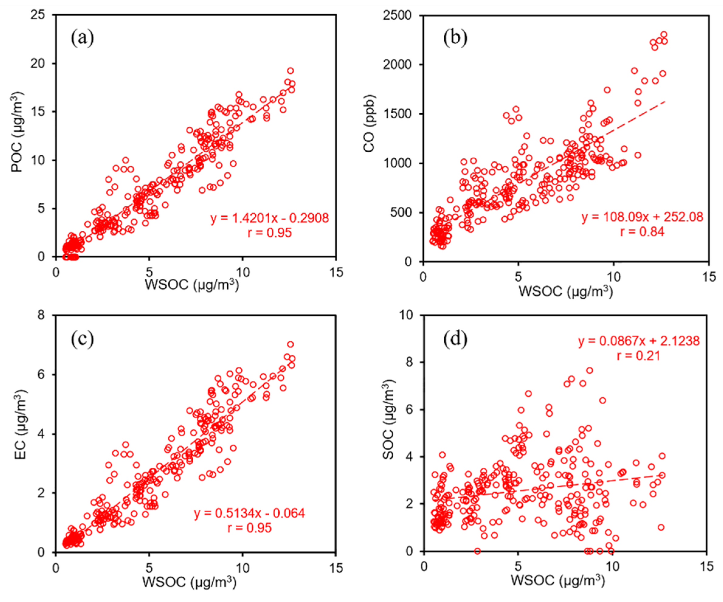
3.2.1. WSOC Highly Correlated with Primary Tracers

It can be seen from Figure 3 that during the study period, WSOC was strongly correlated with POC (p < 0.001, r = 0.95) calculated based on the EC-tracer method, and also well correlated with primary combustion source tracers such as CO (p < 0.001, r = 0.84) and EC (p < 0.001, r = 0.95) (see Figure 3a–c). By contrast, a very poor correlation (p < 0.001, r = 0.21) between WSOC and SOC was found (Figure 3d). The strong correlations of WSOC with POC, EC, and CO, as well as the extremely poor correlation between WSOC and SOC suggested that WSOC during springtime in Beijing were mainly contributed by primary sources. This was different from some previous studies conducted in Beijing, in which secondary organic aerosol was reported as the major contributor of WSOC, especially in spring and summer [11].

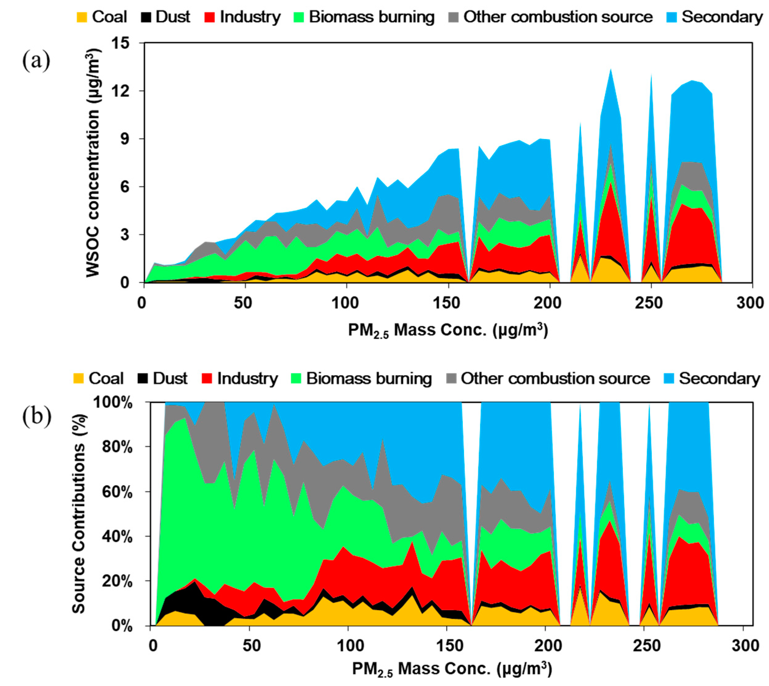
3.2.2. Primary Sources of WSOC Determined by the PMF Model

The PMF model with input number of factors varying from 4 to 8 were performed initially and finally a six-factor solution was chosen, in that six-factor solution gave the best performance. Factor profiles for the six sources, identified as coal combustion, biomass burning, industry, dust, other combustion source, and secondary sources, are shown in Figure S2. Factor 1, the coal combustion factor, had a high loading of As, Se, Pb, and moderate OC, which were typical tracers of coal combustion [55,56]. Factor 2 was characterized by two crustal elements (i.e., Ca and Ba), which could be identified as dust sources [57]. Factor 3 showed high loading of three pollution elements including Mn, Fe, and Zn, most of which may be from industrial sources [58]. Factor 4, which was characterized by K and OC, suggested biomass burning source [59]. Factor 5 was mostly loaded by EC and OC, which was identified as other combustion source including vehicle emission [60]. Factor 6 was mainly dominated by secondary inorganic ions (e.g., SO42−, NO3, and NH4+) with moderate OC, which was typical for secondary formation and included in a secondary category [61]. Na+ had relatively high loading in factor 6 probably because secondary source was mixed with some transported marine aerosol [62,63], especially in EP2. The 72-h back trajectories showed that air masses originated from marine atmosphere before reaching the receptor (Figure 4).
As shown in Figure 4, primary sources were the predominant contributors to WSOC during different periods, accounting for 68% of WSOC on average, including biomass burning (22%), other combustion source (19%), industrial source (17%), coal combustion (7%), and dust (3%). The strong correlations of WSOC with EC (p < 0.001, r = 0.95) and K (p < 0.001, r = 0.88) in Table S2 suggested that the WSOC in study period was closely related to combustion related sources especially biomass burning [36]. In addition, WSOC exhibited strong correlations with metal species such as As (correlation coefficient as 0.93), Se (0.84), Pb (0.84), Mn (0.88), Fe (0.87), and Zn (0.90), which were widely used as markers for primary and combustion related sources such as coal combustion [64,65], vehicle emission [12,36], and industrial sources [66]. Contributions of vehicle emissions and industrial sources to WSOC have been reported in Tianjin (41%) [67] and Beijing (20%) [17], respectively. However, coal combustion, a unique source of PM2.5 pollution in China compared to Europe and the U.S., showed the least contribution to WSOC (7%) in this study. This might be due to the fact that the sampling period in this study was within the non-heating period when coal combustion emission from residential sectors for central heating had been significantly reduced.
Based on PMF results, it showed clearly that primary source, instead of secondary source, was the major contributor of WSOC no matter during clean or haze days (65%). However, the relative contributions by different primary sources could vary among different periods. The relative contribution of biomass burning was obviously higher during clean period (73% on average), which was about 2 times higher than those during haze periods (EPs) (Figure 4a,b). By contrast, contributions by industry and other combustion sources were much higher during EPs, with the relative contributions increased from 0.2% and 7% in CD to 21% and 18% in EP1, respectively. The 72-h back trajectories showed that air masses reaching the monitoring site during clean days primarily originated from the northeast and northwest areas (see Figure 4c), where a large number of fires occurred (see Figure S3). Further analysis showed that the back trajectories in CD were at a relatively higher altitude, leading to the characteristics of air flow at the receptor site more similar to that of source regions. The air parcels were mainly transported from Mongolia where dust and biomass burning were important sources [68,69]. In contrast, during pollution episodes, air masses passing through the south at a lower altitude carried large amount of urban pollutants. As a result, the air masses containing more ground urban sources (e.g., industry and secondary pollutants) were observed at the receptor site (EP1 and EP2 in Figure 4). This agreed well with the results by PMF, which showed that the relative contribution of biomass burning was higher during clean period. Although, in general, the surface wind directions measured during the clean days (mostly from northwest directions) agreed well with the results of back trajectories, it should be noted there were some differences between them. The back trajectories showed north easterly and north westerly flow, while the wind direction data plot at the monitoring site during the clean days had some east/southeast/southerly flow. This is mainly because surface wind direction could be influenced by various factors such as building structure. However, air masses arriving at the monitoring site during haze days or the EPs primarily originated from the southern regions to Beijing, and passed through Hebei province and Tianjin city, which were known as heavily polluted industrial provinces [70] with urban vehicular emission contributions [67]. The distance of Tianjin City to the receptor site is about 128 km while the distance from Shijiazhuang, the capital city of Hebei Province, to the receptor site is 266 km. This explained the increased relative contributions of industrial and other combustion sources during the EPs compared to clean days, along with increased regional transport.
Furthermore, a quantitative estimate of primary WSOC and secondary WSOC based on a modified EC-tracer method (see Supporting Information Text Supplementary 2), also showed that primary WSOC dominated during the study period, accounting for about 72 ± 24% of WSOC on average (Figure 5a). Figure 5b shows primary WSOC estimated by two methods. It can be seen that the primary WSOC mass concentration calculated by the modified EC-tracer method exhibited correlation with that estimated by the PMF model during the sampling period, with r as 0.91 and a slope of 1.10. For the modified EC-tracer method, it was found that the (WSOC/EC)pri ratio varied from clean days to pollution periods, thus different ratios were applied (1.42 for EPs and 2.01 for CD) in calculating WSOCpri. Results of both methods indicated that primary sources dominated WSOC during springtime in Beijing.

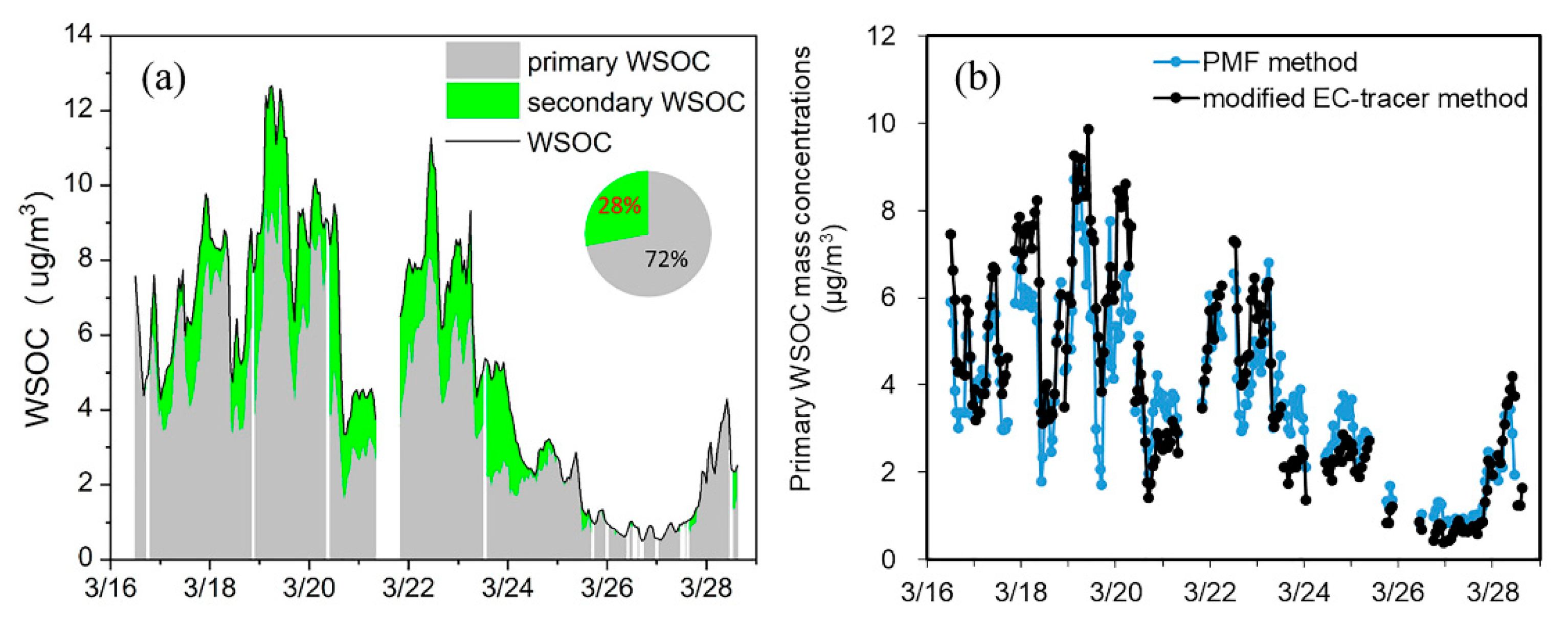
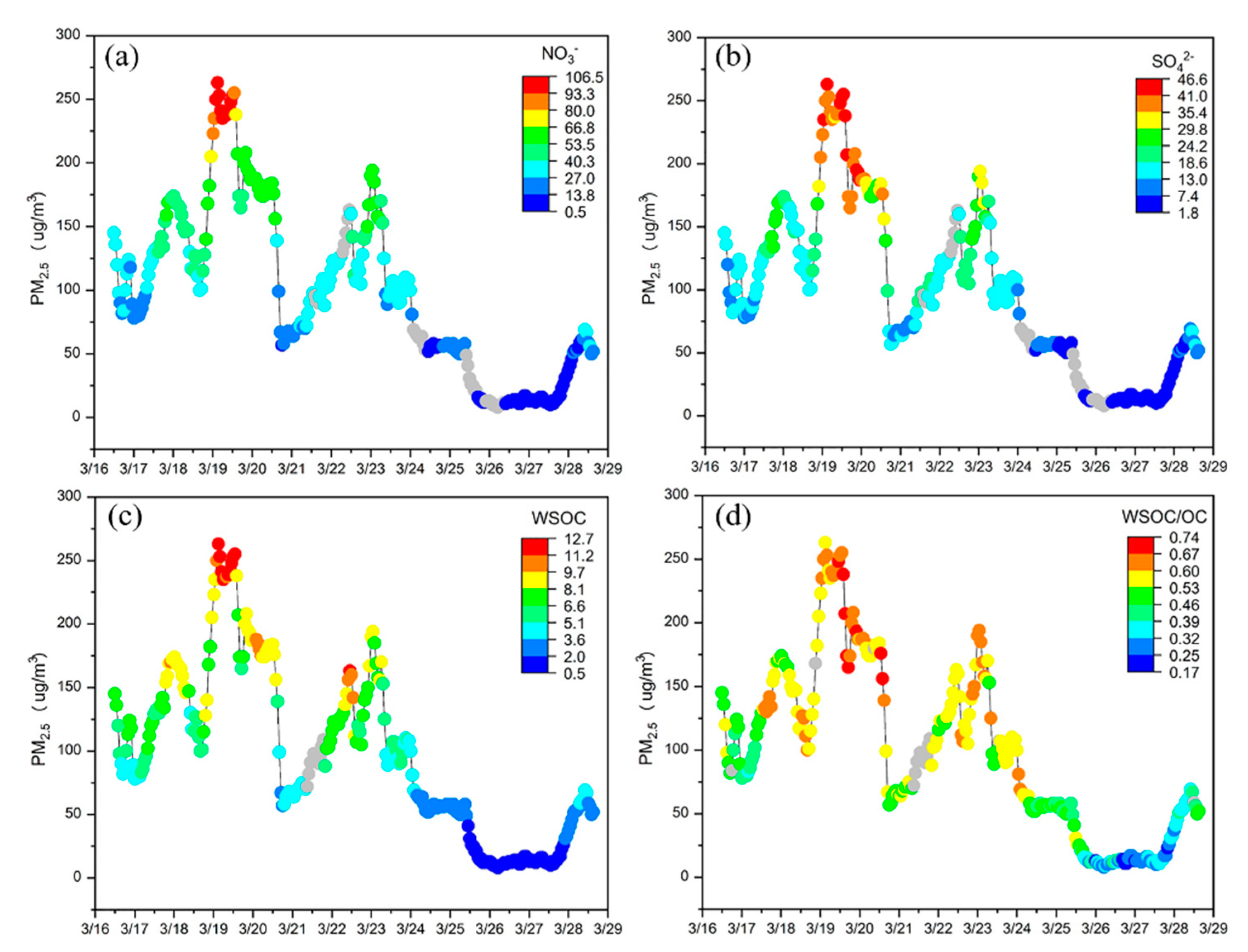
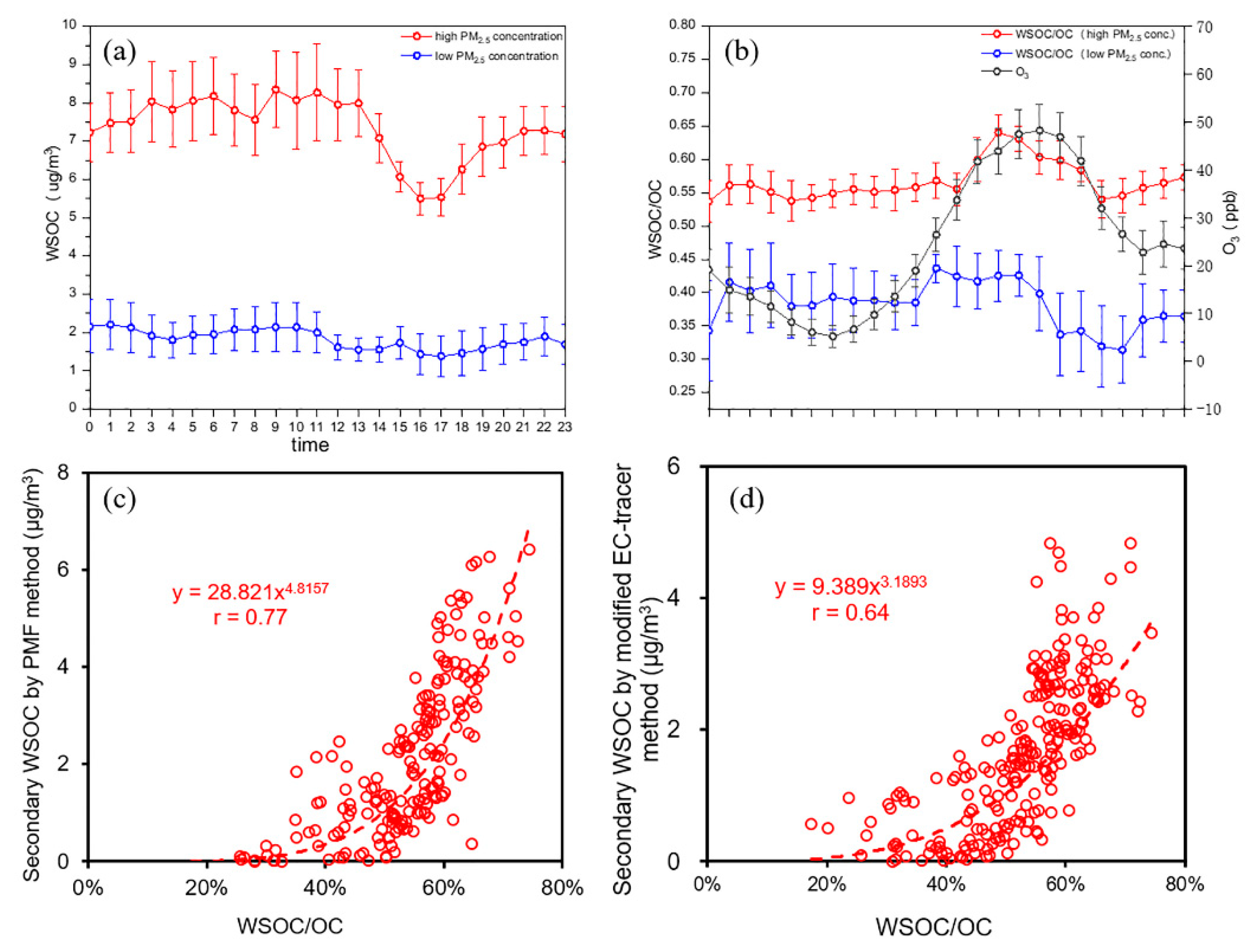
3.3. Increased Secondary Source of WSOC during Haze Episodes

As can be seen in Figure 6, the highest PM2.5 mass concentrations occurred when the highest nitrate (NO3), sulfate (SO42−), WSOC, and high WSOC/OC ratios (~0.74) were also observed. Good correlations of WSOC with SO42− (p < 0.001, r = 0.88), NO3− (p < 0.001, r = 0.93), and ammonium (p < 0.001, r = 0.89) (see Table S2) suggested that a significant fraction of the observed WSOC during the most severe haze periods could be formed via secondary formation.
The WSOC source apportionment results indicated that in general primary source played an important role in WSOC during the study period. However, Figure 7 clearly shows that secondary source contributions to WSOC gradually increased with increasing mass concentrations of PM2.5. It can be seen from Figure 4a that secondary source contributions increased from 3% during CD to around 35% during EPs. The WSOC/OC ratio varied from 0.2 to 0.4 during clean days, while it increased during EPs (in the range of 0.41–0.67), suggesting that WIOC was more enriched during clean days, while WSOC increased during haze days, primarily due to more aged aerosol and secondary source contribution.
The high time-resolved measurement also provided an opportunity to examine the hourly diurnal variations of WSOC and associated ratios, such as WSOC/OC ratio (Figure 8a,b). Generally, WSOC mass concentrations exhibited lower values in the afternoon, which were probably related to factors such as the increased mixing layer height. It is worth noting that, the WSOC/OC ratio showed a diurnal variation pattern similar to O3 with the highest WSOC/OC occurring around 14:00 p.m. in the afternoon, in both high and low PM2.5 polluted days. The high WSOC/OC ratio in the afternoon was coincident with the distribution of atmospheric O3 concentrations, indicating the presence of secondary formation [52,71].
Although WSOC is widely used as a proxy of SOA in previous studies [20,72,73], it is not the case for this study due to the high primary source contributions such as biomass burning. In addition, the WSOC/OC ratio was found to exhibit relatively good correlation with secondary WSOC quantified by PMF model (r as 0.77, see Figure 8c) and the modified EC-tracer method (r as 0.64, see Figure 8d). However, WSOC showed poor correlation with SOC (r as 0.21, see Figure 3d). This study suggested that the WSOC/OC ratio might act as a better indicator of secondary formation in cases when primary sources are the dominant source of WSOC.

4. Conclusions

High time-resolved measurements of WSOC, as well as other major components in PM2.5 were simultaneously conducted during March 2017, in Beijing. The contributions by primary and secondary WSOC were estimated for the first time based on high time-resolved monitoring data in Beijing using the modified EC-tracer method and the PMF model. Both methods agreed well that the primary source was the major source of WSOC in spring in Beijing, primarily including biomass burning, and industry sources during the study period. During pollution episodes, the relative contribution of biomass burning decreased while the contribution of secondary sources and industry increased, due to more aged aerosol and the influence of regional transport from the south of Beijing. The results from this study showed that, in some urban areas, the primary source could be the major source of WSOC; therefore, it cannot be simply used as an indicator of SOA. Future studies could cover other seasons to have a more thorough investigation of WSOC sources.

Supplementary Materials

The following are available online at https://www.mdpi.com/2073-4433/11/4/395/s1, Text S1: More detailed introduction of online measurements and related quality assurance and quality control protocols; Text S2: The modified EC-tracer method for primary and secondary WSOC estimation and related uncertainties; Figure S1: The (WSOC/EC)pri ratio determined by the MRS method; Figure S2: Source profiles of 6 factors identified by the PMF model as sources of WSOC during the study period; Figure S3. Fire maps during (a) CD, (b) EP1, and (c) EP2 provided by NASA FIRMS Web Fire Mapper; Table S1: MDL (μg/m3) for each of the species in the PMF model; Table S2: Pearson correlation coefficients of WSOC with different PM2.5 components during the study period.

Author Contributions

Conceptualization, M.Z.; Methodology, A.P.S., C.Y., and H.D; Validation, Y.J., C.Y., and M.Z.; Formal analysis, Y.J., C.Y., and Y.L.; Investigation, C.Y. and A.P.S.; Resources, A.P.S., J.L.C.J., X.W., H.D., S.C., L.Z., and M.Z.; Data curation, Y.J., C.Y., and A.P.S.; Writing—original draft preparation, Y.J. and C.Y.; Writing—review and editing, Y.J., C.Y., and M.Z.; Supervision, M.Z. All authors have read and agreed to the published version of the manuscript.

Funding

This research was funded by the National Natural Science Foundation of China (grant nos. 91744310, 41430646, 91744203). Caiqing Yan was partly supported by China Postdoctoral Science Foundation (no. 2016M590022).

Acknowledgments

The authors gratefully acknowledge the NOAA Air Resources Laboratory (ARL) for the HYSPLIT transport model.

Conflicts of Interest

The authors declare no conflict of interest.

References

  1. Kleeman, M.J.; Cass, G.R.; Eldering, A. Modeling the airborne particle complex as a source-oriented external mixture. J. Geophys. Res. Atmos. 1997, 102, 21355–21372. [Google Scholar] [CrossRef] [Green Version]
  2. Zhang, Q.; Jimenez, J.-L.; Canagaratna, M.R.; Allan, J.D.; Coe, H.; Ulbrich, I.; Alfarra, M.R.; Takami, A.; Middlebrook, A.; Sun, Y.; et al. Ubiquity and dominance of oxygenated species in organic aerosols in anthropogenically-influenced Northern Hemisphere midlatitudes. Geophys. Res. Lett. 2007, 34, L13801. [Google Scholar] [CrossRef] [Green Version]
  3. Zhang, Y.; Cai, J.; Wang, S.; He, K.; Zheng, M. Review of receptor-based source apportionment research of fine particulate matter and its challenges in China. Sci. Total Environ. 2017, 586, 917–929. [Google Scholar] [CrossRef] [PubMed]
  4. Li, C.; Chen, P.; Kang, S.; Yan, F.; Hu, Z.; Qu, B.; Sillanpää, M. Concentrations and light absorption characteristics of carbonaceous aerosol in PM 2.5 and PM 10 of Lhasa city, the Tibetan Plateau. Atmos. Environ. 2016, 127, 340–346. [Google Scholar] [CrossRef]
  5. Tang, X.; Zhang, X.; Wang, Z.; Ci, Z. Water-soluble organic carbon (WSOC) and its temperature-resolved carbon fractions in atmospheric aerosols in Beijing. Atmos. Res. 2016, 181, 200–210. [Google Scholar] [CrossRef]
  6. Xiang, P.; Zhou, X.; Duan, J.; Tan, J.; He, K.; Yuan, C.; Ma, Y.; Zhang, Y. Chemical characteristics of water-soluble organic compounds (WSOC) in PM2.5 in Beijing, China: 2011–2012. Atmos. Res. 2017, 183, 104–112. [Google Scholar] [CrossRef]
  7. Asa-Awuku, A.; Engelhart, G.J.; Lee, B.H.; Pandis, S.N.; Nenes, A. Relating CCN activity, volatility, and droplet growth kinetics of β-caryophyllene secondary organic aerosol. Atmos. Chem. Phys. 2009, 9, 795–812. [Google Scholar] [CrossRef] [Green Version]
  8. Boreddy, S.K.R.; Kawamura, K.; Mkoma, S.; Fu, P.Q. Hygroscopic behavior of water-soluble matter extracted from biomass burning aerosols collected at a rural site in Tanzania, East Africa. J. Geophys. Res. Atmos. 2014, 119, 12233–12245. [Google Scholar] [CrossRef]
  9. Hallar, A.G.; Lowenthal, D.H.; Clegg, S.L.; Samburova, V.; Taylor, N.; Mazzoleni, L.R.; Zielinska, B.; Kristensen, T.B.; Chirokova, G.; McCubbin, I.B.; et al. Chemical and hygroscopic properties of aerosol organics at Storm Peak Laboratory. J. Geophys. Res. Atmos. 2013, 118, 4767–4779. [Google Scholar] [CrossRef]
  10. Padró, L.T.; Tkacik, D.; Lathem, T.; Hennigan, C.J.; Sullivan, A.P.; Weber, R.J.; Huey, L.G.; Nenes, A.; Hennigan, C. Investigation of cloud condensation nuclei properties and droplet growth kinetics of the water-soluble aerosol fraction in Mexico City. J. Geophys. Res. Space Phys. 2010, 115, 115. [Google Scholar] [CrossRef]
  11. Du, Z.; He, K.; Cheng, Y.; Duan, F.; Ma, Y.; Liu, J.; Zhang, X.; Zheng, M.; Weber, R.J. A yearlong study of water-soluble organic carbon in Beijing I: Sources and its primary vs. secondary nature. Atmos. Environ. 2014, 92, 514–521. [Google Scholar] [CrossRef]
  12. Liu, J.; Mo, Y.; Ding, P.; Li, J.; Shen, C.; Zhang, G. Dual carbon isotopes ((14)C and (13)C) and optical properties of WSOC and HULIS-C during winter in Guangzhou, China. Sci. Total Environ. 2018, 633, 1571–1578. [Google Scholar] [CrossRef] [PubMed]
  13. Devi, J.J.; Bergin, M.H.; McKenzie, M.; Schauer, J.J.; Weber, R.J. Contribution of particulate brown carbon to light absorption in the rural and urban Southeast US. Atmos. Environ. 2016, 136, 95–104. [Google Scholar] [CrossRef] [Green Version]
  14. Hamad, S.H.; Shafer, M.M.; Kadhim, A.K.H.; Al-Omran, S.M.; Schauer, J.J. Seasonal trends in the composition and ROS activity of fine particulate matter in Baghdad, Iraq. Atmos. Environ. 2015, 100, 102–110. [Google Scholar] [CrossRef]
  15. Verma, V.; Fang, T.; Guo, H.; King, L.; Bates, J.T.; Peltier, R.E.; Edgerton, E.; Russell, A.; Weber, R.J. Reactive oxygen species associated with water-soluble PM2.5 in the southeastern United States: Spatiotemporal trends and source apportionment. Atmos. Chem. Phys. Discuss. 2014, 14, 12915–12930. [Google Scholar] [CrossRef] [Green Version]
  16. Kondo, Y.; Miyazaki, Y.; Takegawa, N.; Miyakawa, T.; Weber, R.J.; Jimenez, J.-L.; Zhang, Q.; Worsnop, D.R. Oxygenated and water-soluble organic aerosols in Tokyo. J. Geophys. Res. Space Phys. 2007, 112, 112. [Google Scholar] [CrossRef]
  17. Tao, J.; Zhang, L.; Zhang, R.; Wu, Y.; Zhang, Z.; Zhang, X.; Tang, Y.; Cao, J.; Zhang, Y. Uncertainty assessment of source attribution of PM2.5 and its water-soluble organic carbon content using different biomass burning tracers in positive matrix factorization analysis—A case study in Beijing, China. Sci. Total Environ. 2016, 543, 326–335. [Google Scholar] [CrossRef]
  18. Villalobos, A.; Amonov, M.O.; Shafer, M.M.; Devi, J.J.; Gupta, T.; Tripathi, S.N.; Rana, K.S.; McKenzie, M.; Bergin, M.H.; Schauer, J.J. Source apportionment of carbonaceous fine particulate matter (PM 2.5) in two contrasting cities across the Indo–Gangetic Plain. Atmos. Pollut. Res. 2015, 6, 398–405. [Google Scholar] [CrossRef] [Green Version]
  19. Zhang, X.; Liu, Z.; Hecobian, A.; Zheng, M.; Frank, N.H.; Edgerton, E.S.; Weber, R.J. Spatial and seasonal variations of fine particle water-soluble organic carbon (WSOC) over the southeastern United States: Implications for secondary organic aerosol formation. Atmos. Chem. Phys. Discuss. 2012, 12, 6593–6607. [Google Scholar] [CrossRef] [Green Version]
  20. Weber, R.J.; Sullivan, A.P.; Peltier, R.E.; Russell, A.; Yan, B.; Zheng, M.; De Gouw, J.; Warneke, C.; Brock, C.; Holloway, J.S.; et al. A study of secondary organic aerosol formation in the anthropogenic-influenced southeastern United States. J. Geophys. Res. Space Phys. 2007, 112, D13302. [Google Scholar] [CrossRef]
  21. Kirillova, E.N.; Andersson, A.; Han, J.; Lee, M.; Gustafsson, Ö. Sources and light absorption of water-soluble organic carbon aerosols in the outflow from northern China. Atmos. Chem. Phys. 2014, 14, 1413–1422. [Google Scholar] [CrossRef] [Green Version]
  22. Yan, C.; Zheng, M.; Bosch, C.; Andersson, A.; Desyaterik, Y.; Sullivan, A.P.; Collett, J.; Zhao, B.; Wang, S.; He, K.; et al. Important fossil source contribution to brown carbon in Beijing during winter. Sci. Rep. 2017, 7, 43182. [Google Scholar] [CrossRef]
  23. Zhang, Y.-L.; El-Haddad, I.; Huang, R.-J.; Ho, K.F.; Cao, J.; Han, Y.; Zotter, P.; Bozzetti, C.; Daellenbach, K.R.; Slowik, J.G.; et al. Large contribution of fossil fuel derived secondary organic carbon to water soluble organic aerosols in winter haze in China. Atmos. Chem. Phys. Discuss. 2018, 18, 4005–4017. [Google Scholar] [CrossRef] [Green Version]
  24. Ni, H.; Huang, R.-J.; Cao, J.; Guo, J.; Deng, H.; Dusek, U. Sources and formation of carbonaceous aerosols in Xi’an, China: Primary emissions and secondary formation constrained by radiocarbon. Atmos. Chem. Phys. 2019, 19, 15609–15628. [Google Scholar] [CrossRef] [Green Version]
  25. Sannigrahi, P.; Sullivan, A.P.; Weber, R.J.; Ingall, E.D. Characterization of water-soluble organic carbon in urban atmospheric aerosols using solid-state C-13 NMR spectroscopy. Environ. Sci. Technol. 2006, 40, 666–672. [Google Scholar] [CrossRef] [PubMed]
  26. Sullivan, A.P.; Hodas, N.; Turpin, B.J.; Skog, K.; Keutsch, F.N.; Gilardoni, S.; Paglione, M.; Rinaldi, M.; Decesari, S.; Facchini, M.C.; et al. Evidence for ambient dark aqueous SOA formation in the Po Valley, Italy. Atmos. Chem. Phys. Discuss. 2016, 16, 8095–8108. [Google Scholar] [CrossRef] [Green Version]
  27. Yan, C.; Zheng, M.; Sullivan, A.P.; Bosch, C.; Desyaterik, Y.; Andersson, A.; Li, X.; Guo, X.; Zhou, T.; Collett, J.L., Jr.; et al. Chemical characteristics and light-absorbing property of water-soluble organic carbon in Beijing: Biomass burning contributions. Atmos. Environ. 2015, 121, 4–12. [Google Scholar] [CrossRef] [Green Version]
  28. Biswas, S.; Verma, V.; Schauer, J.J.; Sioutas, C. Chemical speciation of PM emissions from heavy-duty diesel vehicles equipped with diesel particulate filter (DPF) and selective catalytic reduction (SCR) retrofits. Atmos. Environ. 2009, 43, 1917–1925. [Google Scholar] [CrossRef]
  29. Fisseha, R.; Dommen, J.; Gaeggeler, K.; Weingartner, E.; Samburova, V.; Kalberer, M.; Baltensperger, U. Online gas and aerosol measurement of water soluble carboxylic acids in Zurich. J. Geophys. Res. Space Phys. 2006, 111, 111. [Google Scholar] [CrossRef] [Green Version]
  30. Tan, J.; Zhang, L.; Zhou, X.; Duan, J.; Li, Y.; Hu, J.; He, K. Chemical characteristics and source apportionment of PM 2.5 in Lanzhou, China. Sci. Total Environ. 2017, 601, 1743–1752. [Google Scholar] [CrossRef]
  31. Van Donkelaar, A.; Martin, R.V.; Brauer, M.; Kahn, R.; Levy, R.C.; Verduzco, C.; Villeneuve, P.J. Global Estimates of Ambient Fine Particulate Matter Concentrations from Satellite-Based Aerosol Optical Depth: Development and Application. Environ. Health Perspect. 2010, 118, 847–855. [Google Scholar] [CrossRef] [PubMed] [Green Version]
  32. Tao, M.; Chen, L.; Su, L.; Tao, J. Satellite observation of regional haze pollution over the North China Plain. J. Geophys. Res. Atmos. 2012, 117, D12203. [Google Scholar] [CrossRef]
  33. Ho, K.F.; Lee, S.C.; Cao, J.; Li, Y.S.; Chow, J.C.; Watson, J.; Fung, K. Variability of organic and elemental carbon, water soluble organic carbon, and isotopes in Hong Kong. Atmos. Chem. Phys. Discuss. 2006, 6, 4569–4576. [Google Scholar] [CrossRef] [Green Version]
  34. Ram, K.; Sarin, M.M. Day-night variability of EC, OC, WSOC and inorganic ions in urban environment of Indo-Gangetic Plain: Implications to secondary aerosol formation. Atmos. Environ. 2011, 45, 460–468. [Google Scholar] [CrossRef]
  35. Liu, Y.; Yan, C.; Zheng, M. Source apportionment of black carbon during winter in Beijing. Sci. Total Environ. 2018, 618, 531–541. [Google Scholar] [CrossRef] [PubMed]
  36. Liu, Y.; Zheng, M.; Yu, M.; Cai, X.; Du, H.; Li, J.; Zhou, T.; Yan, C.; Wang, X.; Shi, Z.; et al. High-time-resolution source apportionment of PM2.5 in Beijing with multiple models. Atmos. Chem. Phys. Discuss. 2019, 19, 6595–6609. [Google Scholar] [CrossRef] [Green Version]
  37. Sullivan, A.P.; Peltier, R.E.; Brock, C.; De Gouw, J.; Holloway, J.S.; Warneke, C.; Wollny, A.G.; Weber, R.J. Airborne measurements of carbonaceous aerosol soluble in water over northeastern United States: Method development and an investigation into water-soluble organic carbon sources. J. Geophys. Res. Space Phys. 2006, 111, D23S46. [Google Scholar] [CrossRef]
  38. Zhang, B.; Zhou, T.; Liu, Y.; Yan, C.; Li, X.; Yu, J.; Wang, S.; Liu, B.; Zheng, M. Comparison of water-soluble inorganic ions and trace metals in PM2.5 between online and offline measurements in Beijing during winter. Atmos. Pollut. Res. 2019, 10, 1755–1765. [Google Scholar] [CrossRef]
  39. Paterson, K.G.; Sagady, J.L.; Hooper, D.L. Analysis of Air Quality Data Using Positive Matrix Factorization. Environ. Sci. Technol. 1999, 33, 635–641. [Google Scholar] [CrossRef]
  40. Paatero, P. Least squares formulation of robust non-negative factor analysis. Chemometr. Intell. Lab. 1997, 37, 23–35. [Google Scholar] [CrossRef]
  41. Norris, G.; Duvall, R.; Brown, S.; Bai, S. EPA Positive Matrix Factorization (PMF) 5.0 Fundamentals and User Guide; U.S. Environmental Protection Agency: Washington, DC, USA, 2014.
  42. Brown, S.G.; Eberly, S.; Paatero, P.; Norris, G.A. Methods for estimating uncertainty in PMF solutions: Examples with ambient air and water quality data and guidance on reporting PMF results. Sci. Total Environ. 2015, 518–519, 626–635. [Google Scholar] [CrossRef] [PubMed] [Green Version]
  43. Turpin, B.J.; Huntzicker, J.J. Identification of secondary organic aerosol episodes and quantitation of primary and secondary organic aerosol concentrations during SCAQS. Atmos. Environ. 1995, 29, 3527–3544. [Google Scholar] [CrossRef]
  44. Srivastava, D.; Favez, O.; Perraudin, E.; Villenave, E.; Albinet, A. Comparison of Measurement-Based Methodologies to Apportion Secondary Organic Carbon (SOC) in PM2.5: A Review of Recent Studies. Atmosphere 2018, 9, 452. [Google Scholar] [CrossRef] [Green Version]
  45. Wu, C.; Yu, J.Z. Determination of primary combustion source organic carbon-to-elemental carbon (OC / EC) ratio using ambient OC and EC measurements: Secondary OC-EC correlation minimization method. Atmos. Chem. Phys. 2016, 16, 5453–5465. [Google Scholar] [CrossRef] [Green Version]
  46. Wu, C.; Wu, D.; Yu, J.Z. Quantifying black carbon light absorption enhancement with a novel statistical approach. Atmos. Chem. Phys. 2018, 18, 289–309. [Google Scholar] [CrossRef] [Green Version]
  47. Rolph, G.; Stein, A.; Stunder, B. Real-time Environmental Applications and Display sYstem: READY. Environ. Modell. Softw. 2017, 95, 210–228. [Google Scholar] [CrossRef]
  48. Stein, A.F.; Draxler, R.R.; Rolph, G.D.; Stunder, B.J.B.; Cohen, M.D.; Ngan, F. NOAA’s HYSPLIT atmospheric transport and dispersion modeling system. Bull. Am. Meteorol. Soc. 2015, 96, 2059–2077. [Google Scholar] [CrossRef]
  49. Xu, W.; Fu, Z.M.; Chen, J.X.; Tian, H. Ground-Based Measurement and Variation Analysis of Carbonaceous Aerosols in Wuqing. Acta Sci. Natur. Univ. Pekin. 2016, 52. [Google Scholar] [CrossRef]
  50. Tao, J.; Zhang, L.; Engling, G.; Zhang, R.; Yang, Y.; Cao, J.; Zhu, C.; Wang, Q.; Luo, L. Chemical composition of PM2.5 in an urban environment in Chengdu, China: Importance of springtime dust storms and biomass burning. Atmos. Res. 2013, 122, 270–283. [Google Scholar] [CrossRef]
  51. Zheng, B.; Tong, D.; Li, M.; Liu, F.; Hong, C.; Geng, G.; Li, H.; Li, X.; Peng, L.; Qi, J.; et al. Trends in China’s anthropogenic emissions since 2010 as the consequence of clean air actions. Atmos. Chem. Phys. Discuss. 2018, 18, 14095–14111. [Google Scholar] [CrossRef] [Green Version]
  52. Sullivan, A.P.; Weber, R.J.; Clements, A.L.; Turner, J.R.; Bae, M.S.; Schauer, J.J. A method for on-line measurement of water-soluble organic carbon in ambient aerosol particles: Results from an urban site. Geophys. Res. Lett. 2004, 31, L13105. [Google Scholar] [CrossRef] [Green Version]
  53. Cho, S.Y.; Park, S.S. Resolving sources of water-soluble organic carbon in fine particulate matter measured at an urban site during winter. Environ. Sci. Proc. Impact 2013, 15, 524–534. [Google Scholar] [CrossRef]
  54. Pathak, R.K.; Wang, T.; Ho, K.F.; Lee, S.C. Characteristics of summertime PM2.5 organic and elemental carbon in four major Chinese cities: Implications of high acidity for water-soluble organic carbon (WSOC). Atmos. Environ. 2011, 45, 318–325. [Google Scholar] [CrossRef]
  55. Vejahati, F.; Xu, Z.; Gupta, R. Trace elements in coal: Associations with coal and minerals and their behavior during coal utilization—A review. Fuel 2010, 89, 904–911. [Google Scholar] [CrossRef]
  56. Xu, H.; Cao, J.; Ho, K.F.; Ding, H.; Han, Y.; Wang, G.; Chow, J.; Watson, J.; Khol, S.; Qiang, J.; et al. Lead concentrations in fine particulate matter after the phasing out of leaded gasoline in Xi’an, China. Atmos. Environ. 2012, 46, 217–224. [Google Scholar] [CrossRef]
  57. Amato, F.; Schaap, M.; Van Der Gon, H.D.; Pandolfi, M.; Alastuey, A.; Keuken, M.; Querol, X. Short-term variability of mineral dust, metals and carbon emission from road dust resuspension. Atmos. Environ. 2013, 74, 134–140. [Google Scholar] [CrossRef]
  58. Yu, L. Characterization and Source Apportionment of PM2.5 in an Urban Environment in Beijing. Aerosol Air Qual. Res. 2013, 13, 574–583. [Google Scholar] [CrossRef] [Green Version]
  59. Duan, F.; Liu, X.; Yu, T.; Cachier, H. Identification and estimate of biomass burning contribution to the urban aerosol organic carbon concentrations in Beijing. Atmos. Environ. 2004, 38, 1275–1282. [Google Scholar] [CrossRef]
  60. Kim, E.; Hopke, P.K.; Edgerton, E.S. Source Identification of Atlanta Aerosol by Positive Matrix Factorization. J. Air Waste Manag. Assoc. 2003, 53, 731–739. [Google Scholar] [CrossRef] [Green Version]
  61. Gao, J.; Peng, X.; Chen, G.; Xu, J.; Shi, G.-L.; Zhang, Y.-C.; Feng, Y.-C. Insights into the chemical characterization and sources of PM2.5 in Beijing at a 1-h time resolution. Sci. Total. Environ. 2016, 542, 162–171. [Google Scholar] [CrossRef]
  62. Ashrafi, K.; Fallah, R.; Hadei, M.; Yarahmadi, M.; Shahsavani, A. Source Apportionment of Total Suspended Particles (TSP) by Positive Matrix Factorization (PMF) and Chemical Mass Balance (CMB) Modeling in Ahvaz, Iran. Arch. Environ. Contam. Toxicol. 2018, 75, 278–294. [Google Scholar] [CrossRef] [PubMed]
  63. Santoso, M.; Hopke, P.K.; Hidayat, A.; Diah Dwiana, L. Sources identification of the atmospheric aerosol at urban and suburban sites in Indonesia by positive matrix factorization. Sci. Total Environ. 2008, 397, 229–237. [Google Scholar] [CrossRef] [PubMed]
  64. Deng, S.; Shi, Y.; Liu, Y.; Zhang, C.; Wang, X.; Cao, Q.; Li, S.; Zhang, F. Emission characteristics of Cd, Pb and Mn from coal combustion: Field study at coal-fired power plants in China. Fuel Process. Technol. 2014, 126, 469–475. [Google Scholar] [CrossRef]
  65. Tian, H.; Wang, Y.; Xue, Z.G.; Cheng, K.; Qu, Y.P.; Chai, F.H.; Hao, J.M. Trend and characteristics of atmospheric emissions of Hg, As, and Se from coal combustion in China, 1980–2007. Atmos. Chem. Phys. Discuss. 2010, 10, 11905–11919. [Google Scholar] [CrossRef] [Green Version]
  66. Zheng, M.; Zhang, Y.; Yan, C.; Fu, H.; Niu, H.; Huang, K.; Fu, Q. Establishing PM2.5 industrial source profiles in Shanghai. China Environ. Sci. 2013, 33, 1354–1359. [Google Scholar]
  67. Wen, J.; Shi, G.; Tian, Y.; Chen, G.; Liu, J.; Huang-Fu, Y.; Ivey, C.E.; Feng, Y. Source contributions to water-soluble organic carbon and water-insoluble organic carbon in PM2.5 during Spring Festival, heating and non-heating seasons. Ecotoxicol. Environ. Saf. 2018, 164, 172–180. [Google Scholar] [CrossRef]
  68. Jugder, D.; Sugimoto, N.; Shinoda, M.; Kimura, R.; Matsui, I.; Nishikawa, M. Dust, biomass burning smoke, and anthropogenic aerosol detected by polarization-sensitive Mie lidar measurements in Mongolia. Atmos. Environ. 2012, 54, 231–241. [Google Scholar] [CrossRef]
  69. Lee, K.Y.; Batmunkh, T.; Joo, H.S.; Park, K. Comparison of the physical and chemical characteristics of fine road dust at different urban sites. J. Air Waste Manag. Assoc. 2018, 68, 812–823. [Google Scholar] [CrossRef] [Green Version]
  70. Wang, L.; Zhang, F.; Pilot, E.; Yu, J.; Nie, C.; Holdaway, J.; Yang, L.; Li, Y.; Wang, W.; Vardoulakis, S.; et al. Taking Action on Air Pollution Control in the Beijing-Tianjin-Hebei (BTH) Region: Progress, Challenges and Opportunities. Int. J. Environ. Res. Public Health 2018, 15, 306. [Google Scholar] [CrossRef] [Green Version]
  71. Kaul, D.S.; Gupta, T.; Tripathi, S.N.; Tare, V.; Collett, J.L. Secondary Organic Aerosol: A Comparison between Foggy and Nonfoggy Days. Environ. Sci. Technol. 2011, 45, 7307–7313. [Google Scholar] [CrossRef]
  72. Hennigan, C.J.; Bergin, M.H.; Russell, A.G.; Nenes, A.; Weber, R.J. Gas/particle partitioning of water-soluble organic aerosol in Atlanta. Atmos. Chem. Phys. 2009, 9, 3613–3628. [Google Scholar] [CrossRef] [Green Version]
  73. Rastogi, N.; Patel, A.; Singh, A.; Singh, D. Diurnal Variability in Secondary Organic Aerosol Formation over the Indo-Gangetic Plain during Winter Using Online Measurement of Water-Soluble Organic Carbon. Aerosol Air Qual. Res. 2015, 15, 2225–2231. [Google Scholar] [CrossRef] [Green Version]
Figure 1. Location of the sampling site in this study.
Atmosphere 11 00395 g001
Figure 2. Time series of concentrations of (a) PM2.5, (b) OC, EC, and WSOC, (c) ratios of WSOC/OC and WIOC/OC, and (df) meteorological parameters during the study period, including two pollution episodes (EP1 and EP2) and one clean day (CD) period. Note: The dashed black and light blue lines indicate PM2.5 levels of 75 μg/m3 and 35 μg/m3, respectively. The gray and light blue shaded areas refer to the EP and CD periods, respectively. OC: Organic carbon, WSOC: water-soluble organic carbon, EC: elemental carbon.
Atmosphere 11 00395 g002
Figure 3. Correlations of WSOC with (a) POC, (b) CO, (c) EC, and (d) SOC.
Atmosphere 11 00395 g003
Figure 4. Source contribution to the observed WSOC during clean days (CD) and pollution episodes (EP) based on PMF model: (a) average source contribution, (b) temporal variation of different source contributions and the WSOC/OC ratio (blue line, in percentage), and (c) 72-h backward air mass trajectories.
Atmosphere 11 00395 g004
Figure 5. (a) Time series of WSOC from primary and secondary sources and their average contributions during the study period, which was calculated by the modified EC-tracer method. (b) Primary WSOC estimated by the modified EC-tracer method and the PMF method.
Atmosphere 11 00395 g005
Figure 6. Temporal variation of PM2.5 colored by (a) NO3, (b) SO42, (c) WSOC, and (d) the WSOC/OC ratio during the study period. Note: gray dots represent missing data.
Atmosphere 11 00395 g006
Figure 7. Variation of (a) absolute and (b) relative contributions of different sources to WSOC with PM2.5 concentrations.
Atmosphere 11 00395 g007
Figure 8. Diurnal variations of (a) WSOC and (b) WSOC/OC ratio under high and low PM2.5 concentrations and average concentration of O3; and correlations between the WSOC/OC ratio with secondary WSOC calculated by (c) PMF results and (d) modified EC-tracer method. Note: High PM2.5 concentration condition is defined by days with daily PM2.5 concentration higher than 75 μg/m3, while those lower than 75 μg/m3 are defined as low PM2.5 concentration condition.
Atmosphere 11 00395 g008
Table 1. Summary of mass concentrations of different carbonaceous components and meteorological conditions during the study period. OC: Organic carbon, WSOC: water-soluble organic carbon, EC: elemental carbon. EP1 and EP2: two pollution episodes, CD: clean day.
AverageEP1EP2CD
Average ± Standard Deviation (Median)Sample Number (N)Average ± Standard Deviation (Median)Sample Number (N)Average ± Standard Deviation (Median)Sample Number (N)Average ± Standard Deviation (Median)Sample Number (N)
Temperature (°C)10 ± 4
(10)
29212 ± 3
(12)
908 ± 3
(7)
8810 ± 3
(10)
51
Pressure (hPa)1013 ± 2
(1012)
2921013 ± 3
(1013)
901014 ± 3
(1015)
881012 ± 1
(1012)
51
Wind speed (m/s)2 ± 1
(2)
2922 ± 1
(2)
902 ± 1
(2)
884 ± 2
(4)
51
Wind direction (°)201 ± 70
(199)
292162 ± 61
(165)
90200 ± 71
(207)
88263 ± 55
(286)
51
Relative humidity (%)51 ± 22
(46)
29248 ± 13
(47)
9067 ± 18
(75)
8831 ± 10
(32)
51
PM2.5 (μg/m3)98 ± 68
(91)
283164 ± 56
(163)
90109 ± 37
(102)
8813 ± 3
(13)
51
WSOC (μg/m3)5.14 ± 3.25 (4.89)2818.14 ± 2.17
(8.39)
906.05 ± 2.16 (5.33)770.87 ± 0.21 (0.86)51
OC (μg/m3)9.54 ± 4.98 (9.01)28714.01 ± 3.43 (14.59)8810.47 ± 3.39 (9.32)872.80 ± 0.50 (2.67)51
EC (μg/m3)2.63 ± 1.71 (2.35)2764.14 ± 1.40
(4.24)
882.70 ± 1.27
(2.18)
870.46 ± 0.13 (0.45)40
WSOC/OC0.49 ± 0.12 (0.52)2760.58 ± 0.08
(0.59)
880.56 ± 0.05
(0.56)
760.31 ± 0.06 (0.31)51
OC/EC4.38 ± 1.31 (4.12)2763.56 ± 0.72
(3.35)
884.20 ± 0.88
(4.07)
876.20 ± 1.31 (6.12)40
Table 2. Concentrations (μg/m3) and ratios of carbonaceous components reported in different studies.
CitySeasonsSampling MethodECOCWSOCWSOC/OCReferences
BeijingSpring 2017Online PILS-TOC2.63 ± 1.719.54 ± 4.985.14 ± 3.250.49 ± 0.12This study
BeijingSpring 2009
Summer 2009
Autumn 2009
Winter 2009
Offline TOC2.8 ± 1.113.7 ± 4.46.7 ± 1.8 [17]
4.2 ± 1.211.1 ± 1.83.2 ± 1.1
5.3 ± 2.817.8 ± 5.67.7 ± 5.0
7.5 ± 7.424.9 ± 15.67.7 ± 3.6
BeijingSummer 2011
Autumn 2011
Winter 2011
Spring 2012
Summer 2012
Offline TOC3.0813.554.480.33[6]
5.425.425.820.25
4.728.165.530.2
2.9816.573.90.27
3.1516.545.810.34
BeijingSummer 2013
Winter 2012
Offline TOC1.90 ± 0.639.65 ± 2.876.42 ± 2.170.66 ± 0.06[27]
5.58 ± 1.4432.9 ± 16.810.8 ± 3.130.39 ± 0.16
TianjinWinter 2011Online PILS-TOC6.0 ± 4.821.5 ± 19.214.3 ± 11.8 [49]
Beijing
Shanghai
Lanzhou
Guangzhou
Summer 2005
Spring 2005
Summer 2006
Spring 2004
Offline TOC4.9 ± 2.98.2 ± 3.74.5 ± 2.30.55 ± 0.1[54]
10.0 ± 5.516.9 ± 12.25.8 ± 4.20.35 ± 0.1
2.9 ± 1.46.6 ± 2.92.4 ± 0.80.4 ± 0.1
10.5 ± 3.714.9 ± 5.84.3 ± 1.20.32 ± 0.1
ChengduSpring 2009Offline TOC5.7 ± 1.820.7 ± 6.010.4 ± 3.40.5[50]
AtlantaSummer 2004Online PILS-TOC 3.22 ± 1.121.98 ± 1.000.60 ± 0.13[37]
KanpurAutumn 2008Offline TOC7.7 ± 2.947 ± 2131.6 ± 15.30.66 ± 0.10 (day) 0.47 ± 0.07 (night)[34]

