Review

What Polarimetric Weather Radars Offer to Cloud Modelers: Forward Radar Operators and Microphysical/Thermodynamic Retrievals

1
Cooperative Institute for Mesoscale Meteorological Studies, University of Oklahoma, Norman, OK 73072, USA
2
NOAA/OAR National Severe Storms Laboratory, Norman, OK 73072, USA
3
Institute of Earth Sciences, The Hebrew University of Jerusalem, Jerusalem 9190401, Israel
*
Author to whom correspondence should be addressed.
Atmosphere 2020, 11(4), 362; https://doi.org/10.3390/atmos11040362
Submission received: 22 January 2020 / Revised: 1 April 2020 / Accepted: 5 April 2020 / Published: 8 April 2020
(This article belongs to the Special Issue Electromagetics and Polarimetric Weather Radar)

Abstract

:
The utilization of polarimetric weather radars for optimizing cloud models is a next frontier of research. It is widely understood that inadequacies in microphysical parameterization schemes in numerical weather prediction (NWP) models is a primary cause of forecast uncertainties. Due to its ability to distinguish between hydrometeors with different microphysical habits and to identify “polarimetric fingerprints” of various microphysical processes, polarimetric radar emerges as a primary source of needed information. There are two approaches to leverage this information for NWP models: (1) radar microphysical and thermodynamic retrievals and (2) forward radar operators for converting the model outputs into the fields of polarimetric radar variables. In this paper, we will provide an overview of both. Polarimetric measurements can be combined with cloud models of varying complexity, including ones with bulk and spectral bin microphysics, as well as simplified Lagrangian models focused on a particular microphysical process. Combining polarimetric measurements with cloud modeling can reveal the impact of important microphysical agents such as aerosols or supercooled cloud water invisible to the radar on cloud and precipitation formation. Some pertinent results obtained from models with spectral bin microphysics, including the Hebrew University cloud model (HUCM) and 1D models of melting hail and snow coupled with the NSSL forward radar operator, are illustrated in the paper.

1. Introduction

Doppler polarimetric radars have become the standard for operational weather radars around the world. Compared to single-polarization radars, dual-polarization radars substantially improve data quality, precipitation estimation, hydrometeor classification, and severe weather warnings. Comprehensive overviews of radar polarimetry and its utilization for weather observations are described in the monographs of Bringi and Chandrasekar [1], Zhang [2] and Ryzhkov and Zrnic [3].
The utilization of polarimetric weather radars to optimize numerical weather prediction (NWP) models is a new frontier of research. It is widely understood that inadequate microphysical parameterization schemes in NWP models are a primary source of forecast uncertainties (e.g., Morrison et al. [4] and Fan et al. [5]). Observational data provided by ground-based weather surveillance and cloud radars, lidars, radiometers, and airborne or spaceborne remote sensors are crucial for constraining model microphysical schemes. Due to its ability to distinguish between hydrometeors with different microphysical habits and to identify the “polarimetric fingerprints” of various microphysical processes, polarimetric radar has emerged as an important source of needed information.
The purpose of this paper is to provide a review of some of the important information that polarimetric weather radars can provide that may be of use to the cloud modeling community. We hope that through increased awareness of polarimetric radar forward operators, microphysical and thermodynamic retrievals and other polarimetric products and data can be integrated into cloud models through improved data assimilation and leveraged to assess and validate numerical models and/or microphysics schemes.
In this review, we will focus on the applications of longer-wavelength polarimetric radars operating at centimeter radar wavelengths at S, C, and X microwave frequency bands which commonly comprise operational weather radar networks around the world. These radars are used for surveillance of large areas with extended radar coverage as opposed to cloud radars operating at millimeter wavelengths at Ka- or W-band frequencies. Weather surveillance radars do not have sufficient sensitivity to detect echoes from atmospheric aerosols or cloud particles (liquid or solid) with sizes less than 50–100 microns but have great advantage for remote sensing of deep convective storms containing large hydrometeors producing prohibitively strong attenuation at cloud radar frequencies. Although centimeter-wavelength radars do not see small cloud droplets, they are often capable of detecting non-precipitating clouds containing ice or clear-air turbulence associated with Bragg scattering. Melnikov et al. [6] claim that longer-wavelength operational radars such as WSR-88D in the US have the potential to be used as “cloud radars”.
In addition to the three radar variables commonly measured by single-polarization Doppler radars (i.e., radar reflectivity Z, mean Doppler velocity, and Doppler spectrum width), polarimetric radars can provide estimates of differential reflectivity ZDR, specific differential phase KDP, linear depolarization ratio (LDR), cross-correlation coefficient ρhv, specific attenuation A, and specific differential attenuation ADP. For definitions and the physical meanings of these polarimetric variables, a reader can consult basic monographs [1,2,3]. Using such multi-parameter measurements, one can discriminate between hydrometeors with different shapes, orientations, and phase compositions; reduce uncertainties in the retrievals of size distributions of atmospheric particles that are generally characterized by at least three parameters; and identify polarimetric signatures attributed to different microphysical processes. These include the evaporation, coalescence, and breakup of raindrops; depositional growth, sublimation, and aggregation of ice/snow; and the processes involving mixed-phase hydrometeors such as melting, freezing, refreezing, and riming. Although the processes of cloud and ice nucleation and the initial condensation growth of small particles are invisible to the radar, their impacts can be indirectly identified through their influence on the polarimetric characteristics of clouds at later stages of cloud development when larger particles are formed. It is noteworthy that multiple polarimetric variables are measured in the same radar resolution volume as opposed to multi-frequency measurements from multiple radars, for which the matching of the sampling volumes is always a challenge. This is a reason why multi-frequency retrievals of microphysical and thermodynamic characteristics of clouds with ground-based radars are primarily confined in the research domain whereas polarimetric radar retrievals can be easily implemented on existing operational radar networks. Of course, the use of polarimetric radars in conjunction with cloud models is still a subject of exploratory research, but we believe that operational polarimetric radars are a primary resource for optimizing NWP models on a national scale in the foreseeable future.
There are two approaches for incorporating information from dual-polarization radars into NWP models: (1) microphysical and thermodynamic retrievals from radar (which is a way of converting radar information into quantities that the model prognoses) and (2) forward operators that convert the model output into polarimetric radar fields. In this paper, we will provide an overview of both. The idea of using forward operators for assimilating polarimetric radar information into NWP models is also explored in the recent article of Zhang et al. [7]. The Zhang et al. paper focuses on a unified statistical approach for model performance optimization based on synthesizing observation-based retrievals and model analyses. Such an approach requires knowledge of the background error covariance and observation error covariance stipulated by the theory of optimal estimation. In our article, we focus exclusively on the direct, observation-based retrievals (microphysical and thermodynamic) using polarimetric radar data.
The paper is organized as follows. We begin with a general overview of the electromagnetic model of scattering and forward operators in Section 2. The microphysical and thermodynamic radar retrievals are described in Section 3 and Section 4, respectively, followed by conclusions in Section 5. Formulas for computing different polarimetric radar variables from the output of cloud models are in the Appendix A.

2. Electromagnetic Model of Scattering and Forward Operators

2.1. Scattering by Individual Hydrometeor

The polarimetric properties of most meteorological scatterers are generally well-quantified if they are modeled as spheroids with oblate or prolate shapes. The characteristics of electromagnetic scattering by spheroidal particles depend on their size, shape, orientation, and physical composition and are described in terms of the scattering matrix S, which has the following form for a single spheroidal hydrometeor with an axis of symmetry a and transverse axis b (Holt [8], Ryzhkov [9], and Ryzhkov and Zrnic [3]):
S = [ ( s a ( π ) s b ( π ) ) sin 2 ψ sin 2 α + s b ( π ) ( s a ( π ) s b ( π ) ) sin 2 ψ sin α cos α ( s a ( π ) s b ( π ) ) sin 2 ψ sin α cos α ( s a ( π ) s b ( π ) ) sin 2 ψ cos 2 α + s b ( π ) ]
In Equation (1), sa(π) is the backscattering amplitude if the electric field vector of the incident electromagnetic wave is parallel to the symmetry axis of the hydrometeor, and sb(π) stands for the backscattering amplitude if the electric field vector is perpendicular to the symmetry axis. Angles α and Ψ characterize the orientation of the spheroid and are illustrated in Figure 1. Strictly speaking, expression (1) for S is valid for particles such as raindrops at radar frequencies up to 35 GHz provided that Ψ > 80° (Holt and Shepherd [10]), but it can be universally applied at lower frequencies for the majority of practical applications. For more rigorous modeling of scattering by spheroids, the reader is referred to Vivekanandan et al. [11].
If the electromagnetic waves transmitted and received by the radar propagate in a medium filled with nonspherical hydrometeors, the complex voltages of the radar return at orthogonal polarizations depend not only on the elements of the scattering matrix S of the hydrometeor but also on the polarization properties of the propagation medium characterized by the transmission matrix T. The resulting voltage vector Vr of the received signal is given by (Ryzhkov and Zrnic [3]).
V r = T S T V t
where Vt is the voltage vector characterizing a transmitted wave. Whereas the scattering matrix S is characterized by the “backscattering” amplitudes sa(π) and sb(π) for the scatterer in the radar resolution volume, the transmission matrix T is determined by the “forward scattering” amplitudes sa(0) and sb(0) of the scatterers located along the propagation path (e.g., Bringi and Chandrasekar [1], Zhang [2], and Ryzhkov and Zrnic [3]).
If the hydrometeors are relatively small compared to the radar wavelength λ and are modeled as oblate or prolate spheroids, then simple analytical formulas for the forward scattering and backscattering amplitudes s a ( 0 , π ) and s b ( 0 , π ) can be obtained in the Rayleigh approximation (Van de Hulst [12]):
s a , b ( 0 ) = s a , b ( π ) = π 2 D 3 6 λ 2 1 L a , b + 1 ε 1 ,
where D = (ab2)1/3 is the equivolume diameter of the particle, ε is its dielectric constant, and La and Lb are the shape parameters defined as
L a = 1 + f 2 f 2 ( 1 arctan f f ) , f = b 2 a 2 1 , L b = 1 L a 2 ,
for oblate spheroids (a < b) and
L a = 1 e 2 e 2 ( 1 2 e ln ( 1 e 1 e ) 1 ) , e = 1 b 2 a 2 , L b = 1 L a 2 ,
for prolate spheroids (a > b).
The dielectric constant ε is a function of the radar wavelength; phase composition (e.g., water, ice, air, or some combination thereof); temperature; and density of the scattering material. For mixed-phase particles, ε depends on the relative fractions of water, solid ice, and air, with various mixing formulas used for computing ε of such hydrometeors, the most popular of which were suggested by Maxwell Garnett [13]. Uncertainties arise when using the Maxwell Garnett mixing formulas, as they do not yield a unique value of ε for a given mass water fraction but, rather, values dependent on the distribution of water within the mixed-phase particle. A model of a two-layer spheroid is a reasonable choice to treat water-coated graupel and hail or ice-coated supercooled freezing raindrops. A closed-form analytical solution also exists for two-layer spheroids within the Rayleigh scattering regime (Bohren and Huffman [14]).
The Rayleigh approximation (3) is valid if the ratio (or “resonance parameter”) R P = D | ε | 1 / 2 / λ is less than 0.3–0.4 (Ryzhkov et al. [15]). It provides a very simple and economic way to compute scattering amplitudes for a wide range of practical problems. Moreover, the closed-form solution is instrumental for straightforward physical interpretation of the results. If the scatterers are sufficiently large with respect to the radar wavelength, then numerical methods such as the “T-matrix” are used to compute the scattering amplitudes (e.g., Waterman [16], Barber and Yeh [17], Mishchenko [18], and Bringi and Chandrasekar [1]). For large, uniformly filled spheroids, the Mishchenko [18] T-matrix code is a standard solution. A two-layer version of the T-matrix code developed by Bringi and Seliga [19] can be used for spheroidal ice-coated freezing drops and water-coated graupel particles and hailstones (e.g., Aydin and Zhao [20], Depue et al. [21], and Ryzhkov et al. [15,22]).
Certain types of ice hydrometeors, such as graupel, hail, and dendritic ice crystals, may have shapes that can differ significantly from spheroids. A relatively simple Rayleigh-Gans approximation can be utilized for computations of the backscattering cross-sections for snowflakes having arbitrary shapes and very low density (Lu et al. [23]). While the Rayleigh-Gans methodology is capable of capturing the effects of resonance scattering in snow at millimeter radar wavelengths, it cannot be used for quantification of its polarimetric properties which are significantly “muffled” for low-density snow.
More advanced techniques exist for calculating the scattering from nonspheroidal particles. Aydin and Seliga [24] used Waterman’s [25] extended boundary condition technique to compute cross-sections at orthogonal polarizations for conical graupel. Lu et al. [26] created a database of single-scattering characteristics of select ice particles with complex shapes (such as plates, columns, branched planar crystals, and conical graupel) using numerical methods, including the Generalized Multi-particle Mie (GMM) method (Xu [27]) and the discrete dipole approximation (DDA) method (Yurkin and Hoekstra [28]). GMM models complex particles as clusters of spheres, whereas DDA models them as cluster of dipoles. Mirkovic [29] computed the elements of the scattering matrix for hail of irregular shapes using the Method of Moments (MoM) (Harrington [30]) as part of the WIre-PLate-Dielectric (WIPL-D) solver package (WIPL-D [31]), which can be applied for scatterers with arbitrary shapes. Although the spheroidal model of hydrometeors is widely accepted in the majority of scattering computations and interpretation of observations, some recent simulation studies (e.g., Botta et al. [32], Tyynela et al. [33], Leinonen et al. [34], Tyynela and Chandrasekar [35], Ori et al. [36], Leinonen and Moisseev [37], and Schrom and Kumjian [38]) indicate that this model has to be used with caution for branched planar ice crystals and aggregated snowflakes, particularly for radar frequencies higher than 10 GHz. Botta et al. [32] utilized the GMM technique for computing backscattering cross-sections σb of dry and melting snow aggregates and found out that, for sizes larger than 3 mm, the GMM yield values of σb several dB higher than the traditional T-matrix method that assumes uniformly filled spheroidal particles. The difference is well over 7 dB at the Ka band (35.6 GHz). Tyynela et al. [33] and Ori et al. [36] reported even larger discrepancies at Ka and W bands using the DDA computations. Schrom and Kumjian [38] also demonstrated significant differences in the scattering amplitudes computed by the DDA method for branched planar crystals and their lower-density spheroidal equivalents with the same mass, aspect ratio, and maximal dimensions.
All these findings indicate three primary limitations of the T-matrix method and uniform spheroidal model for computations of the scattering characteristics of ice and snow particles. Firstly, it may not be applicable at radar frequencies higher than 10 GHz. Secondly, T-matrix computations yield unacceptable errors for very anisotropic particles with aspect ratios of less than 0.2 (for oblates) and greater than 5 (for prolates). Finally, the intrinsic uncertainty in the determination of the effective dielectric constant of a uniformly filled spheroid composed of ice, water, and air can have a significant impact on the scattering parameters of hydrometeors regardless of the radar wavelength (Fabry and Szyrmer [39]).
The GMM, DDA, and MoM techniques do not have such limitations. They can be applied at any radar wavelength for scatterers of arbitrary shape, and there is no need to use mixing formulas for the effective dielectric constant of a mixture. It is important that these models take into account electromagnetic interactions between elementary blocks (dipoles or spheres) comprising the modeled hydrometeors (e.g., snow particles). These methods substantially reduce the constructive interference that leads to strong resonance effects typical of spheroidal models with rigid boundaries. However, such benefits come at high computational cost. The pros and cons for the choice of a particular scattering technique (GMM, DDA, or MoM) are not well-established, although Lu et al. [26] consider DDA more accurate than GMM for computing the scattering properties of pristine ice crystals, and Chobanyan et al. [40] claim that the MoM algorithm works much faster than DDA for relatively simple hydrometeor shapes.
While more accurate, these methods are computationally expensive and cannot be used for online computations. Therefore, in order to widely use these approaches, precalculated lookup tables or databases of the scattering characteristics have to be created and made available to the research community. Examples of such databases and relevant references can be found in Lu et al. [26].

2.2. Polarimetric Radar Forward Operators

Polarimetric radar forward operators (PRFOs) are used to convert the output from NWP models into commonly observed polarimetric variables: radar reflectivity factor at horizontal polarization ZH, differential reflectivity ZDR, specific differential phase KDP, linear depolarization ratio LDR, cross-correlation coefficient ρhv, specific attenuation Ah at horizontal polarization, and specific differential attenuation ADP. All of these radar variables can be expressed via second moments of the scattering matrix S of an ensemble of hydrometeors in the radar resolution volume (Bringi and Chandrasekar [1], Zhang [2], and Ryzhkov and Zrnic [3]).
The scattering matrix of an ensemble of hydrometeors depends on the distributions of their sizes, shapes, and orientations. Cloud models with spectral bin microphysics provide size distributions (SDs) of hydrometeors explicitly over discrete size bins without assuming a certain functional form for each SD. Cloud models with bulk microphysics solve prognostic equations for one or more quantities proportional to one or more bulk moments of the SD, such as mass mixing ratio (proportional to the 3rd moment and commonly used in single-moment schemes) and total number concentration (proportional to the 0th moment and commonly used with the mass mixing ratio in double-moment schemes). The triple-moment scheme of Milbrandt and Yau [41] additionally prognoses reflectivity, which is proportional to the 6th moment of the SD. Commonly, either exponential or gamma size distributions are assumed with the parameters derived from the prognostic moments of the SDs. The degrees of freedom for each SD and, thus, the range of SDs that can be modeled depend upon the number of moments in the scheme. A triple-moment scheme, for example, effectively allows the three parameters of the gamma distribution to vary independently, whereas a single-moment scheme typically only allows the mass mixing ratio to vary with fixed number concentration.
The shapes or aspect ratios of hydrometeors are usually not predicted in cloud models but are assumed, often very simply, within the microphysical parameterization scheme. An exception to this is the bulk adaptive habit model (AHM; Harrington et al. [42] and Sulia and Kumjian [43,44]), which explicitly predicts the evolution of ice particle aspect ratio due to depositional growth and sublimation. For example, it is known that nonspherical ice becomes more nonspherical during depositional growth and less nonspherical during sublimation. The aspect ratio of ice particles also changes during riming and aggregation (Li et al. [45]). The aspect ratios of different habits of ice crystals as a function of size are summarized by Matrosov et al. [46]. Snow aggregates and irregularly shaped ice particles are more spherical than pristine crystals, with aspect ratios usually varying between 0.5 and 0.7 (Straka et al. [47] and Korolev and Isaac [48]). Reasonable estimates of the aspect ratios of ice/snow particles can be made using polarimetric radar measurements, as suggested by Matrosov et al. [49] and Matrosov [50]. The shapes and aspect ratios of melting crystals and snow are not as well-documented as those for dry snow. It is reasonable to assume that the shape of the melting ice particle gradually changes with increasing mass water fraction fw so that it eventually acquires the shape of the raindrop with the same mass. The forward operators put forth in Jung et al. [51] and Ryzhkov et al. [15] suggest varying the aspect ratio of melting snowflakes and hailstones as a linear function of fw. For raindrops, there is a wide consensus that the relation suggested by Brandes et al. [52] is a good approximation for the dependence of the axis ratios of raindrops on their equivolume diameters.
The distributions of hydrometeor orientations also are not specified by microphysics schemes in NWP models and have to be defined within the PRFO. It is reasonable to assume Gaussian canting angle distributions with a mean canting angle of 0° for raindrops and ice particles of oblate shapes (Ryzhkov et al. [15]) and some non-zero width σα. For rain, assuming σα = 10° is a reasonable choice. In ice and snow, σα may vary from 10° for pristine crystals and lightly aggregated snowflakes to 40° for heavily aggregated dry snowflakes (see discussion in Ryzhkov and Zrnic [3]), Section 4.3.6). For prolate hydrometeors, it is more appropriate to assume random orientation distributions with some flutter angle (Melnikov and Straka [53]). As with the aspect ratio, the width of the canting angle distribution σα for mixed-phase particles is commonly assumed to be a linear function of fw so that the width of the distribution decreases as fw increases, as it does during the melting process (Ryzhkov et al. [15]). Ryzhkov et al. [54] mention the possibility to retrieve the orientation parameter σα using a combination of LDR, ZDR, and ρhv (their Equation (12)).
Our theoretical simulations show that the change of the aspect ratio of ice particles from 0.5 to 0.7 leads to the decrease of KDP (in deg km−1) and ZDR (in dB) by a factor of two. A similar reduction of KDP and ZDR occurs if the parameter σα increases from 10° to 30°.
Formulas for the dielectric constant ε of fresh water and solid ice as functions of radar wavelength and temperature can be found in Ray [55]. The mixing formulas for ε for dry and wet snow, graupel, and hail composed of air, ice, and water are summarized in Ryzhkov et al. [15] and Ryzhkov and Zrnic [3]. As mentioned before, there is an inherent uncertainty associated with the use of Maxwell Garnett mixing formulas, because the way water is distributed within the melting particles affects the value of their dielectric constant. Fabry and Szyrmer [39] describe at least six different models of such distribution.
The angular moments characterizing the orientations of atmospheric particles are determined by the antenna elevation angle β (see Figure 1) and the width of the canting angle distribution σα. The corresponding formulas for different particle orientation types can be found in Ryzhkov [9], Ryzhkov et al. [15], and Ryzhkov and Zrnic [3] (their appendix B).
If the distribution of particle orientations is independent of the distributions of size and shape, then the polarimetric radar variables (e.g., ZH,V, ZDR, KDP, LDR, Ah, ADP, and ρhv) can be estimated by integrating (or averaging) the products of the scattering amplitudes sa,b(0,π) and angular moments A1–A5 over the SD, as specified in the Appendix A (Equations (A1)–(A8)) where the angular moments are defined via (A10). In the Rayleigh approximation, the scattering amplitudes are given by (3)–(5), whereas lookup tables or scattering databases should be utilized for resonance-size particles.
The effects of attenuation and differential attenuation on ZH, ZDR, and LDR are quantified by Equations (A11)–(A13) in the Appendix A. The observed radar variables can also be affected by beam broadening and depolarization on propagation. The latter is caused by the cross-coupling of horizontally and vertically polarized waves when they are simultaneously transmitted (and received). The associated biases can be significant and difficult to quantify (Ryzhkov [56], Ryzhkov and Zrnic [57], and Hubbert et al. [58]). None of the existing PRFOs fully account for such artifacts in the radar observations, although some of them attempt to capture the impact of beam broadening on ZH.
Over the past decade, several PRFOs have been developed. One of the first ones was designed by Pfeifer et al. [59] for the European COnsortium for Small-scale MOdeling (COSMO) model (Baldauf et al. [60]). It was able to simulate ZH, ZDR, and LDR for rain, dry and wet snow, and graupel using T-matrix computations. Several assumptions were made regarding “free parameters” characterizing the shape and orientation of hydrometeors which are not predicted by COSMO. The shape of raindrops was assumed to follow the dependence on diameters specified by Andsager et al. [61] and the aspect ratio of ice particles varied from 0.3 to 1.0. A problematic feature of the Pfeifer et al. PRFO is its unrealistic assumptions about the mean canting angle of hydrometeors, which were allowed to vary from 0 to 40° to produce sufficiently large values of LDR. Such an assumption is apparently inconsistent with polarimetric observations (e.g., Ryzhkov et al. [62]), and all subsequent PRFOs imply a zero mean canting angle, with the only exception in the case of ice crystals oriented by strong electric fields (Ryzhkov and Zrnic [57]).
In the United States, Jung et al. [51] proposed another PRFO coupled with the advanced regional prediction system (ARPS) (Xue et al. [63]) that additionally computes KDP and ρhv. This PRFO was further refined by Dawson et al. [64] and Snyder et al. [65,66]. This PRFO makes more realistic assumptions about particle orientations. The mean canting angle of hydrometeors is set to 0°, raindrops are assumed equioriented, and the width of the canting angle distribution σα for ice decreases from 20° for dry snow and 60° for dry hail to 0° depending on the fractional water content fw for melting snow and hail. The Brandes et al. [52] relation for the aspect ratio of raindrops is used, and a fixed aspect ratio of 0.75 is assumed for snow and hail. Since the fractional water content fw is not determined/predicted in models such as ARPS that use popular bulk microphysics schemes, Jung et al. [51] and Dawson et al. [64] suggested creating artificial classes of “melting snow” and “melting hail” by “borrowing” some amount of water and ice from the pure liquid and ice categories in the model and mixing them so that the value of fw is determined from the ratio of liquid and ice water contents. In the Jung et al. [51] PRFO, a fixed density of 0.1 g cm−3 is assumed for dry snow, and the density of wet snow increases from 0.1 to 1.0 g cm−3 proportional to fw as snowflakes melt.
Ryzhkov et al. [15] developed an advanced PRFO for the Hebrew University cloud model (HUCM) with spectral microphysics (Khain and Pinsky [67]). This operator can also be used with cloud models employing bulk microphysics. It parameterizes the aspect ratio and the canting angle distribution width of mixed-phase hydrometeors as functions of fw, which is explicitly determined by the spectral microphysics scheme. Additionally, the operator utilizes a two-layer version of the T-matrix code and modified Rayleigh formulas for ice-coated freezing drops and water-coated snow, graupel, and hail, though the more common T-matrix code that assumes a homogeneous mixture can be used for any of these species as well. The radar variables are expressed via multiple angular moments characterizing particle orientations, and the effects of attenuation/differential attenuation are taken into account (see Appendix A).
Efforts to develop additional PRFOs have renewed over the past several years (Augros et al. [68], Wolfensberger and Berne [69], Matsui et al. [70], Mendrok et al. [71], and Oue et al. [72]). Augros et al. [68] created a PRFO for the French nonhydrostatic mesoscale research NWP model Meso-NH (Lafore et al. [73]). This operator simulates the whole set of polarimetric radar variables for rain, dry snow, and dry and wet graupel at the S, C, and X bands. Beam broadening and bending are accounted for along with attenuation in rain. Wolfensberger and Berne [69] developed an advanced PRFO for COSMO, and Mendrok et al. [71] reported on the progress to add polarimetric capabilities to the Efficient Modular Volume scanning RADar Operator (EMVORADO; Zheng et al. [74]) in COSMO and the ICOsahedral Nonhydrostatic model (ICON). These PRFOs include the effects of beam broadening, with the latter two computing Doppler radar variables (including the Doppler spectrum in Wolfensberger and Berne [69]). Similar to Jung et al. [51] and Dawson et al. [64], the Wolfensberger and Berne forward operator generates an artificial class of melting particles. The effects of beam broadening, attenuation, and atmospheric refraction are explicitly treated. A distinctive feature of this operator is that the aspect ratios and orientation parameters of snow and graupel particles are formulated as functions of particle size based on the results of massive observations with a multi-angle snowflake camera (MASC).
Matsui et al. [70] introduced a synthetic polarimetric radar simulator and retrieval package, POLArimetric Radar Retrieval and Instrument Simulator (POLARRIS), which generates polarimetric radar variables as well as vertical Doppler velocity, rain rate, and a synthetic hydrometeor classification product retrieved from cloud-resolving model output. The Cloud Resolving Model Radar Simulator (CR-SIM) (Oue et al. [72]) produces polarimetric and Doppler radar moment variables and lidar observables for a wide range of radar and optical frequencies. In its polarimetric radar component, CR-SIM utilizes the set of formulas and assumptions from the PRFO of Ryzhkov et al. [15].

2.3. Utilization of the Forward Operators with Bulk and Spectral Bin Models

2.3.1. Spectral Bin Models

The coupling of PRFOs with cloud models of varying complexity that use spectral bin microphysics, including the HUCM and a number of Lagrangian 1D or 2D cloud models, has aided the identification of “polarimetric fingerprints” of various microphysical processes and has been useful for finding corresponding deficiencies in microphysical parameterization schemes. One of the most ubiquitous polarimetric signatures observed in deep moist convection is the ZDR column. ZDR columns are vertical protrusions of nontrivially positive ZDR (i.e., exceeding 1 dB) above the environmental 0 °C level and indicate the presence of wet ice particles and large supercooled raindrops lofted in updrafts. In Figure 2, a ZDR column is displayed for a tornadic storm in Oklahoma that also produced large hail, which is marked by very high Z and near-zero ZDR down to the surface (at a range of 110 km from the radar). The ZDR column stretching up to 8 km in height is observed in near proximity of the hail core and is associated with a strong updraft and bounded weak echo region (BWER).
Initially, the HUCM was not able to simulate realistic ZDR columns when applying the PRFO of Ryzhkov et al. [15], because the mechanism of slow freezing of lofted raindrops was missing. This is illustrated in Figure 3 where simulated and observed fields of Z and ZDR are shown in a vertical cross-section of an Oklahoma hailstorm. Indeed, the simulated ZDR column is 2 km shorter than the observed one.
After a slow-freezing process was implemented in the HUCM model, much more realistic and taller ZDR columns were reproduced (Kumjian et al. [75], Snyder et al. [76], and Ilotoviz et al. [77]). The evolution of vertical cross-sections of ZH, ZDR, and vertical air velocity w during the mature stage of a simulated hail-bearing storm after this change was made are illustrated in Figure 4. The evolution and cyclic growth and demise of the ZDR columns, and their direct association with vertical air velocities, are consistent with radar observations. Cumulative histograms of the height of ZDR columns above the 0 °C isotherm from idealized HUCM simulations and observations from tornadic storms in Oklahoma on 19 May 2013 are shown in Figure 5. While differences between the observed and simulated cases preclude a more direct comparison, the overall climatology and distribution of simulated ZDR columns appear to be in good agreement with those observed, lending confidence to the HUCM’s underlying microphysics responsible for ZDR column development and evolution.
The anatomy of ZDR columns simulated with the HUCM is described in the study of Kumjian et al. [75], whereas Ilotoviz et al. [77] demonstrated a strong correlation between the height of the ZDR column above the freezing level and the updraft speed (Figure 6). Moreover, Ilotoviz et al. [77] also showed that the height and intensity of ZDR columns depend on the cloud condensation nuclei (CCN) concentration near the surface.
Another example of how PRFOs helped improve the microphysical parameterization in the HUCM was the implementation of spontaneous raindrop breakup to supplement collision-induced breakup, which resulted in a reduction of the number of extremely large raindrops and an associated decrease in simulated ZDR values in much better agreement with the observations (Ilotoviz et al. [77]). In Figure 7, the results of simulations of Z and ZDR in a hailstorm are compared if spontaneous breakup is turned on (left panels) and off (right panels). Abnormally high values of Z and ZDR are obtained in the absence of spontaneous breakup. Ilotoviz et al. [77] also checked the consistency of the model values of Z and ZDR at different altitudes in a simulated hailstorm with a large statistical dataset containing polarimetric radar data collected in a multitude of hailstorms across the US with more than 3000 hail reports (Ortega et al. [78]). Distributions of Z and ZDR in different height intervals for different hail size categories at the surface simulated by HUCM (for a single storm) and reported from observations are displayed in Figure 8. It is obvious that the HUCM is able to reproduce quite realistic values of Z and ZDR at various height levels in a hailstorm.
In a similar study, Kumjian and Prat [79] used the column spectral bin model of warm rain from Prat and Barros [80] and the PRFO from Ryzhkov et al. [15] to reveal problems in the model treatment of raindrop coalescence and breakup through comparison with real polarimetric radar observations. Similar approaches employing the PRFO of Jung et al. [51] for the evaluation of existing microphysical parameterization schemes were used by Johnson et al. [81,82] for idealized supercells and an observed typhoon, respectively.
The use of simple Lagrangian spectral bin models combined with PRFOs has also proven to be very efficient for studying the mechanisms behind the “polarimetric fingerprints” of individual microphysical processes. These include models for size sorting (Kumjian and Ryzhkov [83,84]), evaporation (Kumjian and Ryzhkov [85]), freezing of raindrops in convective updrafts (Kumjian et al. [86]), melting of hail (Ryzhkov et al. [22]), and melting of snow (Carlin and Ryzhkov [87]). As an example, Kumjian and Ryzhkov [84] adequately reproduced the ubiquitous polarimetric signatures of size sorting, manifested as enhanced ZDR combined with low ZH and KDP in rain, using an idealized 2D bin model of raindrop fallout. The results from a model of a 2D rain shaft in the presence of vertical wind shear are illustrated in Figure 9, where a displacement of the ZDR maximum near the surface with respect to the maxima of ZH and KDP is reproduced and compares well with the results of observations shown in Figure 10. The observed fields of Z and ZDR beneath the melting layer are qualitatively similar to the model rain shaft in Figure 9. Namely, the highest ZDR is located at the leading edge of the shaft along the gradient in Z (located at about 29 km in range and enclosed in the black oval), whereas the higher Z is offset and coincident with lower ZDR (30–31 km in range).

2.3.2. Bulk Models

Most operational NWP models utilize bulk microphysical parameterizations, which commonly prescribe a priori exponential or gamma-size distributions of particles with different habits; simulate mass mixing ratios, total number concentrations, and/or reflectivity for pure liquid or pure ice hydrometeors; and do not explicitly treat mixed-phase hydrometeors such as melting hail or snow that produce the most notable and pronounced polarimetric radar signatures. As mentioned in Section 2.2, Jung et al. [51], Dawson et al. [64], and Wolfensberer and Berne [69] suggested creating artificial classes of mixed-phase particles in order to address this deficiency.
With such modifications, several authors have had success in reproducing realistic polarimetric signatures in areas of mixed-phase precipitation using outputs of cloud models with double- or triple-moment bulk microphysics. Jung et al. [88] simulated a supercell storm using the ARPS model with single- and double-moment microphysics. The PRFO described by Jung et al. [51] was applied to examine its ability to simulate polarimetric signatures reported in observational studies (e.g., Kumjian and Ryzhkov [89]). The authors compared the simulations and found that certain signatures, such as the ZDR arc and midlevel ZDR and ρhv rings, cannot be reproduced when using single-moment microphysics. Snyder et al. [65,66] used the same model with the triple-moment microphysics scheme of Milbrandt and Yau [41] and a similar polarimetric operator to reproduce realistic-looking ZDR and KDP columns, as well as the ZDR and ρhv midlevel rings enclosing convective updrafts in simulated supercells. The results of simulations of ZH, ZDR, ρhv, and w at a height of 4.6 km illustrated in Figure 11 are generally consistent with radar observations of a typical supercell storm (panel c in Figure 11 [89]). The ZDR arc signature, an important attribute of supercell storms resulting from size sorting, was also successfully reproduced in the study of Dawson et al. [64] (see Figure 12).

3. Microphysical Retrievals

Multi-parameter measurements available from dual-polarization radars provide ample opportunities for the retrieval of key microphysical variables: rain or snow rates, liquid or ice water contents, and particle size distribution parameters such as the mean volume diameter or number concentration. The latest methodologies for polarimetric microphysical retrievals are described in the monograph of Ryzhkov and Zrnic [3] (Chapter 11). A brief summary of those is presented herein.

3.1. Radar Microphysical Retrievals in Rain

Rain microphysical retrievals include the determination of the rain rate R, liquid water content (LWC), mean volume diameter (Dm), and total concentration of raindrops (Nt). For the rain rate estimation, a novel method based on the combination of Ah and KDP was suggested by Ryzhkov et al. [90] and proved to be the best rainfall estimation algorithm at the S band based on the results of a large-scale evaluation of different QPE techniques using the operational network of WSR-88D radars in the United States (Wang et al. [91], Cocks et al. [92], and Zhang et al. [93]). The new R(Ah, KDP) algorithm outperforms the one of Giangrande and Ryzhkov [94] currently used on polarimetric WSR-88Ds and the Q3RAD technique previously implemented on the multi-radar multi-sensor (MRMS) platform (Zhang et al. [95]).
Prior to the introduction of polarimetric radars, LWC was estimated using only ZH. Such estimates are notoriously inaccurate and sensitive to the variability of the raindrop size distribution (DSD; see Figure 13a). Much better accuracy is achieved if either a combination of ZH and ZDR or Ah is used (Figure 13b,c). The scatterplots in Figure 13 were obtained using the following radar relations optimized for DSDs measured in Oklahoma at the S band:
L W C ( Z h ) = 1.74 × 10 3 Z h 0.64
L W C ( Z h , Z D R ) = 1.38 × 10 3 Z h × 10 ( 2.43 Z D R + 1.12 Z D R 2 0.176 Z D R 3 )
L W C ( A h ) = 115 A h 0.92
where LWC is expressed in g m−3, Z h = 10 0.1 Z H ( d B Z ) is in mm6 m−3, and ZDR is in dB. The advantage of using the LWC(Ah) relation is that it is least-sensitive to DSD variability and is immune to the biases of ZH and ZDR measurements. It can be shown that, similar to the R(Ah) algorithm, the dependence of Ah on air temperature in the LWC(Ah) relation can be ignored to a first approximation (see discussion in Chapter 10 in Ryzhkov and Zrnic [3]]. Our analysis of the errors in the radar estimates of LWC using a large disdrometer dataset in Oklahoma shows that the fractional standard deviation (FSD) of the LWC(Z,ZDR) estimate is about 35% for LWC varying from 0.1 to 1.0 g m−3. The LWC(Ah) relation yields FSD about two times lower—17%. A table listing radar relations for LWC at the S, C, and X bands can be found in Ryzhkov and Zrnic [3] (Chapter 11).
Owing to the monotonic relation between raindrop size and oblateness, the mean volume diameter Dm of raindrops, defined as the ratio of the 4th and 3rd moments of the DSD, or median volume diameter D0 (which is very close to Dm) are traditionally estimated from ZDR. A summary of various proposed D0(ZDR) relations is provided in Chapter 11 of Ryzhkov and Zrnic [3] for different radar wavelengths. Herein, we present two popular D0(ZDR) relations often used at the S band:
D 0 = 0.171 Z D R 3 0.725 Z D R 2 + 1.48 Z D R + 0.717
suggested by Brandes et al. [96] and
D 0 = 0.0436 Z D R 3 0.216 Z D R 2 + 1.08 Z D R + 0.659
from Cao et al. [97]. In Equations (9) and (10), D0 is in mm, and ZDR is in dB. The relations (9)–(10) were obtained using disdrometer measurements in Florida and Oklahoma, respectively. These two estimates are relatively close, and any of them can be utilized interchangeably. However, all rain retrieval relations may need some minor modifications, depending on the climate region. It would be a good practice to check the validity of the suggested relations in a concrete geographical region where sizeable DSD datasets exist and modify them if needed. The Nt (in units of number per L) can be estimated from the combination of Z and ZDR as
log ( N t ) = 2.37 + 0.1 Z 2.89 Z D R + 1.28 Z D R 2 0.213 Z D R 3
where Z is expressed in dBZ, and ZDR is in dB.
The standard deviation of the estimates D0(ZDR) in (9) and (10) increases with D0, but the fractional standard deviation (FSD) is constant at about 10%. The standard deviation of the log(Nt) estimate is about 0.3 for the majority of DSDs and tends to be larger for very high (log(Nt) > 0) and very low (log(Nt) < −1) raindrop concentrations.
The described DSD retrieval is deterministic and does not consider the uncertainty caused by measurement/model errors. A statistical approach has been suggested in several recent studies based on the Bayesian theory (e.g., Cao et al. [98]) or an inverse model (Wen et al. [99]).

3.2. Radar Microphysical Retrievals in Ice and Snow

Recently, substantial progress has been made in microphysical retrievals of ice and snow from polarimetric radar. The following polarimetric relations for the estimation of the ice water content (IWC), Dm, and Nt for ice particles have been suggested by Ryzhkov et al. [54] and Ryzhkov and Zrnic [3]:
I W C = 4.0 × 10 3 K D P λ 1 Z d r 1
D m = 0.1 + 2.0 ( Z D P K D P λ ) 1 / 2
log ( N t ) = 0.1 Z H ( d B Z ) 2 log ( Z D P K D P λ ) 1.11
where ZDP = Zh − Zv is the reflectivity difference in mm6 m−3, Zdr is the differential reflectivity in linear scale, and λ is the radar wavelength in mm. In (12)–(14), IWC is expressed in g m−3, Dm is in mm, and Nt is in 1/L. Equations (12)–(14) were derived assuming that the bulk density of ice or snow ρs is inversely proportional to the particle’s equivolume diameter (e.g., Brandes et al. [100]):
ρ s = α D 1
where ρs is expressed in g cm−3, and D is in mm. The factor α is proportional to the degree of riming of the snowflake.
Twelve different types of ice habits have been considered in the simulations, including snow aggregates, dendrites, hexagonal plates, solid thick plates, elementary needles, solid bullets, hollow bullets, solid columns, and hollow columns of various shapes. The aspect ratios of the aggregates were allowed to vary between 0.4 and 0.9, and those of pristine ice were determined as in Matrosov et al. [46]. Computations of the microphysical parameters and polarimetric radar variables were performed for a multitude of gamma size distributions:
N ( D ) = N 0 D μ exp [ ( 4 + μ ) / D m ]
and the width of the canting angle distribution σα varying from 10° to 40°.
The ratio ZDP/KDP in Equations (12)–(14) is very robust with respect to the variability of the particles’ aspect ratios and orientations, because these two factors affect ZDP and KDP similarly, and, therefore, the ratio remains almost intact (Ryzhkov et al. [101]). Some results of simulations are presented in Figure 14 as Dm versus [ZDP/(KDPλ)]1/2 dependencies for all ice habits. Remarkably, the curves for all 12 habits corresponding to exponential size distributions are practically indistinguishable. Although the estimates from Equations (12)–(14) are almost insensitive to the variability of the shapes and orientations of ice particles, they are somewhat sensitive to the variability of the degree of riming of snow and changes of the shape parameter µ of the size distributions (Ryzhkov et al. [54,101] and Ryzhkov and Zrnic [3]). Theoretical simulations show that the fractional standard deviation (FSD) of the IWC estimates is within 20% if −1 < µ < 1, and IWC tends to be overestimated for µ < −1. The estimate (12) for the IWC is almost insensitive to the variability of α (or degree of riming). Equations (13) and (14) for Dm and Nt were optimized for α = 0.2. For a given α, the accuracy of the Dm estimate is within 20%, but some adjustment of the Eq (13) is needed depending on the degree of riming. The accuracy of the log(Nt) estimate (14) is dependent on the accuracy of the Dm retrieval and may vary from 0.7 to 1.0 (in log units) if Dm is estimated with an accuracy of 20%. One of the primary advantages of using KDP instead of ZH for ice retrievals is that KDP is proportional to the 1st moment of the SD of ice particles, whereas ZH is proportional to its 4th moment (assuming an inverse dependence of the density of snowflakes on their size) and is therefore heavily weighted by the largest ice particles.
Reliable retrievals of size distribution parameters can be made in areas where KDP and ZDR are not close to zero. Therefore, the most accurate retrievals in the cold parts of stratiform clouds are usually produced within the dendritic growth layer (DGL) centered at the −15 °C isotherm where KDP and ZDR reach their maxima. This is important, because the bulk of snow precipitation is formed within the DGL (e.g., Hobbs and Rangno [102]). To ensure robust estimates of the microphysical variables from polarimetric measurements, KDP and ZDR have to be measured with sufficient accuracy. This dictates the need to do quite aggressive spatial averaging of KDP to reduce statistical errors of its estimate and to remove the possible miscalibration bias of ZDR [3].
The validity of Equation (12) was evaluated in the observational study of Nguyen et al. [103] using X-band polarimetric radar measurements and in situ observations onboard research aircraft flying through tropical clouds. A summary of seven research flights shows the average bias of the polarimetrically retrieved IWC to be 0.045 g m−3 and the rms error to be 0.52 g m−3 for IWC varying from 0.3 to 3 g m−3.
Note that Equations (12)–(14) have been derived in the Rayleigh approximation and are not valid for graupel and hail, because such particles tend to be larger in size, and their density is not inversely proportional to their equivolume diameter. These formulas may also produce erroneous results for mixtures of different habits of small ice with comparable contributions to ZH and KDP. This may happen in the DGL usually centered at −15 °C where dendrites or hexagonal plates locally grow or in the temperature interval centered at −6° with favorable conditions for needle growth. In the DGL, these equations can be safely used if KDP is high and ZDR is low which means that a mixture is dominated by quasi-spherical particles (with aspect ratios 0.5–0.7) falling from higher altitudes in the cloud with a cold cloud top rather than by strongly anisotropic dendrites and plates with much lower aspect ratios which rapidly grow in the DGL (Griffin et al. [104]).
Retrievals for LWC and IWC in rain mixed with graupel/hail present additional complications, as ZH and ZDR can be completely dominated by even small IWC. Some ideas for LWC and IWC retrievals in mixtures of rain and graupel/hail using ZDR and KDP were proposed by Carlin et al. [105] based on simulations of deep convective storms using a one-dimensional model of melting hail (Ryzhkov et al. [22]) and the two-dimensional Hebrew University cloud model (HUCM) coupled to a PRFO (Ryzhkov et al. [15]).

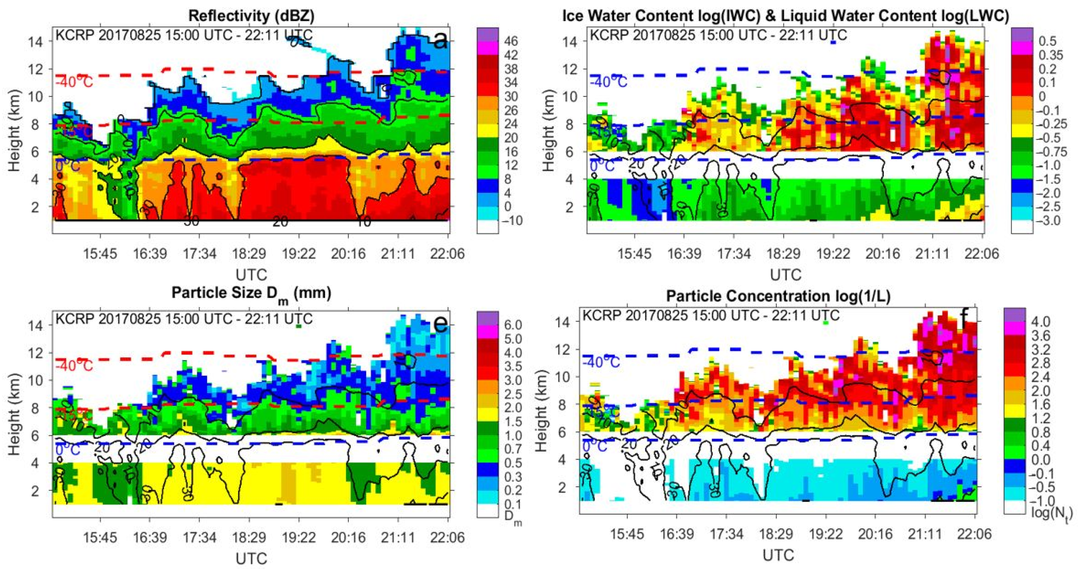
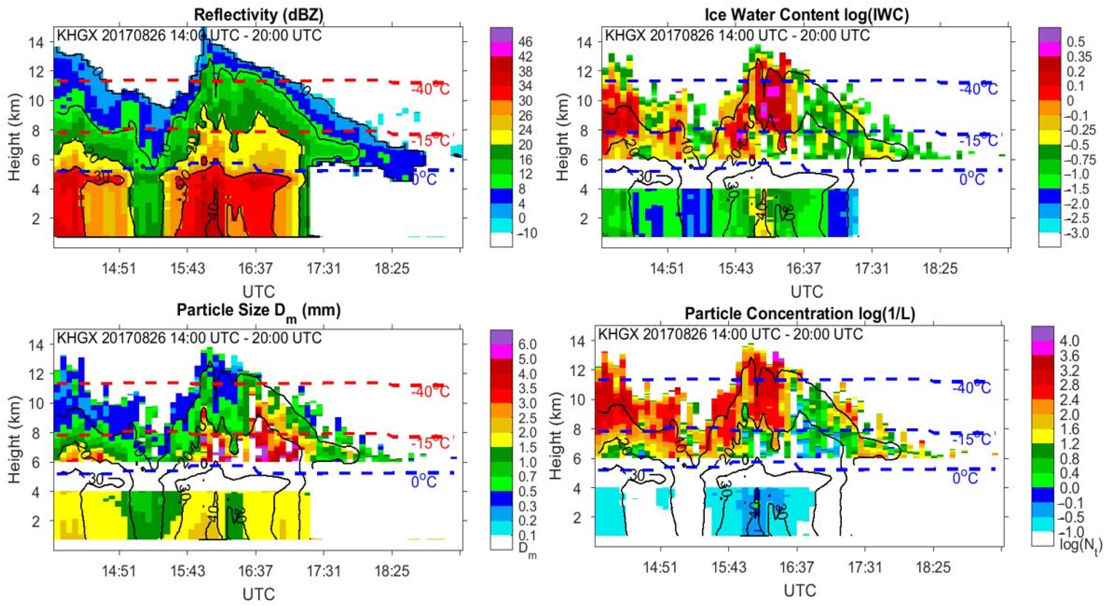
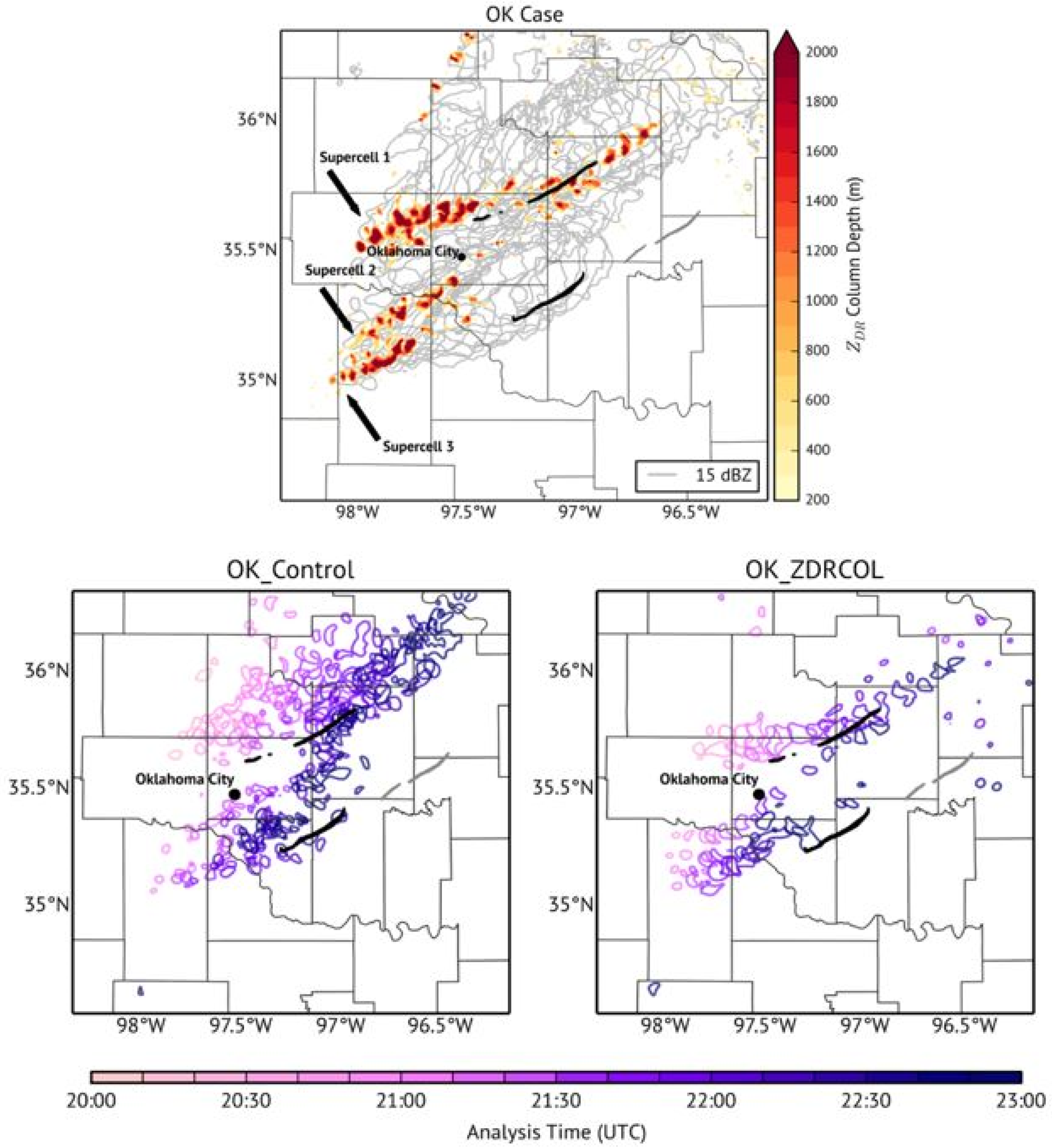
3.3. Illustration of the Polarimetric Microphysical Retrievals for Hurricane Harvey

Polarimetric microphysical retrievals in rain and ice have been used to investigate the microphysical structure of Hurricane Harvey (2017) as it made landfall on the Texas coast on 25 August 2017. The eyewalls of hurricanes and their outer rain bands have very different microphysical characteristics and the potential for flash flooding. Hurricane Harvey exemplifies this difference well. The composite vertical profiles of LWC/IWC, Dm, and Nt retrieved from columnar vertical profiles (CVP) (Murphy et al. [106]) of polarimetric radar variables have been generated in the eyewall area of the hurricane and its outer rain bands (Hu et al. [107]). The centers of the CVP columns are shown in the PPIs of ZH in Figure 15. The eyewall region was better sampled by the KCRP WSR-88D radar in Corpus Christi (left panel in Figure 15), whereas the outer rain band was better visible from the perspective of the KHGX WSR-88D radar in Houston (right panel in Figure 15). The corresponding CVPs in a height versus time format are shown in Figure 16 and Figure 17.
A comparison of the two CVPs in Figure 16 and Figure 17 indicates that the eyewall region and its periphery marked by the white box in the left panel of Figure 15 is characterized by a high concentration of very small ice particles aloft with ZH generally less than 20 dBZ above the melting layer. Vertical gradients of Z, LWC, and Dm are obviously higher in rain below the melting layer in the eyewall area than in the outer rain bands, which tells that the bulk of precipitation in the eyewall is formed as “warm” rain, and ice aloft makes a relatively small contribution to the rainfall at the surface, although the IWC aloft is high. It is the warm rain mechanism that is primarily responsible for precipitation in the eyewall.
The outer rain band is characterized by noticeably higher ZH in ice above the melting layer, larger ice particles, and lower Nt. The relative contribution of “warm” rain to the surface precipitation is lower, because vertical gradients of the polarimetric variables, IWC, and Dm are smaller compared to the eyewall region. Figure 17 shows that the LWC even decreases from the melting layer down to the surface. This means that a good portion of precipitation at the surface is from the melting of ice. The coexistence of graupel-size ice, ice crystals, and supercooled water lofted in stronger updrafts facilitates electric charge separation and significant lightning discharges in the outer rain band. In contrast, no lightning was reported in the eyewall region of Hurricane Harvey.
The combination of warm rain generated below the melting layer and rain resulting from the melting of ice originating in stronger convective updrafts makes an outer rain band of tropical cyclones more efficient at producing heavy rain compared to the eyewall. Extremely heavy rain from the stalled external rain bands was responsible for most of the flooding during Harvey.

4. Thermodynamic Retrievals

Hydrometeors undergoing a phase transition exchange latent heat with the environment, and these diabatic processes are a fundamental driver of atmospheric motion across a range of spatial and temporal scales. Condensation of water vapor in convective updrafts releases latent heat and drives convection through increases in buoyancy. Riming/accretion and refreezing represent another source of latent heat release that warms the environment. Evaporation and sublimation cool and moisten the environment, whereas the depositional growth of ice results in warming and drying. Melting of hydrometeors also causes cooling of the environment and, combined with evaporation and precipitation loading, may produce strong downdrafts associated with “cold pools” and microbursts. Polarimetric radar variables are very sensitive to the phase transitions of hydrometeors and, thus, can be very useful for thermodynamic retrievals in addition to the microphysical retrievals described in the previous section.
Carlin et al. [108] and Carlin and Ryzhkov [87] suggested a new paradigm of using polarimetric radar data for thermodynamic retrievals of warming and cooling rates associated with latent heat release and absorption. The rate of change of the environmental temperature due to latent heating can be described by (Grim et al. [109]):
d T d t = 1 c p ρ a { L s d m i , s u b l ( D ) d t N ( D ) d D + L v d m w , e v a p ( D ) d t N ( D ) d D + L f k a ( T T p ) d Q d m i , m e l t ( D ) d t N ( D ) d D }
where N(D) is the size distribution of mixed-phase particles; dmi,subl/dt and dmi,melt/dt are the rates of ice loss due to sublimation and melting; dmw,evap/dt is the rate of water mass loss due to evaporation; and Ls, Lv, and Lf are latent heat of sublimation, vaporization, and fusion. A similar equation can be written for the rate of change of the environmental water vapor mixing ratio qv:
d q v d t = 1 ρ a , d [ d m i , s u b l ( D ) d t + d m w , e v a p ( D ) d t ] N ( D ) d D
In Equations (17)–(18), T is the air temperature, Tp is the temperature of the particle, cp is the specific heat of the air, ρa is the air density, ρa,d is the dry air density, ka is the thermal diffusivity of air, and dQ is the heat available for melting. The rates dm/dt are determined by environmental thermodynamic variables, whereas the size distributions of pure rain and pure ice can be retrieved from polarimetric radar measurements using Equations (6)–(14) and assuming μ = 0. These can be used directly to estimate the warming/cooling rates dT/dt and moistening/drying rates dqv/dt using Equations (17) and (18). Conceptually, if reliable SD retrievals from radar measurements are not possible through the full depth of the cloud (e.g., due to a muted polarimetric signature in regions of intense aggregation), SDs obtained in regions of reliable retrievals can instead be used to initialize 1D Lagrangian cloud models to evolve the SD in less-reliable regions. An example of such an approach is the analytical model of depositional growth and the aggregation of snowflakes of Passarelli [110] and Mitchell [111], which requires an initial intercept and slope parameter of the particle size distributions to evolve downward that could be derived from radar. In practice, quantifying the uncertainty of the SD profile obtained this way will require estimates of the uncertainty associated with both the initial SD retrieved from radar and the model used to evolve the SD downward, which should be a focus of future studies.
Diabatic warming due to the condensation of water vapor in convective updrafts is a primary driving force of deep convection. Unfortunately, it is hard to capture the condensation process directly with a radar because of the very small size of cloud water droplets, which are usually invisible to the radar at commonly used precipitation radar wavelengths. However, warming due to condensation in deep moist convections can be better quantified with polarimetric radar markers, such as ZDR column height, compared to more commonly used metrics such as ZH or the rain rate (also estimated from ZH). Such an approach is exemplified by (though not limited to) the so-called “SLH” latent heating retrieval method described in Shige et al. [112,113]. In these approaches, convection-resolving models are coupled to radar operators to calculate reflectivity and run over a long period of time to generate a lookup table of mean vertical profiles of latent heating indexed by a radar observable such as a 10-dBZ height (e.g., see Figure 5 of [112]). These tables are then used to derive the vertical profiles of latent heating from observed reflectivity data. Such lookup table approaches have proved popular and continue to be developed and refined (e.g., Ahmed et al. [114]).
Our simulations of deep convective storms using the HUCM coupled with a polarimetric forward radar operator show that using the height of the 1-dB ZDR surface above the freezing level is a much better index of the vertical warming/cooling profiles than any Z-related parameter. This is illustrated in Figure 18, where these profiles are displayed as functions of the height of the 10-dBZ surface of ZH and 1-dB surface of ZDR in a deep hail-bearing convective storm (top panels a and b). It is obvious that the vertical cross-section of latent heating retrieved using the ZDR-based index (panel e) is in much better agreement with the “true” modeled distribution of latent heating (panel c) than the one retrieved using the ZH-based index (panel d). While the exact values of heating simulated in the lookup table shown in Figure 18b are expected to be somewhat sensitive to the model parameters used in the simulation (e.g., the environment, CCN, etc.), the correspondence between the latent-heating rate and ZDR column height overall appears robust and is in agreement with the results presented in Figure 6, as the latent-heating rate and w are inherently related.
Carlin et al. [108] demonstrated that the use of ZDR columns as proxies for convective updrafts has apparent advantages for radar data assimilation compared to the traditional utilization of ZH. One common technique of reflectivity data assimilation is using a cloud analysis, which inserts temperature and moisture increments, as well as hydrometeors deduced from ZH via empirical relations, to induce and sustain updraft circulations. In the study of Carlin et al. [108], the advanced regional prediction system’s (ARPS) cloud analysis was modified from its original ZH-based formulation to provide moisture and latent heat adjustments based on ZDR columns. In this approach, observed ZDR columns are used to isolate where positive temperature and moisture perturbations are applied, and modest amounts of moisture are removed outside of these locations if/at/or near saturation.
In the top panel of Figure 19, 15-dBZ contours of ZH (in grey) and color-shaded (ZDR) column depths between 2000 and 2300 UTC are displayed in 10-min intervals for the 19 May 2013 tornadic supercells in Oklahoma. In the two bottom panels of Figure 19, the ARPS model runs after assimilation of the ZH data only (single-pol run, left bottom panel), and the ZDR column information (dual-pol run, right bottom panel) are compared. The analyzed updraft tracks in the dual-pol run are more coherent and consolidated, with less spurious convection than in the single-pol run. The short-term forecast according to the dual-pol run shows a reduction in forward speed and northward position bias of the main updrafts, an issue encountered in many storm-scale modeling experiments. These results suggest that polarimetric radar data can provide more targeted increments of heating with positive forecast impacts.
In the melting layer and below, cooling due to the melting and evaporation of hydrometeors usually occurs. These cooling rates can be quantified using simplified 1D Lagrangian models with spectral bin microphysics coupled with a PRFO. In our analyses, we utilized 1D Lagrangian models for melting hail (Ryzhkov et al. [22]) and melting snow (Carlin and Ryzhkov [87]) and the PRFO of Ryzhkov et al. [15].
A typical vertical profile of the simulated cooling rate from our 1D model [22] below the freezing level for a hailstorm is shown in Figure 20 (right panel). This model includes melting, the soaking of meltwater into graupel and hailstones with densities less than that of solid ice, the spontaneous breakup of raindrops greater than 8 mm, and the shedding of meltwater into raindrops according to Rasmussen and Heymsfield [115]. In addition to the aforementioned processes described in [22], the sublimation of dry hail and evaporation of meltwater and shed water are included. The PRFO utilized T-matrix scattering computations and followed all assumptions for melting hail and graupel described in [15], including varying σα as a linear function of fw and the aspect ratio during melting according to [115]. Since this spectral model explicitly and separately treats the melting and evaporation of graupel, hail, and rain, their relative contributions to the cooling rate can be estimated (left panel in Figure 20). As expected, the sublimation and melting of graupel are the dominant contributors to the cooling rate within the first kilometer beneath the melting level, whereas the melting of hail and evaporation of raindrops dominate the cooling rate below, with the evaporation of raindrops originating from the complete melting of graupel and hail particles, making the largest contribution near the surface. Combining these results with the radar operator [15], it can be shown that the vertical gradient of KDP is well-correlated with the intensity of diabatic cooling in the first two km below the freezing level.
The methodology for estimating cooling rates due to rain evaporation using a 1D spectral bin model and the data collected by dual-polarization radar and micro-rain radar has been developed and demonstrated in Xie et al. [116]. It was shown that polarimetric radar observations can be used to estimate the evaporative cooling rates from the retrieved DSD aloft and the evaporation model.
Carlin and Ryzhkov [87] showed through simulations that the maximal cooling rates in the melting layer (ML) of stratiform precipitation can be determined from the maximal value of KDP within the ML. This is well-illustrated in Figure 21. The scatterplots of maximal cooling rates versus maximal ZH show tremendous variability caused by the diversity of size distributions of ice aloft and changes of vertical profiles of temperature and humidity within the ML (top panels in Figure 21), whereas the almost perfect linear dependencies of the max(dT/dt) on max(KDP) (bottom panels in Figure 21) show great promise. The reason for the strong correlation between the cooling rates and KDP is that both parameters are dominated by contributions from smaller particles in the size spectrum within the melting layer, whereas Z is heavily weighted by a few large melting snowflakes. Carlin and Ryzhkov [87] show that the cooling rate due to melting is proportional to the moment of the order 1.3 of the size distribution, whereas KDP is proportional to the moment of the order 1.1.

5. Conclusions

This paper provides an overview of several benefits that polarimetric weather radar may provide to the cloud-modeling community in an effort to improve the performance of numerical weather prediction (NWP) models and the microphysical parameterizations that they use. Polarimetric weather radar data can be leveraged by NWP models with the use of microphysical and thermodynamic retrievals or a polarimetric radar forward operator (PRFO). The retrieval concept essentially converts radar information into quantities that the model prognoses, such as liquid or ice water content, particle mean volume diameter, and number concentration, as well as the warming/cooling and moistening/drying rates. The PRFO path converts the model output into polarimetric radar fields for direct comparison with the radar observations.
A brief review of existing PRFOs is provided, with a list of necessary formulas for computing polarimetric radar variables from the model outputs presented in the Appendix A. The use of PRFOs with models employing spectral bin microphysics is relatively straightforward, whereas coupling the PRFOs with models that use bulk microphysical parameterization requires certain adaptations, such as the generation of artificial mixed-phase hydrometeor categories that are typically not produced in bulk schemes.
The techniques for microphysical polarimetric retrievals in rain are relatively well-established, as opposed to the retrievals in snow, which were introduced only recently. The retrieval equations for ice/snow have been derived assuming an inverse dependence of particle density on the equivolume diameter. Therefore, they cannot be used in areas dominated by graupel or hail. The ice microphysical retrievals heavily rely on the reliable estimation of the specific differential phase (KDP), which may require substantial spatial averaging.
Thermodynamic radar retrievals are a new frontier of research and show good promise, as the areas of the phase transition of water, such as vapor condensation or snow melting, are usually associated with pronounced polarimetric radar signatures. The way to quantify the rates of diabatic warming/cooling and moistening/drying using polarimetric radar data is outlined in the article and illustrated by a couple of examples.
This study describes several modifications in the HUCM, such as enabling the model to reproduce realistic ZDR columns in the simulations, that result from the partnership between cloud modelers at the Hebrew University of Jerusalem and radar meteorologists at the University of Oklahoma and the National Severe Storms Laboratory. Such partnerships can be considered as a model to facilitate the use of polarimetric weather radars for optimizing the performance of NWP models in a future.

Author Contributions

A.V.R. and A.K. provided conceptualization, project administration, and supervision; A.V.R. wrote the original draft, and J.S. and J.T.C. did the review and editing; J.S. and M.P. developed the software for the forward operator and coupled it with the HUCM cloud model; and J.T.C. conducted research on the radar thermodynamic retrievals. All authors have read and agreed to the published version of the manuscript.

Funding

Funding was provided by the NOAA/Office of Oceanic and Atmospheric Research under the NOAA-University of Oklahoma Cooperative Agreement #NA16OAR4320115, U.S. Department of Commerce, by the US Department of Energy ASR program under grants DE-SC0008811, DE-SC0014295, and DE-SC0018967. Additional support came from the US-Israeli Binational Science Foundation.

Acknowledgments

The authors are grateful to Jiaxi Hu for generating Figure 15, Figure 16 and Figure 17 of the manuscript.

Conflicts of Interest

The authors declare no conflicts of interest.

Appendix A

Expressions for polarimetric radar variables used in forward radar operators
Following Ryzhkov et al. [15], the radar variables can be computed from the output of NWP models using average backward and forward-scattering amplitudes per unit volume and angular moments characterizing the orientations of hydrometeors as follows:
Z h = 4 λ 4 π 5 | K w | 2 { < | s b ( π ) | 2 > 2 Re < [ s b ( π ) * ( s b ( π ) s a ( π ) ) ] > A 2 + < | s b ( π ) s a ( π ) | 2 > A 4 }
Z v = 4 λ 4 π 5 | K w | 2 { < | s b ( π ) | 2 > 2 Re < [ s b ( π ) * ( s b ( π ) s a ( π ) ) ] > A 1 + < | s b ( π ) s a ( π ) | 2 > A 3 }
Z d r = Z h Z v
L d r = 4 λ 4 π 4 | K w | 2 < | s b ( π ) s a ( π ) | 2 > A 5 Z h
K D P = 0.18 λ π < Re ( s b ( 0 ) s a ( 0 ) ) > ( A 1 A 2 )
ρ h v = 4 λ 4 π 4 | K w | 2 | < | s b ( π ) | 2 > + < | s b ( π ) s a ( π ) | 2 > A 5 < s b ( π ) * ( s b ( π ) s a ( π ) ) > A 1 < s b ( π ) ( s b ( π ) * s a ( π ) * ) > A 2 | ( Z h Z v ) 1 / 2
A h = 8.686 λ Im [ < s b ( 0 ) > < ( s b ( 0 ) s a ( 0 ) ) > A 2 ]
A D P = 8.686 λ Im ( < s b ( 0 ) > < s a ( 0 ) > ) ( A 1 A 2 )
where angular brackets indicate integration over particle size distribution N(D), e.g.,
< | s b ( π ) | 2 > = | s b ( π ) ( D ) | 2 N ( D ) d D
The scattering amplitudes s a , b ( π , 0 ) are computed either using the Rayleigh formulas for uniformly filled and two-layer spheroids or numerical methods such as the T-matrix or others.
In (A1)–(A8), Z h , v = 10 0.1 Z H , V ( d B Z ) , Z d r = 10 0.1 Z D R ( d B ) , L d r = 10 0.1 L D R ( d B ) , and Kw = (εw − 1)/(εw + 2), where εw is the dielectric constant of water, and radar wavelength λ and scattering amplitudes sa,b are expressed in mm, Zh,v are in mm6m−3, KDP is in deg km−1, and Ah and ADP are in dB km−1. Angular moments are defined as
A 1 = < sin 2 ψ cos 2 α > , A 2 = < sin 2 ψ sin 2 α > , A 3 = < sin 4 ψ cos 4 α > , A 4 = < sin 4 ψ sin 4 α > , A 5 = < sin 4 ψ cos 2 α sin 2 α > .
The expressions for the angular moments for different particle orientation types can be found in Ryzhkov [9] and Ryzhkov and Zrnic [3] (their section 3.4 and Appendix B).
Attenuation effects are taken into account by using equations
Z h ˜ = Z h 10 0.2 A h ( s ) d s
Z d r ˜ = Z d r 10 0.2 A D P ( s ) d s
L d r ˜ = L d r 10 0.1 A D P ( s ) d s
where a tilde overbar denotes the radar variables affected by attenuation/differential attenuation.

References

  1. Bringi, V.; Chandrasekar, V. Polarimetric Doppler Weather Radar. Principles and Applications; Cambridge University Press: Cambridge, UK, 2001; p. 634. [Google Scholar]
  2. Zhang, G. Weather Radar Polarimetry; CRC Press: Boca Raton, FL, USA, 2016; p. 304. [Google Scholar]
  3. Ryzhkov, A.; Zrnic, D. Radar Polarimetry for Weather Observations; Springer Atmospheric Sciences: Cham, Switzerland, 2019; p. 486. [Google Scholar]
  4. Morrison, H.; Milbrandt, J.; Bryan, G.; Ikeda, S.; Tessendorf, S.; Thompson, G. Parameterization of Cloud Microphysics Based on the Prediction of Bulk Ice Particle Properties. Part II: Case Study Comparisons with Observations and Other Schemes. J. Atmos. Sci. 2015, 72, 312–339. [Google Scholar] [CrossRef]
  5. Fan, J.; Han, B.; Varble, A.; Morrison, H.; North, K.; Kollias, P.; Chen, B.; Dong, X.; Giangrande, S.E.; Khain, A.; et al. Cloud-resolving model intercomparisons of an MC3E squall line case: Part I—Convective updrafts. J. Geophys. Res. Atmos. 2017, 122, 9351–9378. [Google Scholar] [CrossRef]
  6. Melnikov, V.; Zrnic, D.; Doviak, R.; Chilson, P.; Mechem, D.; Kogan, Y. Prospects of the WSR-88D radar for cloud studies. J. Appl. Meteorol. Climtol. 2011, 50, 859–872. [Google Scholar] [CrossRef] [Green Version]
  7. Zhang, G.; Mahale, V.N.; Putnam, B.J.; Qi, Y.; Cao, Q.; Byrd, A.D.; Bukovcic, P.; Zrnic, D.S.; Gao, J.; Xue, M.; et al. Current status and future challenges of weather radar polarimetry: Bridging the gap between radar meteorology/hydrology/engineering and numerical weather prediction. Adv. Atmos. Sci. 2019, 36, 571–588. [Google Scholar] [CrossRef] [Green Version]
  8. Holt, A. Some factors affecting the remote sensing of rain by polarization diversity radar in the 3- to 35-GHz frequency range. Radio Sci. 1984, 19, 1399–1412. [Google Scholar] [CrossRef]
  9. Ryzhkov, A. Interpretation of polarimetric radar covariance matrix for meteorological scatterers. Theoretical analysis. J. Atmos. Ocean. Technol. 2001, 18, 315–328. [Google Scholar] [CrossRef]
  10. Holt, A.; Shepherd, J. Electromagnetic scattering by dielectric spheroids in the forward and backward directions. J. Phys. A Math. General 1979, 12, 159–166. [Google Scholar] [CrossRef]
  11. Vivekanandan, J.; Adams, W.; Bringi, V. Rigorous approach to polarimetric radar modeling of hydrometeor orientation distributions. J. Appl. Meteorol. 1991, 30, 1053–1063. [Google Scholar] [CrossRef] [Green Version]
  12. Van de Hulst, H. Light Scattering by Small Particles; Dover: New York, NY, USA, 1981; p. 536. [Google Scholar]
  13. Maxwell Garnett, J. Color in metal glasses and in metallic films. Philos. Trans. R. Soc. Lond. A 1904, 203, 385–420. [Google Scholar]
  14. Bohren, C.; Huffman, D. Absorption and Scattering of Light by Small Particles; Wiley: Hoboken, NJ, USA, 1983; p. 530. [Google Scholar]
  15. Ryzhkov, A.; Pinsky, M.; Pokrovsky, A.; Khain, A. Polarimetric radar observation operator for a cloud model with spectral microphysics. J. Appl. Meteorol. Climatol. 2011, 50, 873–894. [Google Scholar] [CrossRef]
  16. Waterman, P. Matrix formulation of electromagnetic scattering. Proc. IEEE 1965, 53, 805–812. [Google Scholar] [CrossRef]
  17. Barber, P.; Yeh, C. Scattering of electromagnetic waves by arbitrary shaped dielectric bodies. Appl. Opt. 1975, 14, 2684–2872. [Google Scholar] [CrossRef] [PubMed]
  18. Mishchenko, M. Calculation of the amplitude matrix for a nonspherical particle in a fixed orientation. Appl. Opt. 2000, 39, 1026–1031. [Google Scholar] [CrossRef] [PubMed]
  19. Bringi, V.; Seliga, T. Scattering from axisymmetric dielectrics or perfect conductors imbedded in an axisymmetric dielectric. IEEE Trans. Antennas Prop. 1977, 25, 575–580. [Google Scholar] [CrossRef]
  20. Aydin, K.; Zhao, Y. A computational study of polarimetric radar observables in hail. IEEE Trans. Geosci. Remote Sens. 1990, 28, 412–422. [Google Scholar] [CrossRef]
  21. Depue, T.; Kennedy, P.; Rutledge, S. Performance of the hail differential reflectivity (HDR) polarimetric hail indicator. J. Appl. Meteorol. Climatol. 2007, 46, 1290–1301. [Google Scholar] [CrossRef] [Green Version]
  22. Ryzhkov, A.; Kumjian, M.; Ganson, S.; Khain, A. Polarimetric radar characteristics of melting hail. Pt I: Theoretical simulations using spectral microphysical modeling. J. Appl. Meteorol. Climatol. 2013, 52, 2849–2870. [Google Scholar] [CrossRef]
  23. Lu, Y.; Clothiaux, E.; Aydin, K.; Botta, G.; Verlinde, J. Modeling variability in dendritic ice crystal backscattering cross sections at millimeter wavelengths using a modified Rayleigh-Gans theory. J. Quant. Spectros. Radiat. Transfer 2013, 131, 95–104. [Google Scholar] [CrossRef]
  24. Aydin, K.; Seliga, T. Radar polarimetric backscattering properties of conical graupel. J. Atmos. Sci. 1984, 41, 1887–1892. [Google Scholar] [CrossRef] [Green Version]
  25. Waterman, P. Scattering by dielectric obstacles. Alta Freq. 1969, 38, 348–352. [Google Scholar]
  26. Lu, Y.; Jiang, Z.; Aydin, K.; Verlinde, J.; Clothiaux, E.; Botta, G. A polarimetric scattering database for non-spherical ice particles at microwave wavelengths. Atmos. Meas. Tech. 2016, 9, 5119–5134. [Google Scholar] [CrossRef] [Green Version]
  27. Xu, Y. Electromagnetic scattering by an aggregate of spheres. Appl. Opt. 1995, 34, 4573–4588. [Google Scholar] [CrossRef] [PubMed]
  28. Yurkin, M.; Hoekstra, A. The discrete-dipole approximation code ADDA: Capabilities and known limitations. J. Quant. Spectros. Radiat. Transfer. 2011, 112, 2234–2247. [Google Scholar] [CrossRef]
  29. Mirkovic, D. Computational Electromagnetics for Polarimetric Radar Scatterers: An Approach to Polarimetric Variable Modeling of Hydrometeors and Biota; Lambert Academic Publishing: Saarbrucken, Germany, 2016; p. 272. [Google Scholar]
  30. Harrington, R. Field Computation by Moment Methods; IEEE PRESS Series on Electromagnetic Waves: Piscataway, NJ, USA, 1993; p. 228. [Google Scholar]
  31. WIPL-D. WIPL-D Pro EM Solver. (WIPL-D d.o.o). 2019. Available online: www.wipl-d.com (accessed on 15 January 2020).
  32. Botta, G.; Aydin, K.; Verlinde, J. Modeling of microwave scattering from cloud ice crystal aggregates and melting aggregates: A new approach. IEEE Geosci. Remote Sens. Lett. 2010, 7, 572–576. [Google Scholar] [CrossRef]
  33. Tyynela, J.; Leinonen, J.; Moisseev, D.; Nousiainen, T. Radar backscattering from snowflakes: Compariosn of fractal, aggregate, and soft spheroid models. J. Atmos. Ocean. Technol. 2011, 28, 1365–1372. [Google Scholar] [CrossRef] [Green Version]
  34. Leinonen, J.; Kneifel, S.; Moisseev, D.; Tyynela, J.; Tanelli, S.; Nousianen, T. Evidence of nonspheroidal behavior in millimeter-wavelength radar observations of snowfall. J. Geophys. Res. 2012, 117, D18205. [Google Scholar] [CrossRef]
  35. Tyynela, J.; Chandrasekar, V. 2014: Characterizing falling snow using multifrequency dual-polarization measurements. J. Geophys. Res. Atmos. 2014, 119, 8268–8283. [Google Scholar]
  36. Ori, D.; Maestri, T.; Rizzi, R.; Montopoli, M.; Marzano, F. Scattering properties of modeled complex snowflakes and mixed-phase particles at microwave and millimeter frequencies. J. Geophys. Res. Atmos. 2014, 119, 9931–9947. [Google Scholar] [CrossRef]
  37. Leinonen, J.; Moisseev, D. What do triple-frequency radar signatures reveal about aggregate snowflakes? J. Geophys. Res. Atmos. 2015, 120, 229–239. [Google Scholar] [CrossRef]
  38. Schrom, R.; Kumjian, M. Bulk-density representations of branched planar ice crystals: Errors in the polarimetric radar variables. J. Appl. Meteorol. Climatol. 2018, 57, 333–346. [Google Scholar] [CrossRef]
  39. Fabry, F.; Szyrmer, W. Modeling of the melting layer. Part II: Electromagnetic. J. Atmos. Sci. 1999, 56, 3593–3600. [Google Scholar] [CrossRef]
  40. Chobanyan, E.; Sekeljic, N.; Ilic, M.; Bringi, V.; Notaros, B. Efficient and accurate computational electromagnetics approach to precipitation particle scattering analysis based on higher-order method of moments integral equation modeling. J. Atmos. Ocean. Technol. 2015, 32, 1745–1758. [Google Scholar] [CrossRef]
  41. Milbrand, J.; Yau, M. A multimoment bulk microphysical parameterization. Part II: A proposed three-moment closure and scheme description. J. Atmos. Sci. 2005, 62, 3065–3081. [Google Scholar] [CrossRef]
  42. Harrington, J.; Sulia, K.; Morrison, H. A method for adaptive habit prediction in bulk microphysical models. Part I: Theoretical development. J. Atmos. Sci. 2013, 70, 349–364. [Google Scholar]
  43. Sulia, K.; Kumjian, M. Simulated polarimetric fields of ice vapor growth using the Adaptive Habit Model. Part I: Large-Eddy Simulations. Mon. Weather Rev. 2017, 145, 2281–2302. [Google Scholar] [CrossRef]
  44. Sulia, K.; Kumjian, M. Simulated polarimetric fields of ice vapor growth using the Adaptive Habit Model. Part II: A case study from the FROST experiment. Mon. Weather Rev. 2017, 145, 2303–2323. [Google Scholar] [CrossRef]
  45. Li, H.; Moisseev, D.; von Lerber, A. How does riming affect dual-polarization radar observations and snowflake shape? J. Geophys. Res. Atmos. 2018, 123, 6070–6081. [Google Scholar] [CrossRef]
  46. Matrosov, S.; Reinking, R.; Kropfli, R.; Bartram, B. Estimation of ice hydrometeor types and shapes from radar polarization measurements. J. Atmos. Ocean. Technol. 1996, 13, 85–96. [Google Scholar] [CrossRef] [Green Version]
  47. Straka, J.; Zrnic, D.; Ryzhkov, A. Bulk hydrometeor classification and quantification using multiparameter radar data. Synthesis of relations. J. Appl. Meteorol. 2000, 39, 1341–1372. [Google Scholar] [CrossRef]
  48. Korolev, A.; Isaac, G. Roundness and aspect ratio of particles in ice clouds. J. Atmos. Sci. 2003, 60, 1795–1808. [Google Scholar] [CrossRef]
  49. Matrosov, S.; Schmitt, C.; Maahn, M.; de Boer, G. Atmospheric ice particle shape estimates from polarimetric radar measurements and in situ observations. J. Atmos. Ocean. Technol. 2017, 34, 2569–2587. [Google Scholar] [CrossRef]
  50. Matrosov, S. Ice hydrometeor shape estimations using polarimetric operational and research radar measurements. Atmosphere 2020, 11, 97. [Google Scholar] [CrossRef] [Green Version]
  51. Jung, Y.; Zhang, G.; Xue, M. Assimilation of simulated polarimetric radar data for a convective storm using the Ensemble Kalman Filter. Part I: Observation operators for reflectivity and polarimetric variables. Mon. Weather Rev. 2008, 136, 2228–2245. [Google Scholar] [CrossRef]
  52. Brandes, E.; Zhang, G.; Vivekanandan, J. Experiments in rainfall estimation with polarimetric radar in a subtropical environment. J. Appl. Meteorol. 2002, 41, 674–685. [Google Scholar] [CrossRef] [Green Version]
  53. Melnikov, V.; Straka, J. Axis ratios and flutter angles of cloud ice particles: Retrievals from radar data. J. Atmos. Ocean. Technol. 2013, 30, 1691–1703. [Google Scholar] [CrossRef]
  54. Ryzhkov, A.; Bukovcic, P.; Murphy, A.; Zhang, P.; McFarquhar, G. Ice Microphysical Retrievals Using Polarimetric Radar Data. In Proceedings of the 10th European Conference on Radar in Meteorology and Hydrology, Ede, The Netherlands, 1–6 July 2018. [Google Scholar]
  55. Ray, P. Broadband complex refractive indices of ice and water. Appl. Opt. 1972, 11, 1836–1844. [Google Scholar] [CrossRef]
  56. Ryzhkov, A. The impact of beam broadening on the quality of radar polarimetric data. J. Atmos. Ocean. Technol. 2007, 24, 729–744. [Google Scholar] [CrossRef]
  57. Ryzhkov, A.; Zrnic, D. Depolarization in ice crystals and its effect on radar polarimetric measurements. J. Atmos. Ocean. Technol. 2007, 24, 1256–1267. [Google Scholar] [CrossRef] [Green Version]
  58. Hubbert, J.; Ellis, S.; Chang, W.-Y.; Rutledge, S.; Dixon, M. Modeling and interpretation of S-band ice crystals depolarization signatures from data obtained by simultaneously transmitting horizontally and vertically polarized fields. J. Appl. Meteorol. Climatol. 2014, 53, 1659–1676. [Google Scholar] [CrossRef]
  59. Pfeifer, M.; Craig, G.; Hagen, M.; Keil, C. A polarimetric radar forward operator for model evaluation. J. Appl. Meteorol. Climatol. 2008, 47, 3203–3220. [Google Scholar] [CrossRef] [Green Version]
  60. Baldauf, M.; Seifert, A.; Forstner, J.; Majewski, D.; Raschendorfer, M.; Reinhardt, T. Operational convective-scale numerical weather prediction with the COSMO Model: Description and sensitivities. Mon. Weather Rev. 2011, 139, 3887–3905. [Google Scholar] [CrossRef]
  61. Andsager, K.; Beard, K.; Laird, N. Laboratory measurements of axis ratios for large drops. J. Atmos. Sci. 1999, 56, 2673–2683. [Google Scholar] [CrossRef]
  62. Ryzhkov, A.; Zrnic, D.; Hubbert, J.; Bringi, V.; Vivekanandan, J.; Brandes, E. Polarimetric radar observations and interpretation of co-cross-polar correlation coefficients. J. Atmos. Ocean. Technol. 2002, 19, 340–354. [Google Scholar] [CrossRef] [Green Version]
  63. Xue, M.; Wang, D.; Gao, J.; Brewster, K.; Droegemeier, K. The Advanced Regional Prediction System (ARPS), storm-scale numerical weather prediction and data assimilation. Meteorol. Atmos. Phys. 2003, 82, 139–170. [Google Scholar] [CrossRef]
  64. Dawson, D.; Mansell, E.; Jung, Y.; Wicker, L.; Kumjian, M.; Xue, M. Low-level ZDR signatures in supercell forward flanks: The role of size sorting and melting of hail. J. Atmos. Sci. 2014, 71, 276–299. [Google Scholar] [CrossRef]
  65. Snyder, J.; Bluestein, H.; Dawson, D.; Jung, Y. Simulations of polarimetric, X-band radar signatures in supercells. Part I: Description of experiment and simulated ρhv rings. J. Appl. Meteorol. Climatol. 2017, 56, 1977–1999. [Google Scholar] [CrossRef]
  66. Snyder, J.; Bluestein, H.; Dawson, D.; Jung, Y. Simulations of polarimetric, X-band radar signatures in supercells. Part II: ZDR columns and rings and KDP columns. J. Appl. Meteorol. Climatol. 2017, 56, 2001–2026. [Google Scholar] [CrossRef]
  67. Khain, A.; Pinsky, M. Physical Processes in Clouds and Cloud Modeling; Cambridge University Press: Cambridge, UK, 2018; p. 686. [Google Scholar]
  68. Augros, C.; Caumont, O.; Ducrocq, V.; Gaussiat, N.; Tabary, P. Comparisons between S-, C-, and X-band polarimetric radar observations and convective-scale simulations of the HyMex first special observing period. Q. J. R. Meteorol. Soc. 2016, 142, 347–362. [Google Scholar] [CrossRef]
  69. Wolfensberger, D.; Berne, A. From model to radar variables: A new forward polarimetric radar operator for COSMO. Atmos. Meas. Tech. 2018, 11, 3883–3916. [Google Scholar] [CrossRef] [Green Version]
  70. Matsui, T.; Dolan, B.; Rutledge, S.; Tao, W.-K.; Iguchi, T.; Barnum, J.; Lang, S. POLARRIS: A POLArimetric Radar Retrieval and Instrument Simulator. J. Geophys. Res. Atmos. 2019, 124, 4634–4657. [Google Scholar] [CrossRef] [Green Version]
  71. Mendrok, J.; Snyder, J.; Troemel, S.; Blahak, U. Towards an Efficient Radar Forward Operator for NWP Frameworks. In Proceedings of the 39th Conference on Radar Meteorology, Nara, Japan, 16–20 September 2019. [Google Scholar]
  72. Oue, M.; Kollias, P.; Tatarevic, A.; Wang, D.; Yu, K. The Cloud Resolving Model Radar Simulator (CR-SIM) Version 3.3. 2019. Available online: https://commons.library.stonybrook.edu/somasdata/4 (accessed on 15 January 2020).
  73. Lafore, J.P.; Stein, J.; Asencio, N.; Bougeault, P.; Ducrocq, V.; Duron, J.; Fischer, C.; Héreil, P.; Mascart, P.; Masson, V.; et al. The Meso-NH Atmospheric Simulation System. Part I: Adiabatic formulation and control simulations. Ann. Geophys. 1998, 16, 90–106. [Google Scholar] [CrossRef]
  74. Zeng, Y.; Blahak, U.; Jerger, D. An efficient modular volume-scanning radar forward operator for NWP models: Description and coupling to the COSMO model. Q. J. R. Meteorol. Soc. 2016, 142, 3234–3256. [Google Scholar] [CrossRef]
  75. Kumjian, M.; Khain, A.; Benmoshe, N.; Ilotoviz, E.; Ryzhkov, A.; Phillips, V. The anatomy and physics of ZDR columns: Investigating a polarimetric radar signature with a spectral bin microphysical model. J. Appl. Meteorol. Climtol. 2014, 53, 1820–1843. [Google Scholar] [CrossRef]
  76. Snyder, J.; Ryzhkov, A.; Kumjian, M.; Khain, A.; Picca, J. A ZDR column detection algorithm to examine convective storm updrafts. Weather Forecast. 2015, 30, 1819–1844. [Google Scholar] [CrossRef]
  77. Ilotoviz, E.; Khain, A.; Ryzhkov, A.; Snyder, J. Relationship between aerosols, hail microphysics, and ZDR columns. J. Atmos. Sci. 2018, 75, 1755–1781. [Google Scholar] [CrossRef]
  78. Ortega, K.; Krause, J.; Ryzhkov, A. Polarimetric radar characteristics of melting hail. Part III: Validation of the algorithm for hail size discrimination. J. Appl. Meteorol. Climtol. 2016, 55, 829–848. [Google Scholar] [CrossRef]
  79. Kumjian, M.; Prat, O. The impact of raindrop collisional processes on the polarimetric radar variables. J. Atmos. Sci. 2014, 71, 3052–3067. [Google Scholar] [CrossRef]
  80. Prat, O.; Barros, A. Exploring the use of a column model for the characterization of microphysical processes in warm rain: Results from a homogeneous rainshaft model. Adv. Geosci. 2007, 10, 145–152. [Google Scholar] [CrossRef] [Green Version]
  81. Johnson, M.; Jung, Y.; Dawson, D.; Xue, M. Comparison of simulated polarimetric signatures in idealized supercell storms using two-moment bulk microphysics schemes in WRF. Mon. Weather Rev. 2016, 144, 971–996. [Google Scholar] [CrossRef]
  82. Johnson, M.; Jung, Y.; Dawson, D.; Supine, T.; Xue, M.; Park, J.; Lee, Y.-H. Evaluation of Unified Model microphysics in high-resolution NWP simulations using polarimetric radar observations. Adv. Atmos. Sci. 2018, 35, 771–784. [Google Scholar] [CrossRef] [Green Version]
  83. Kumjian, M.; Ryzhkov, A. Storm-relative helicity revealed from polarimetric radar measurements. J. Atmos. Sci. 2009, 66, 667–685. [Google Scholar] [CrossRef] [Green Version]
  84. Kumjian, M.; Ryzhkov, A. The impact of size sorting on the polarimetric radar variables. J. Atmos. Sci. 2012, 69, 2042–2060. [Google Scholar] [CrossRef]
  85. Kumjian, M.; Ryzhkov, A. The impact of evaporation on polarimetric characteristics of rain. Theoretical model and practical implications. J. Appl. Meteorol. Climatol. 2010, 49, 1247–1267. [Google Scholar] [CrossRef] [Green Version]
  86. Kumjian, M.; Ganson, S.; Ryzhkov, A. Freezing of raindrops in deep convective storms: A microphysical and polarimetric model. J. Atmos. Sci. 2012, 69, 3471–3490. [Google Scholar] [CrossRef]
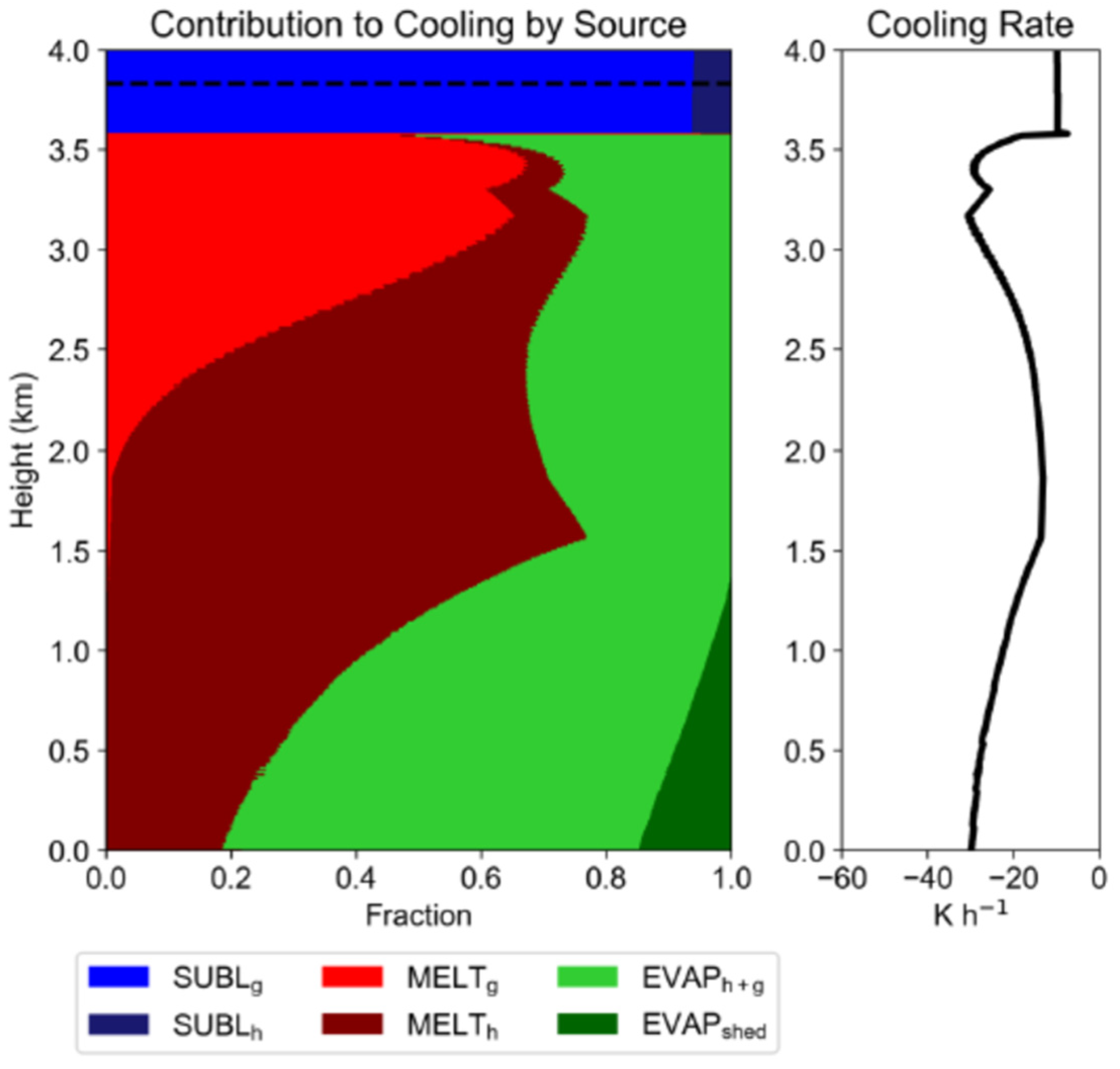
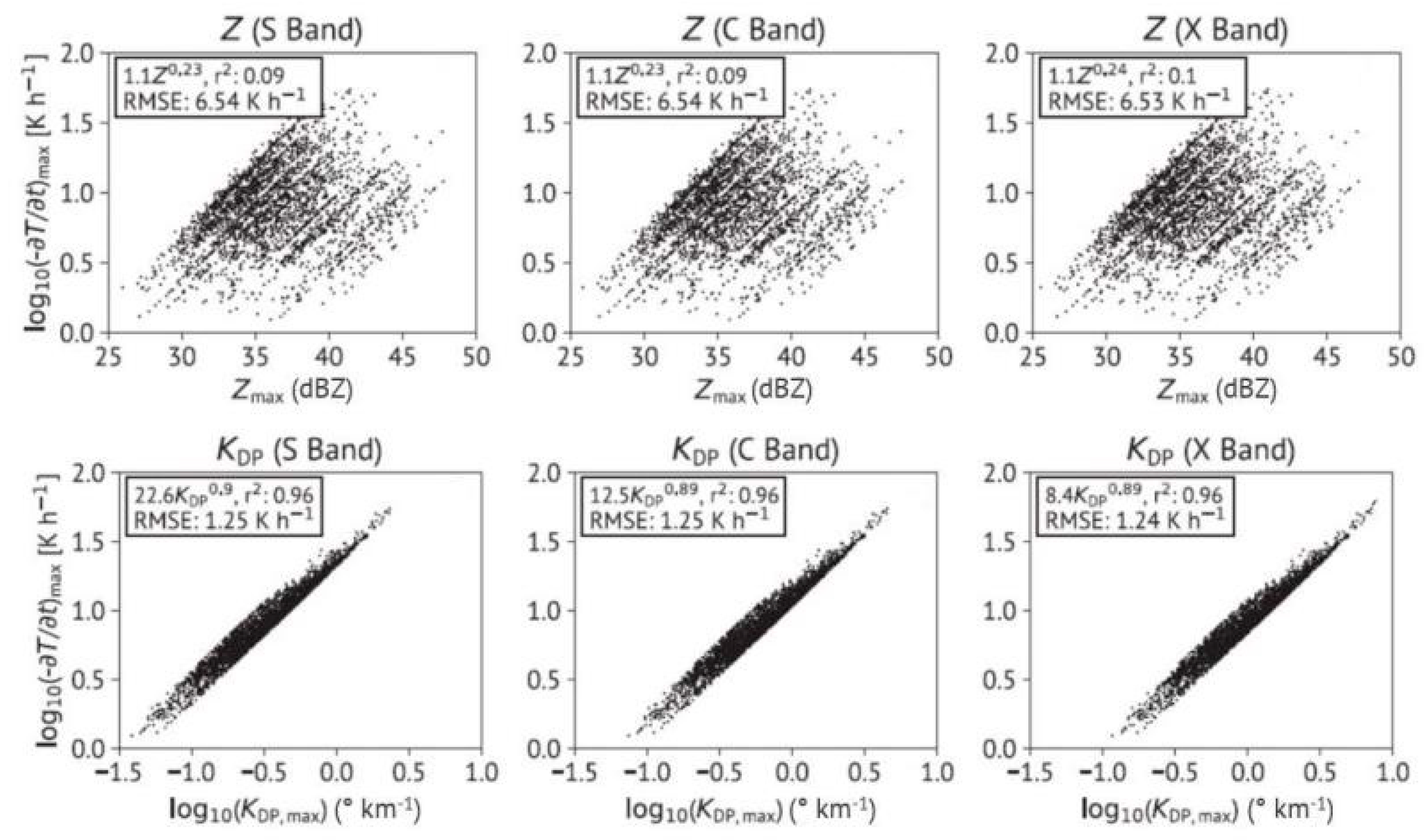
  87. Carlin, J.; Ryzhkov, A. Estimation of melting layer cooling rate from dual-polarization radar: Spectral bin model simulations. J. Appl. Meteorol. Climtol. 2019, 58, 1485–1508. [Google Scholar] [CrossRef]
  88. Jung, Y.; Xue, M.; Zhang, G. Simulations of polarimetric radar signatures of a supercell storm using a two-moment bulk microphysics scheme. J. Appl. Meteorol. Climtol. 2010, 49, 146–163. [Google Scholar] [CrossRef]
  89. Kumjian, M.; Ryzhkov, A. Polarimetric signatures in supercell storms. J. Appl. Meteorol. Climatol. 2008, 47, 1940–1961. [Google Scholar] [CrossRef]
  90. Ryzhkov, A.; Diederich, M.; Zhang, P.; Simmer, C. Utilization of specific attenuation for rainfall estimation, mitigation of partial beam blockage, and radar networking. J. Atmos. Ocean. Technol. 2014, 31, 599–619. [Google Scholar] [CrossRef]
  91. Wang, Y.; Cocks, S.; Tang, L.; Ryzhkov, A.; Zhang, P.; Zhang, J.; Howard, K. A prototype quantitative precipitation estimation algorithm for operational S-band polarimetric radar utilizing specific attenuation and specific differential phase: Part I–Algorithm description and initial results. J. Hydrometeorol. 2019, 20, 985–997. [Google Scholar] [CrossRef]
  92. Cocks, S.; Wang, Y.; Tang, L.; Ryzhkov, A.; Zhang, P.; Zhang, J.; Howard, K. A prototype quantitative precipitation estimation algorithm for operational S-band polarimetric radar utilizing specific attenuation and specific differential phase: Part II–Case study analysis and performance verification. J. Hydrometeorol. 2019, 20, 999–1014. [Google Scholar] [CrossRef]
  93. Zhang, J.; Tang, L.; Cocks, S.; Zhang, P.; Ryzhkov, A.; Howard, K.; Langston, C.; Kaney, B. A dual-polarization radar synthetic QPE for operations. J. Hydrometeorol. 2020. accepted. [Google Scholar] [CrossRef] [Green Version]
  94. Giangrande, S.; Ryzhkov, A. Estimation of rainfall based on the results of polarimetric echo classification. J. Appl. Meteorol. Climatol. 2008, 47, 2445–2462. [Google Scholar] [CrossRef]
  95. Zhang, J.; Howard, K.; Langston, C.; Kaney, B.; Qi, Y.; Tang, L.; Grams, H.; Wang, Y.; Cocks, S.; Martinaitis, S.; et al. Multi-Radar Multi-Sensor (MRMS) quantitative precipitation estimation: Initial operating capabilities. Bull. Am. Meteorol. Soc. 2016, 97, 621–638. [Google Scholar] [CrossRef]
  96. Brandes, E.; Zhang, G.; Vivekanandan, J. Drop size distribution retrieval with polarimetric radar: Model and application. J. Appl. Meteorol. 2004, 43, 461–475. [Google Scholar] [CrossRef] [Green Version]
  97. Cao, Q.; Zhang, G.; Brandes, E.; Schuur, T.; Ryzhkov, A.; Ikeda, K. Analysis of video disdrometer and polarimetric radar data to characterize rain microphysics in Oklahoma. J. Appl. Meteorol. Climtol. 2008, 47, 2238–2255. [Google Scholar] [CrossRef] [Green Version]
  98. Cao, Q.; Zhang, G.; Brandes, E.; Schuur, T. Polarimetric radar rain estimation through retrieval of drop size distribution using a Bayesian approach. J. Appl. Meteorol. Climatol. 2010, 49, 973–990. [Google Scholar] [CrossRef]
  99. Wen, G.; Chen, H.; Zhang, G.; Sun, J. An inverse model for raindrop size distribution retrieval with polarimetric variables. Remote Sens. 2018, 10, 1179. [Google Scholar] [CrossRef] [Green Version]
  100. Brandes, E.; Ikeda, K.; Zhang, G.; Schoenhuber, M.; Rasmussen, R. A statistical and physical description of hydrometeor distributions in Colorado snowstorms using a video-disdrometer. J. Appl. Meteorol. 2007, 46, 634–650. [Google Scholar] [CrossRef]
  101. Ryzhkov, A.; Zrnic, D.; Gordon, B. Polarimetric method for ice water content determination. J. Appl. Meteorol. 1998, 37, 125–134. [Google Scholar] [CrossRef]
  102. Hobbs, P.; Rangno, A. Ice particle concentrations in clouds. J. Atmos. Sci. 1985, 42, 2523–2549. [Google Scholar] [CrossRef] [Green Version]
  103. Nguyen, C.; Wolde, M.; Korolev, A. Determination of ice water content (IWC) in tropical convective clouds from X-band dual-polarization airborne radar. Atmos. Meas. Tech. 2019, 12, 5897–5911. [Google Scholar] [CrossRef] [Green Version]
  104. Griffin, E.; Schuur, T.; Ryzhkov, A. A polarimetric analysis of ice microphysical processes in snow, using quasi-vertical profiles. J. Appl. Meteorol. Climatol. 2018, 57, 31–50. [Google Scholar] [CrossRef]
  105. Carlin, J.; Ryzhkov, A.; Snyder, J.; Khain, A. Hydrometeor mixing ratio retrievals for strom-scale radar data assimilation: Utility of current equations and potential benefits of polarimetry. Mon. Weather Rev. 2016, 144, 2981–3001. [Google Scholar] [CrossRef]
  106. Murphy, A.; Ryzhkov, A.; Zhang, P. Columnar vertical profile (CVP) methodology for validating polarimetric radar retrievals in ice using in situ aircraft measurements. J. Atmos. Ocean. Technol. 2020. submitted. [Google Scholar]
  107. Hu, J.; Rosenfeld, D.; Ryzhkov, A.; Zhang, P. Synergetic use of the WSR-88D radars, GOES-R satellites, and lightning sensors to study microphysical characteristics of hurricanes. J. Appl. Meteorol. Climtol. 2019. accepted. [Google Scholar]
  108. Carlin, J.; Gao, J.; Snyder, J.; Ryzhkov, A. Assimilation of ZDR columns for improving the spin-up and forecast of convective storms in storm-scale models: Proof-of-concept experiments. Mon. Weather Rev. 2017, 145, 5033–5057. [Google Scholar] [CrossRef]
  109. Grim, J.; McFarquhar, G.; Rauber, R.; Smith, A.; Jewett, B. Microphysical and thermodynamic structure and evolution of the trailing stratiform regions of mesoscale convective systems during BAMEX. Part II: Column model simulations. Mon. Weather Rev. 2009, 137, 1186–1205. [Google Scholar] [CrossRef]
  110. Passarelli, R. An approximate analytical model of the vapor deposition and aggregation growth of snowflakes. J. Atmos. Sci. 1978, 35, 118–224. [Google Scholar] [CrossRef] [Green Version]
  111. Mitchell, D. Evolution of snow-size spectra in cyclonic storms. Part I: Snow growth by vapor deposition and aggregation. J. Atmos. Sci. 1988, 45, 3431–3451. [Google Scholar] [CrossRef] [Green Version]
  112. Shige, S.; Takayabu, N.; Tao, W.-K.; Johnson, D. Spectral retrieval of latent heating profiles from TRMM PR data. Part I: Development of a model-based algorithm. J. Appl. Meteorol. Climatol. 2004, 43, 1095–1113. [Google Scholar] [CrossRef]
  113. Shige, S.; Takayabu, N.; Tao, W.-K.; Johnson, D. Spectral retrieval of latent heating profiles from TRMM PR data. Part II: Algorithm improvement and heating estimates over tropical ocean regions. J. Appl. Meteorol. Climatol. 2007, 46, 1098–1124. [Google Scholar] [CrossRef]
  114. Ahmed, F.; Schumacher, C.; Feng, Z.; Hagos, S. A retrieval of tropical latent heating using the 3D structure of precipitation features. J. Appl. Meteorol. Climatol. 2016, 55, 1965–1982. [Google Scholar] [CrossRef]
  115. Rasmussen, R.M.; Heymsfield, A.J. Melting and shedding of graupel and hail. Part I: Model physics. J. Atmos. Sci. 1987, 44, 2754–2763. [Google Scholar] [CrossRef] [Green Version]
  116. Xie, X.; Evaristo, R.; Troemel, S.; Saavedra, P.; Simmer, C.; Ryzhkov, A. Radar observation of evaporation and implications for quantitative precipitation and cooling rate estimation. J. Atmos. Ocean. Technol. 2016, 33, 1779–1792. [Google Scholar] [CrossRef]
Figure 1. Scattering geometry. Direction N denotes the orientation of the symmetry axis of the particle, and k represents the direction of wave propagation (which is perpendicular to the polarization plane and lies in the x, z plane). The polarization plane is depicted by the grey ellipse. The x axis is true vertical, and y and z are the orthogonal horizontal directions. The canting angle α is the angle between the projections of vector N and true vertical x on the polarization plane, ψ is the angle between N and k, and the antenna elevation is β.
Atmosphere 11 00362 g001
Figure 2. Composite Range-Height Indicator (RHI) of Z and ZDR measured in a tornadic storm in Oklahoma on 29 May 2004. Overlaid are Z contours drawn every 5 dBZ.
Atmosphere 11 00362 g002
Figure 3. Fields of (left) simulated and (right) observed (top) Z and (bottom) ZDR in the vertical cross-section of an Oklahoma hailstorm on 2 February 2009 at the moment of its maximal development. Overlaid are 40- and 50-dBZ reflectivity contours. The white oval in the bottom right panel encloses the observed ZDR column. Note that the horizontal distances in the model and radar coordinates are different. From Ryzhkov et al. [15].
Atmosphere 11 00362 g003
Figure 4. Evolution of vertical cross-sections of ZH (left panels) and ZDR (right panels) throughout the life cycle of a hailstorm simulated using the Hebrew University cloud model (HUCM). Vertical velocity values of 10 m s−1 and 30 m s−1 are contoured in black, and the time within the simulation is in the upper-left corner of each panel. The polarimetric emulator used to produce these images is described in Ryzhkov et al. [15]. White letters “A”, “B”, and “C” highlight three ZDR columns. From Ryzhkov and Zrnic [3]. Used with permission from Springer.
Atmosphere 11 00362 g004
Figure 5. Cumulative histograms of ZDR column height (left) observed during Oklahoma tornadic storms on 19 May 2013 and (right) from an idealized storm simulated by the HUCM.
Atmosphere 11 00362 g005
Figure 6. Scatterplots of the 1-dB ZDR contour height above the 0 °C level (km) versus the updraft speed (m s−1) at that height. Different concentrations of CCN are marked by different colors: blue—100 cm−3, green—400 cm−3, brown—1000 cm−3, red—2000 cm−3, and black—3000 cm−3. Adapted from Ilotoviz et al. [77]. Used with permission from American Meteorological Society.
Atmosphere 11 00362 g006
Figure 7. Fields of (top) Z and (bottom) ZDR at the C band in a hailstorm simulated with (left) and without (right) spontaneous raindrop breakup. Adapted from Ilotoviz et al. [77].
Atmosphere 11 00362 g007
Figure 8. Distributions of Z and ZDR at different height intervals for different surface hail size categories from the HUCM (left panels) and radar observations (right panels). The short, thick vertical lines mark the median values of the distributions. The left and right boundaries of the colored boxes correspond to the 25th and 75th percentiles of the distributions. Radar variables are calculated at the S band. The definition of height intervals/classes is in [77,78]. From Ilotoviz et al. [77]. Used with permission from American Meteorological Society.
Atmosphere 11 00362 g008
Figure 9. (Left panel) Schematic of the two-dimensional wind shear model configuration: (left) storm-relative wind profile and (right) the domain and resulting Z distribution (shaded; dBZ). The “cloud” rainwater mixing ratio q (g/kg) profile is shown above the domain. (Right panels) Results from the two-dimensional wind shear model using the bin formulation: panels show the 2D fields of (a) ZH, (b) ZDR, (c) KDP, and (d) ρhv. Overlaid on (a) are the ZDR contours (0.5–2.5 dB in 0.5-dB increments); (b)–(d) have Z contours (10–40 dBZ in 10-dBZ increments) overlaid. Adapted from Kumjian and Ryzhkov [84].
Atmosphere 11 00362 g009
Figure 10. RHI scan of Z and ZDR taken at 0404 UTC 22 June 2011 from the Bonn X-band polarimetric radar. Adapted from Kumjian and Ryzhkov [84]. Used with permission from American Meteorological Society.
Atmosphere 11 00362 g010
Figure 11. The ρhv and ZDR rings simulated in a supercell storm at ~4.6 km above ground level (AGL), as shown by (a) ρhv (colors) and w (contoured every 10 m s−1), (b) Z (dBZ; colors) and ZDR (dB; contoured every 1 dB), and (c) a typical midlevel ρhv ring observed in the supercell. The polarimetric variables are calculated for the X band. Adapted from Snyder et al. [65,66] and Kumjian and Ryzhkov [89]. Used with permission from American Meteorological Society.
Atmosphere 11 00362 g011
Figure 12. Observed (left panels a,c) and simulated (right panels b,d) fields of Z and ZDR near the surface of the 1 June 2008 Oklahoma nontornadic supercell. Overlaid are the reflectivity contours in 20-dBZ increments. The ZDR arc in the southern part of the forward flank downdraft is enclosed in the black oval. Adapted from Dawson et al. [64]. Used with permission from American Meteorological Society.
Atmosphere 11 00362 g012
Figure 13. Scatterplots of the liquid water content (LWC) measured by the 2D video disdrometer in Oklahoma versus its estimates from (a) LWC(Z), (b) LWC(Z,ZDR), and (c) LWC(A) radar relations.
Atmosphere 11 00362 g013
Figure 14. Dependence of the mean volume diameter (Dm) of ice particles on [ZDP/(KDPλ)]1/2 for 12 various ice habits for exponential size distribution (µ = 0) and the factor α in (15) equal to 0.2. From Ryzhkov and Zrnic [3]. Used with permission from Springer.
Atmosphere 11 00362 g014
Figure 15. Plan position indicator (PPI) images of ZH at a 0.5° elevation angle. (Left panel) Harvey’s inner eyewall and (right panel) Harvey’s outer rain band. Radar columnar vertical profile (CVP) sectors are labeled by the white boxes. The thick blue line with black dots represents a track of Harvey’s eye.
Atmosphere 11 00362 g015
Figure 16. Columnar vertical profiles (CVPs) of ZH, IWC/LWC, Dm, and Nt in the eyewall of hurricane Harvey from the perspective of the KCRP WSR-88D radar in Corpus Christi. The location of the column base is shown with the white rectangle in Figure 7 (left panel). Overlaid are contours of ZH every 10 dBZ.
Atmosphere 11 00362 g016
Figure 17. Columnar vertical profiles (CVPs) of ZH, IWC/LWC, Dm, and Nt in the outer rain band of Hurricane Harvey from the perspective of the KHGX WSR-88D radar in Houston. The location of the column base is shown with the white rectangle in Figure 15 (right panel). Overlaid are contours of ZH every 10 dBZ.
Atmosphere 11 00362 g017
Figure 18. (a) Mean vertical profiles of warming rates as functions of the height of the Z = 10 dBZ level. (b) Mean vertical profiles of warming rates as functions of the height of the ZDR = 1 dB level. (c) Vertical cross-section of the warming rate (dT/dt) obtained from the HUCM simulation of the storm 86 min after the beginning of its life cycle. (d) Vertical cross-section of the warming rate (dT/dt) if a height of the Z = 10 dBZ level is used as a lookup table index. (e) Vertical cross-section of the warming rate (dT/dt) if a height of the ZDR = 1 dB level is used as a lookup table index. Hatched indices indicate profiles that were linearly interpolated due to a lack of data. All simulations were performed using HUCM and the polarimetric radar forward operator from Ryzhkov et al. [15].
Atmosphere 11 00362 g018
Figure 19. (Top panel) Composite remapped Z (15-dBZ contour in gray) and analyzed ZDR column depth (color shaded as m and defined as the height of the 1-dB surface above the environmental 0 °C level) between 2000 and 2300 UTC in 10-min intervals for the 19 May 2013 storm in Oklahoma. Observed tornado tracks are shown in black and grey, with grey tracks indicating observed tornadoes that fall outside of the period of study. (Bottom panels) Composite maximum vertical velocity in each grid column for each of the post-assimilation analyses from 2000 to 2300 UTC without using polarimetric information (left bottom panel) and utilizing the ZDR column height (right bottom panel). Blue contours show 30 m s−1 vertical velocity contour lines with color intensity depending on the analysis time. Adapted from Carlin et al. [108].
Atmosphere 11 00362 g019
Figure 20. (Left panel) Relative contributions to the cooling rate by different microphysical processes: sublimation of graupel (SUBLg), sublimation of hail (SUBLh), melting of graupel (MELTg), melting of hail (MELTh), evaporation of rain resulting from melted graupel and hail (EVAPh+g), and evaporation of raindrops shed from melting hailstones (EVAPshed) as functions of height below the freezing level. (Right panel) Vertical profile of cooling rates resulting from all diabatic processes. More details of the model can be found in the literature [22].
Atmosphere 11 00362 g020
Figure 21. (Top panels) Scatterplots of the maximal simulated cooling rates versus maximal Z within the melting layers for various size distributions of snow above the melting layers at the S, C, and X bands. (Bottom panels) Scatterplots of the maximal simulated cooling rate versus the maximal KDP within the melting layers for various size distributions of snow above the melting layers at the S, C, and X bands. Adapted from Carlin and Ryzhkov [87].
Atmosphere 11 00362 g021

