Large Sample Comparison of Parameter Estimates in Gamma Raindrop Distributions

Abstract

Raindrop size distributions have been characterized through the gamma family. Over the years, quite a few estimates of these gamma parameters have been proposed. The natural question for the practitioner, then, is what estimation procedure should be used. We provide guidance in answering this question when a large sample size (>2000 drops) of accurately measured drops is available. Seven estimation procedures from the literature: five method of moments procedures, maximum likelihood, and a pseudo maximum likelihood procedure, were examined. We show that the two maximum likelihood procedures provide the best precision (lowest variance) in estimating the gamma parameters. Method of moments procedures involving higher-order moments, on the other hand, give rise to poor precision (high variance) in estimating these parameters. A technique called the delta method assisted in our comparison of these various estimation procedures.

1. Introduction

Knowledge of the raindrop size distribution (RSD) is essential in the retrieval of rainfall properties using radar remote sensing techniques and in understanding and describing the microphysical processes involved in the formation of precipitation. In particular, gamma RSDs have been used, among other investigations, to examine the time evolution of rainfall [1], characterize and quantify relations between such quantities as rainfall rate, radar reflectivity, and liquid water content [2,3,4,5], and help distinguish between stratiform and convective precipitation [6]. Throughout this article, we suppose that the RSD follows a gamma distribution. While the gamma distribution is not always appropriate, it often is (see e.g., [7] and [8]). Given a sample of raindrops, a variety of estimates have been proposed over the years for how this data may be used to estimate the gamma parameters. Among these, method of moments estimates are the most popular as the various moments may be understood as physical quantities [9]. For example, total drop surface area is related to the second moment, total drop volume or liquid water content to the third moment, and the reflectivity factor to the sixth moment. Another estimation procedure is maximum likelihood [10,11,12,13]. In this article, we compared seven different sets of gamma parameter estimates: five method of moments estimates [1,2,3,4,5,6,9,12], maximum likelihood estimates [10,11,12,13], and pseudo-maximum likelihood estimates [14], and did so only for the case of a “large” (>2000) sample of drop sizes, which were accurately measured across the full spectrum of size. All disdrometers are limited by truncation or quantization effects, and hence the ideal RSD, which is assumed in this article, will never be measured. However, a close approximation may be feasible by combining multiple disdrometers that enable sampling of both small and large drops. While not yet widely available, the technology to measure drop size quite accurately across nearly the full drop size spectrum is now available and will continue to improve over time. Presently, meteorological particle spectrometers may be used to measure small drop size (100 microns to 1.5 mm) with a resolution of 50 microns [15]. Additionally, third generation 2D-video disdrometers may be used to measure larger drops (0.7 mm and larger) with a resolution of 170 microns [15,16]. The large sample estimate comparisons in this article, then, may be viewed as exact in the presence of perfect drop size information or as a near approximation using the best current technology for recording drop size.

As it turns out, all seven sets of gamma parameter estimates presented below are correct on average in the case of large sample sizes; that is, they are unbiased. How do we decide which of the seven estimation procedures should be used? To settle this issue, we could look at the variabilities, specifically the variances (or their square roots, the standard deviations), to help us choose between estimates. Small variability, of course, is desirable. A technique sometimes referred to as the delta method from the engineering and statistical literature [17,18,19] was used to establish the lack of bias and the variances in all but the case of maximum likelihood.

2. Raindrop Size Distribution and Parameter Estimates

Use of the gamma distribution was proposed by [4,20], among others, as it often gives an appropriate description of the natural variations of the observed RSDs. For the present study, we represent the raindrop sizes as a gamma distribution function where n(D) represents the number of raindrops per unit diameter interval and per unit volume of air

$$n(D)=N_T·f(D;\mu ,\lambda )$$

(1)

and the gamma density is given by

$$f(D)=f(D;\mu ,\lambda )=\frac{{\lambda }^{\mu +1}}{\mathsf{\Gamma }(\mu +1)}{D}^{\mu }{e}^{-\lambda D},D>0$$

(2)

following the notation in [21]. Here, $N_T$ is the total drop number concentration; $\mu$ is the shape parameter; and $\lambda$ is the rate parameter (in ${\mathrm{mm}}^{-}{}^1$ if drop size is in mm). Additionally, $\mathsf{\Gamma }$ refers to the gamma function

$$\mathsf{\Gamma }(\alpha )\equiv {\displaystyle {\int }_0^{\infty }{x}^{\alpha -1}}{e}^{-x}dx,\mathrm{for}\alpha >0$$

which may be thought of as a generalized factorial function since $\mathsf{\Gamma }(n)=(n-1)!$ for n a positive integer. Assuming a gamma density for atmospheric samples is equivalent to assuming a gamma density for surface samples, albeit with modified shape and rate parameters, under standard models of terminal raindrop fall velocities as a function of size. Further details may be found in [22] (Section 8).

In the maximum likelihood (ML) and pseudo-maximum likelihood gamma parameter estimates to follow, we will need to refer to the digamma function

$$\psi (x)\equiv \frac{d}{dx}\ln \mathsf{\Gamma }(x)$$

as well as its derivative $\psi \prime (x)=\frac{d}{dx}\psi (x),$ sometimes referred to as the trigamma function (see, e.g., [23]).

The gamma parameter estimates we compared are listed in

Table 1. Selected gamma shape and rate parameter estimates from the literature. Corresponding references appear in the first column. The estimates in all but the last two rows make use of an auxiliary variable ‘a’ in the last column. The last two rows do not make use of an auxiliary variable a so this column is filled with an asterisk.

Approach	Gamma Parameter Estimates		a
	$\widehat{\mathit{\mu }}$	$\widehat{\mathit{\lambda }}$
MM012 [1]	$\frac{2-a}{a-1}$	$\frac{m_0}{m_1}\frac{1}{a-1}$	$\frac{m_0{m}_2}{m_1^2}$
MM123	$\frac{3-2a}{a-1}$	$\frac{m_1}{m_2}\frac{1}{a-1}$	$\frac{m_1{m}_3}{m_2^2}$
MM234 [9,12]	$\frac{4-3a}{a-1}$	$\frac{m_2}{m_3}\frac{1}{a-1}$	$\frac{m_2{m}_4}{m_3^2}$
MM246 [2,3]	$\frac{(11-7a)+\sqrt{a^2+14a+1}}{2(a-1)}$	$\sqrt{\frac{2m_2}{m_4}·\frac{2(a+1)+\sqrt{a^2+14a+1}}{{(a-1)}^2}}$	$\frac{m_2{m}_6}{m_4^2}$
MM346 [4,5,6]	$\frac{(11-8a)+\sqrt{8a+1}}{2(a-1)}$	$\frac{m_3}{m_4}\frac{3+\sqrt{8a+1}}{2(a-1)}$	$\frac{m_3^2{m}_6}{m_4^3}$
Ye/Chen [14]	$-1+\frac{\overline{D}}{\left[\frac{1}{n}{\displaystyle \sum _{i=1}^n{D}_i\ln (D_i)-\overline{D}·\frac{1}{n}{\displaystyle \sum _{i=1}^n\ln (D_i)}}\right]}$	$\frac{1}{\left[\frac{1}{n}{\displaystyle \sum _{i=1}^n{D}_i\ln (D_i)-\overline{D}·\frac{1}{n}{\displaystyle \sum _{i=1}^n\ln (D_i)}}\right]}$	*
ML [12]	${\widehat{\mu }}_{ML}$ not expressible in closed form (see Equation (3) in the text)	$\frac{{\widehat{\mu }}_{ML}+1}{\overline{D}}$	*

. As a number of these estimates are obtained by the method of moments (MM) some moment notation is appropriate. Given measured raindrop size values $D_1,D_2,\dots ,D_n$ let

$$m_j=\frac{1}{n}{\displaystyle \sum _{i=1}^n{D}_i^j}$$

denote the $j^{\mathrm{th}}$ sample moment with n the total number of raindrops. In Table 1, the MMrst notation indicates the method of moments is implemented using moments of order r, s, t, which will have distinct values from 0–6. In what follows, we will use $m_1$ and $\overline{D}$ (the sample mean raindrop diameter) interchangeably. The weighting of moments using division by n above, by the way, is arbitrary for the method of moments estimates to be discussed. So, for example, volume-weighted moments may be used instead.

Various combinations of three of these moments have commonly been used by atmospheric scientists to estimate the gamma parameters $\mu ,\lambda ,N_T.$ Among these, we find use of the zeroth, first, and second moments [1]; the second, third, and fourth moments [9,12]; the second, fourth, and sixth moments [2,3]; and the third, fourth, and sixth moments [4,5,6]. Table 1 lists the parameter estimates for these four different combinations of moments along with the use of the first, second, and third moments. For ease of presentation, the method of moments estimates for μ and λ in Table 1 are expressed in terms of values of an a appearing in the last column. The estimates in the last two rows of Table 1 do not make use of an auxiliary variable; to denote it these rows have an asterisk in the a column. We point out that each a value in Table 1 is at least one (note the (a − 1) denominators) because of Hölder’s inequality [24] (Equation (3.2.10)) with a equal to one only in the pathological case where all the drop sizes are identical.

Table 1 also includes two other types of gamma parameter estimates: (i) maximum likelihood (ML) estimates discussed, for example, in [11,12,13], and (ii) the pseudo maximum likelihood estimates by Ye and Chen in [14], who determined the maximum likelihood equations for a more encompassing generalized gamma distribution and then specialized these to the case of an “ordinary” gamma. The ML estimate for the shape parameter is obtained by numerically solving the equation

$$\ln \left[\overline{D}/{\left({\displaystyle \prod _{i=1}^n{D}_i}\right)}^{1/n}\right]=\ln ({\widehat{\mu }}_{ML}+1)-\frac{\mathsf{\Gamma }\prime ({\widehat{\mu }}_{ML}+1)}{\mathsf{\Gamma }({\widehat{\mu }}_{ML}+1)}$$

(3)

(see e.g., [12]). The maximum likelihood estimate of the rate parameter is then given by ${\widehat{\lambda }}_{ML}=({\widehat{\mu }}_{ML}+1)/\overline{D}.$

Table 1 only lists estimates of the gamma parameters μ and λ because the large sample variance expressions for ${\widehat{N}}_T$ are especially complicated when using moment estimators, and partly because large sample maximum likelihood theory is developed only for estimates of density parameters (i.e., parameters appearing within just the density function f in Equation (1)).

3. Large Sample Behavior of the Estimates

For large sample sizes, each of the estimates in Table 1 is normal, unbiased, and has variance as given in

Table 2. Large sample variances of the shape and rate parameter estimates shown in Table 1.

Approach	Large Sample Estimate Variance
	$\mathbf{Shape}\mathbf{Parameter}:\mathit{V}\mathit{a}\mathit{r}(\widehat{\mathit{\mu }})$	$\mathbf{Rate}\mathbf{Parameter}:\mathit{V}\mathit{a}\mathit{r}(\widehat{\mathit{\lambda }})$
MM012	$\frac{1}{n}·2(\mu +1)(\mu +2)$	$\frac{{\lambda }^2}{n}·\frac{(2\mu +5)}{(\mu +1)}$
MM123	$\frac{1}{n}·\frac{2(\mu +2)(\mu +3)(\mu +6)}{(\mu +1)}$	$\frac{{\lambda }^2}{n}·\frac{(2{\mu }^2+23\mu +52)}{(\mu +1)(\mu +2)}$
MM234 (Appendix B)	$\frac{1}{n}·\frac{2(\mu +3)(\mu +4)({\mu }^2+19\mu +72)}{(\mu +1)(\mu +2)}$	$\frac{{\lambda }^2}{n}·\frac{(\mu +4)(2{\mu }^2+47\mu +201)}{(\mu +1)(\mu +2)(\mu +3)}$
MM246	Complicated―Listed in Appendix A
MM346
Ye/Chen	$\frac{1}{n}·(\mu +1)[\mu +{(\mu +1)}^2\psi \prime (\mu +1)]$	$\frac{{\lambda }^2}{n}·(1+(\mu +1)\psi \prime (\mu +1))$
ML	$\frac{1}{n}·\frac{(\mu +1)}{[(\mu +1)\psi \prime (\mu +1)-1]}$	$\frac{{\lambda }^2}{n}·\frac{\psi \prime (\mu +1)}{[(\mu +1)\psi \prime (\mu +1)-1]}$

(1) The variance expressions for the Ye/Chen and ML estimates are all well-defined and positive for values of the shape parameter larger than −1. It is known, for example, that $\psi \prime (x)>0$ and $x\psi \prime (x)-1>0$ for x > 0 from [25] (Equation (1.46)).

. We used the delta method, described in detail in Appendix B, to establish these results for all but the maximum likelihood procedure, whose large sample results are given, for example, in [10]. It is not surprising that the delta method conclusions require large sample sizes as the delta method may be viewed as a multivariate version of the central limit theorem. For small samples, biases will occur and the variances will be larger than those stated in Table 2. To exemplify our large sample results more precisely, consider the method of moments estimate of, say, the shape parameter μ using moments 2, 3, and 4, from Table 1. Here,

$${\widehat{\mu }}_{MM234}=\frac{4-4a}{a-1},\mathrm{where}a=\frac{m_2{m}_4}{m_3^2}$$

If $E({\widehat{\mu }}_{MM234})$ denotes the expected value or mean of the estimated shape parameter ${\widehat{\mu }}_{MM234}$ and $Var({\widehat{\mu }}_{MM234})$ denotes its variance, the claim is that $E({\widehat{\mu }}_{MM234})\cong \mu ,$ and

$$Var({\widehat{\mu }}_{MM234})\cong \frac{1}{n}·\frac{2(\mu +3)(\mu +4)({\mu }^2+19\mu +72)}{(\mu +1)(\mu +2)}$$

where μ is the true value of the shape parameter in the RSD. The $\cong$ symbol indicates that the ratio of the left- and right-hand sides approaches one as the sample size increases. At the end of this section, more will be said about the sample size n needed for the large sample approximations in Table 2 to closely hold. For now, we mention that sample sizes as small as 2000 or more will suffice for several of the estimates.

As stated in the Introduction, when choosing between several estimates, each of which are unbiased, we will generally prefer estimates with smaller variance (or smaller standard deviation, the square root of the variance). As the variance expressions in Table 2 are fairly complicated, it is best to compare the variabilities graphically.

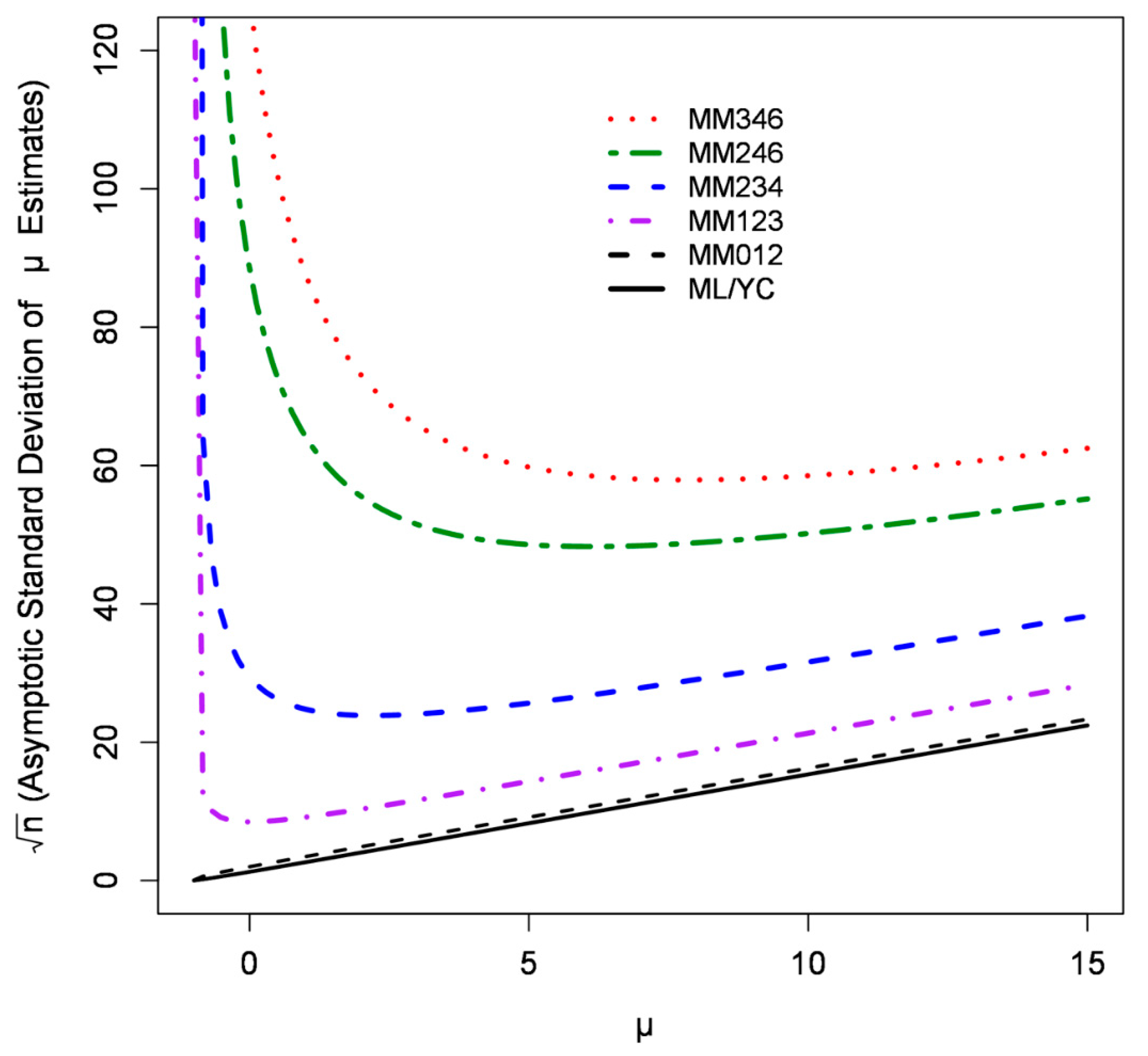
We started by examining the estimates of the shape parameter μ. The estimate standard deviations which follow from Table 2 (by taking square roots) are all of the form $1/\sqrt{n}$ multiplied by a function of (just) the shape parameter μ. In Figure 1, we take the ordinates to be $\sqrt{n}$ multiplied by the standard deviation to compare the large sample variabilities of all of the estimates listed in Table 1. To clarify, the curve displayed in Figure 1 associated the MM123 estimate of the shape parameter, for example, has ordinates $\sqrt{2(\mu +2)(\mu +3)(\mu +6)/(\mu +1)}.$

From Figure 1, we observe the moment estimates of the shape parameter incorporating the higher-order moments are least desirable as they have the highest variabilities, and the Ye/Chen and maximum likelihood estimates are most desirable as they have the lowest variabilities. The MM012 method has the smallest variability among the method of moments estimates and, in fact, compares favorably with the Ye/Chen and maximum likelihood methods.

The Ye/Chen and maximum likelihood curves are practically identical and appear as a single curve in Figure 1. Consequently, only the single key entry of “ML/YC” is given in the Figure 1 legend. No attempt is made here to analytically quantify how close these two standard deviation curves are, but this is largely a consequence of

$${\left[x\psi \prime (x)\right]}^2\cong 1+\psi \prime (x)$$

being a near identity over much of the region $x>-1.$

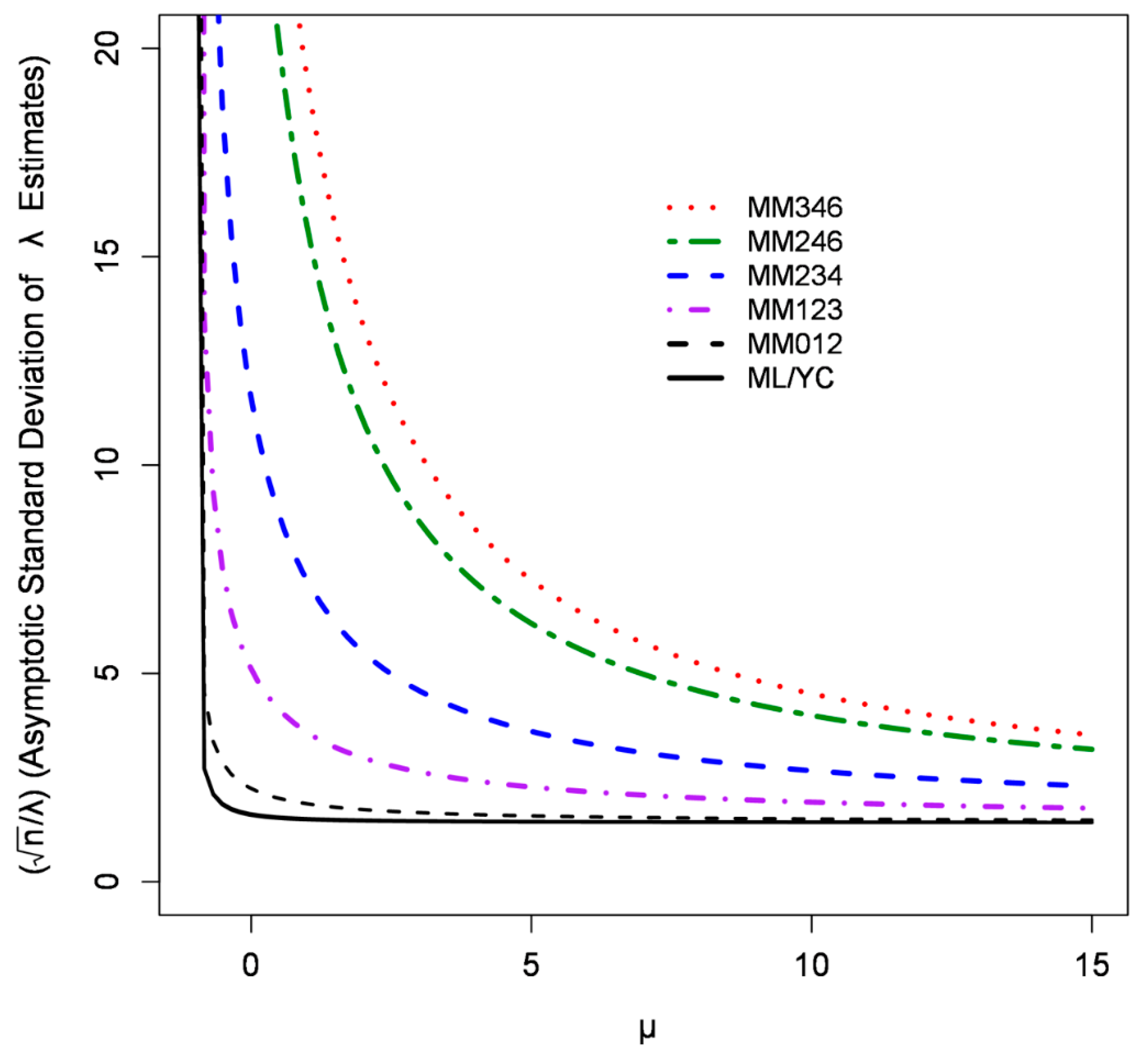
Now we turn to the estimates of the rate parameter λ. It will again be easiest to compare estimates graphically. All estimate standard deviations that follow from Table 2 (by taking square roots) are of the form $\lambda /\sqrt{n}$ multiplied by a function of (just) the shape parameter μ. In Figure 2, we take the ordinates to be $\sqrt{n}/\lambda$ multiplied by the standard deviation to compare the large sample variabilities of all of the estimates listed in Table 1. To clarify, the curve displayed in Figure 2 associated the MM123 estimate of the rate parameter, for example, has ordinates $\sqrt{(2{\mu }^2+23\mu +52)/(\mu +1)(\mu +2)}.$

As with the shape parameter, we see from Figure 2 that the moment estimates of the rate parameter incorporating the higher-order moments are least desirable as they have the largest variabilities, and the Ye/Chen and maximum likelihood estimates are the most desirable as they have the smallest variabilities. The MM012 method has the smallest variability among the method of moments estimates and compares favorably with the Ye/Chen and maximum likelihood methods.

The large sample variabilities given in Table 2 are attained, in a limiting sense, as the sample size grows. A natural question, then, is how large the sample size must be for these variabilities to hold to good approximation. A careful analysis would involve looking at both of the estimates $\widehat{\mu }$ and $\widehat{\lambda }$ across each of the seven different estimation procedures, with the behavior undoubtedly depending on the true parameter values of μ and λ. For our purposes here, we only very briefly discuss how empirical values of the standard deviations through simulated observations from a gamma RSD match-up to values from Table 2 for large samples in two cases: $\mu =2,\lambda =5$ and $\mu =5,\lambda =13$ (essentially the values used in [22]).

For a sample size of 2000 and both pairs of the shape and rate parameter values just stated, we found the relative errors in the standard deviations for the MM012, MM123, ML, and Ye/Chen $\widehat{\mu }$ and $\widehat{\lambda }$ estimates (but not the MM234, MM246, and MM346 estimates) to vary from about 1% to 3%. For the MM234 estimates with a sample size of 2000, we found relative errors for the standard deviations of the shape and rate parameters to each be about 1% in the case $\mu =5,\lambda =13$, but were each about 10% in the case $\mu =2,\lambda =5.$ Sample sizes larger than 2000 are needed for the variabilities listed for MM246 and MM346 in Table 2 to be reasonably accurate.

Increasing the sample size to 10,000, the MM246 and MM346 estimates had relative errors for the standard deviations of the shape and rate parameters to each be about 5% in the case $\mu =5,\lambda =13$ and to each be about 15% in the case $\mu =2,\lambda =5.$ Upon increasing the sample size to 100,000, these relative errors decreased to at most 0.8% in the case $\mu =5,\lambda =13$ and to 4% to 5% in the case $\mu =2,\lambda =5$ for both of these two method of moments procedures.

In practice, raindrop size samples are likely to be observed under stable conditions, corresponding to having fixed μ and λ parameter values, only over rather short time intervals, perhaps on the order of minutes. Multiple disdrometers would then be needed to collect sample sizes as large as, say 2000 drops. For more moderate sample sizes, the variabilities listed in Table 2 and displayed in Figure 1 and Figure 2 should not, of course, be fully trusted. However, the ranking of estimates according to variability given in Table 2 and Figure 1 and Figure 2 should persist to some degree as the sample size decreases and can be investigated through simulation. Such simulation for less than large sample sizes, however, is beyond the scope of this article.

4. Discussion and Conclusions

We used the delta method, a result known in the engineering and statistical literature, as a viable approach in deciding which of several gamma parameter estimates may be used when raindrop sizes can be accurately measured over the full spectrum of size. With the aid of the delta method, the estimates of the gamma shape and rate parameters listed in Table 1 were found, for large sample sizes, to be normal and unbiased with variances given in Table 2. Given several unbiased estimates, it is natural to prefer estimates with small variance.

If a method of moments procedure is to be used then to reduce estimate variance, we determined that gamma parameter estimates having the smallest order moments feasible should be preferred. We say ‘feasible’ as, for example, the lowest order moments might not always be reliable. Wind, for instance, can affect the reliability of the first moment. For some discussion related to this see, for example, [3,26,27].

We determined the maximum likelihood and pseudo maximum likelihood estimates of Table 1 have the smallest variances among the seven estimation procedures examined when estimating the gamma shape and rate parameters, but the MM012 method of moments procedure is very nearly as good in terms of variance.

When using instrumentation that does not accurately measure drop size over the full spectrum of drop size, then the variance results of Table 2 only hold approximately for large sample sizes. To compare gamma parameter estimates in this situation (or in the case of small sample size), samples of drop sizes from a gamma with known values of the shape and rate parameter may be randomly generated. Using these randomly generated samples, estimates may be compared in terms of their bias and variance. Such comparisons, for truncated and binned disdrometer data, were performed in [22] where we also suggested that the smallest order moments feasible be used when estimating gamma shape and rate parameters by method of moments.

References

1. Smith, J.A. Marked point process model of raindrop-size distributions. J. Appl. Meteorol. 1993, 32, 284–296. [Google Scholar] [CrossRef] [Green Version]
2. Ulbrich, C.W.; Atlas, D. Rainfall microphysics and radar properties: Analysis methods for drop size spectra. J. Appl. Meteorol. 1998, 37, 912–923. [Google Scholar] [CrossRef]
3. Vivekanandan, J.; Zhang, G.; Brandes, E. Polarimetric radar estimators based on a constrained gamma drop size distribution model. J. Appl. Meteorol. 2004, 43, 217–230. [Google Scholar] [CrossRef] [Green Version]
4. Ulbrich, C.W. Natural variation in the analytical form of the raindrop size distribution. J. Appl. Meteorol. Climatol. 1983, 22, 1764–1775. [Google Scholar] [CrossRef] [Green Version]
5. Kozu, T.; Nakamura, K. Rainfall parameter estimation from dual-radar measurements combining reflectivity profile and path-integrated attenuation. J. Atmos. Ocean. Technol. 1991, 8, 8–270. [Google Scholar] [CrossRef] [Green Version]
6. Tokay, A.; Short, D.A. Evidence from tropical raindrop spectra of the origin of rain from stratiform versus convective clouds. J. Appl. Meteorol. 1996, 35, 355–371. [Google Scholar] [CrossRef] [Green Version]
7. Brawn, D.; Upton, G. On the measurement of atmospheric gamma drop-size distributions. Atmos. Sci. Let. 2008, 9, 245–247. [Google Scholar]
8. Johnson, R.W.; Kliche, D.V.; Smith, P.L. Modeling raindrop size. J. Stat. Educ. 2015, 23. [Google Scholar] [CrossRef]
9. Smith, P.L. Raindrop size distributions: exponential or gamma–Does the difference matter? J. Appl. Meteorol. 2003, 42, 1031–1034. [Google Scholar] [CrossRef]
10. Rice, J. Mathematical Statistics and Data Analysis, 2nd ed.; Wadsworth, Inc.: Belmont, CA, USA, 1995; pp. 261–265. [Google Scholar]
11. Mallet, C.; Barthes, L. Estimation of gamma raindrop size distribution parameters: Statistical fluctuations and estimation errors. J. Atmos. Ocean. Technol. 2009, 26, 1572–1584. [Google Scholar] [CrossRef]
12. Kliche, D.V.; Smith, P.L.; Johnson, R.W. L-moment estimators as applied to gamma drop size distributions. J. Appl. Meteorol. Climatol. 2008, 47, 3117–3130. [Google Scholar] [CrossRef] [Green Version]
13. Johnson, R.W.; Kliche, D.V.; Smith, P.L. Comparison of estimators for parameters of gamma distributions with left-truncated samples. J. Appl. Meteorol. Climatol. 2011, 50, 296–310. [Google Scholar] [CrossRef]
14. Ye, Z.; Chen, N. Closed-form estimators for the gamma distribution derived from likelihood equations. Am. Stat. 2017, 71, 177–181. [Google Scholar]
15. Thurai, M.; Bringi, V.; Gatlin, P.N.; Petersen, W.A.; Wingo, M.T. Measurements and modeling of the full rain drop size distribution. Atmosphere 2019, 10, 39. [Google Scholar] [CrossRef] [Green Version]
16. Thurai, M.; Gatlin, P.; Bringi, V.N.; Petersen, W.; Kennedy, P.; Notaroš, B.; Carey, L. Toward completing the raindrop size spectrum: Case studies involving 2D-video disdrometer, droplet spectrometer, and polarimetric radar measurements. J. Appl. Meteorol. Climatol. 2017, 56, 877–896. [Google Scholar] [CrossRef]
17. Lawless, J.F. Statistical Models and Methods for Lifetime Data, 2nd ed.; John Wiley & Sons, Inc.: New York, NY, USA, 2003; pp. 539–540. [Google Scholar]
18. Doob, J.L. The limiting distributions of certain statistics. Ann. Math. Stat. 1935, 6, 160–169. [Google Scholar] [CrossRef]
19. Cramér, H. Mathematical Methods of Statistics; Princeton University Press: Princeton, NJ, USA, 1946. [Google Scholar]
20. Willis, P.T. Functional fits to some observed drop size distributions and parametrization of rain. J. Atmos. Sci. 1984, 41, 1648–1661. [Google Scholar] [CrossRef] [Green Version]
21. Chandrasekar, V.; Bringi, V.N. Simulation of radar reflectivity and surface measurements of rainfall. J. Atmos. Ocean. Technol. 1987, 4, 464–478. [Google Scholar] [CrossRef] [Green Version]
22. Johnson, R.W.; Kliche, D.V.; Smith, P.L. Maximum likelihood estimation of gamma parameters for coarsely binned and truncated raindrop size data. Q. J. R. Meteorol. Soc. 2014, 140, 1245–1256. [Google Scholar] [CrossRef]
23. Olver, F.W.J.; Lozier, D.W.; Boisvert, R.F.; Clark, C.W. (Eds.) NIST Handbook of Mathematical Functions; Cambridge University Press: Cambridge, UK, 2010; pp. 136–144. [Google Scholar]
24. Abramowitz, M.; Stegun, I.A. (Eds.) Handbook of Mathematical Functions; Dover Publications, Inc.: New York, NY, USA, 1972; p. 11. [Google Scholar]
25. Bowman, K.O.; Shenton, L.R. Properties of Estimators for the Gamma Distribution; Marcel Dekker, Inc.: New York, NY, USA, 1988; p. 30. [Google Scholar]
26. Rinehart, R.E. Out-of-level instruments: Errors in hydrometeor spectra and precipitation measurements. J. Appl. Meteorol. Climatol. 1983, 22, 1404–1410. [Google Scholar] [CrossRef] [Green Version]
27. Nešpor, V.; Krajewski, W.F.; Kruger, A. Wind-induced error of raindrop size distribution measurement using a two-dimensional video disdrometer. J. Atmos. Ocean. Technol. 2000, 17, 1483–1492. [Google Scholar] [CrossRef]
28. Brawn, D. Adapted GLM gamma parameter estimates for drop size distributions. Atmos. Sci. Let. 2015, 16, 386–390. [Google Scholar]
29. Miura, K. An introduction to maximum likelihood estimation and information geometry. Inter. Infor. Sci. 2011, 17, 155–174. [Google Scholar] [CrossRef] [Green Version]
30. Maplesoft, version 2018.2; Waterloo Maple Inc.: Waterloo, Canada, 2018.
Figure 1. Comparison of the large sample shape parameter estimate variabilities.
Atmosphere 11 00333 g001
Figure 2. Comparison of the large sample rate parameter estimate variabilities.
Atmosphere 11 00333 g002