Article

Improvement of Fog Simulation by the Nudging of Meteorological Tower Data in the WRF and PAFOG Coupled Model

Department of Atmospheric Sciences, Yonsei University, Seoul 03722, Korea
*
Author to whom correspondence should be addressed.
Atmosphere 2020, 11(3), 311; https://doi.org/10.3390/atmos11030311
Submission received: 28 January 2020 / Revised: 14 March 2020 / Accepted: 20 March 2020 / Published: 23 March 2020
(This article belongs to the Special Issue Observation, Simulation and Predictability of Fog )

Abstract

:
Improvement of fog simulation accuracy was investigated for the fogs that occurred on the south coast of the Korean Peninsula using the WRF (3D) and PAFOG (1D) coupled model. In total, 22 fog cases were simulated and accuracy of the fog simulation was examined based on Critical Success Index, Hit Rate and False Alarm Rate. The performance of the coupled WRF-PAFOG model was better than that of the single WRF model as expected. However, much more significant improvement appeared only when the data from a 300 m meteorological tower was not only used for the initial conditions but also nudged during the simulation. Moreover, a proper prescription of soil moisture was found to be important for accurate fog simulation especially for the fog cases with prior precipitation since efficient moisture supply from the precipitation-soaked soil might have been critical for fog formation. It was also demonstrated that with such optimal coupled model setting, a coastal radiation fog event with prior precipitation could be very realistically simulated: the fog onset and dissipation times matched so well with observation. In detail, radiative cooling at the surface was critical to form a surface inversion layer as the night fell. Then the vapor flux from the precipitation-soaked surface was confined within the inversion layer to form fog. It is suggested that a proper prescription of soil moisture in the model based on observations, if readily available, could be a cost-effective method for improving operational fog forecasting, considering the fact that tall meteorological towers are a rarity in the world.

1. Introduction

Fog has socioeconomic implications because significant decrease of visibility hinders aircraft operation, road traffic, shipping, air quality and crop productivity (e.g., Bartok et al., 2012; Klemm and Li, 2016 [1,2]). Indeed, restricted visibility due to fog can hamper safe navigation of ships, onshore marine traffic systems in coastal regions and can result in marine traffic accidents (e.g., Fu et al., 2010 [3]). Despite many previous studies to better understand fog formation mechanism better (e.g., Duynkerke 1991; Fuzzi et al., 1992; Wobrock et al., 1992; Nakanishi 2000; Gultepe et al., 2007; Fu et al., 2006; Shi et al., 2011; Pu et al., 2016; Lin et al., 2017 [4,5,6,7,8,9,10,11,12]), fog forecasting is challenging because the formation of fog is a consequence of complex and nonlinear interactions at various scales from the synoptic conditions to the micro scale and topographical conditions (Steeneveld and de Bode 2018 [13]).
Traditional fog prediction is based on statistical methods (e.g., Sujintjorn et al., 1994; Murtha, 1995; Marzban et al., 2007; Petty et al., 2000 [14,15,16,17]) or atmospheric models (e.g., Lin et al., 2017, Ballard et al., 1991, Koracin et al., 2005; van der Velde et al., 2010 [12,18,19,20]). A full three-dimensional (3D) numerical weather prediction (NWP) model is a promising technique because of its ability to simulate complex interactions for fog formation and dissipation. For example, Ballard et al. (1991) [18] attempted to use the numerical model of the United Kingdom Meteorological Office for fog forecasting. Koracin et al. (2005) [19] studied fog mechanism using 3D regional models and van der Velde et al. (2010) [20] attempted to forecast fog using Weather Research and Forecasting model (WRF) and High-Resolution Limited-Area Model (HIRLAM). Recently, Lin et al. (2017) [12] produced successful forecasting of an advection fog over the East China Sea using the WRF model. Despite such effort, even current 3D NWP models do not provide reliable fog prediction in a horizontal scales of <1 km especially over complex terrain and perfect initialization of soil moisture and temperature conditions for fog simulation cannot be achievable easily over a local terrain (Tang et al., 2009; Lim et al., 2012; Kim et al., 2019a [21,22,23]). On the other hand, one-dimensional (1D) model or linear model has been used for fog simulation because of its relatively small requirement of computing power (e.g., Bergot and Guedalia, 1994; Vosper, 2003 [24,25]). However, its application is limited because these simple models cannot handle horizontal heterogeneity properly.
It has been alternatively proposed to couple 1D models to 3D models to overcome the limitations of each approach for fog simulation. For example, Tang et al. (2009) [21] successfully simulated fog with NWP models with single forcing profiles from a radiosonde profile or from a low-resolution model. Shi et al. (2011) [10] developed a coupling method that inserted horizontal advection of heat and moisture from the simulation of a 3D regional model (MM5; NCAR mesoscale model) into a 1D turbulence model (PAFOG; PArameterized FOG model). Similarly, Kim and Yum (2012) [26] showed that a coupled system using the WRF and PAFOG model achieved better accuracy in fog simulation over the Yellow Sea. Similar coupled model approaches have also been applied to the studies of fogs at Paris Airport (Roquelaure and Bergot 2007; Bergot et al., 2005 [27,28]) and Casablanca airport (Bari 2019 [29]).
In this study, we investigated the accuracy of fog simulation over the southern coastal region of the Korean Peninsula. The main purpose of this study is to find the model setup that can best simulate the fog occurrence in this region. For this purpose, various different model setups (coupling, utilizing meteorological observation data as initial conditions, nudging of meteorological observation data, and utilizing observed soil moisture information) were examined and the impact of such different factors on the accuracy of fog simulation accuracy were analyzed. Then using the best model setup, we analysed the results of one fog case to assess the physical processes that were involved in this fog occurrence. Lastly, we assess the applicability of these results in operational fog forecasting.

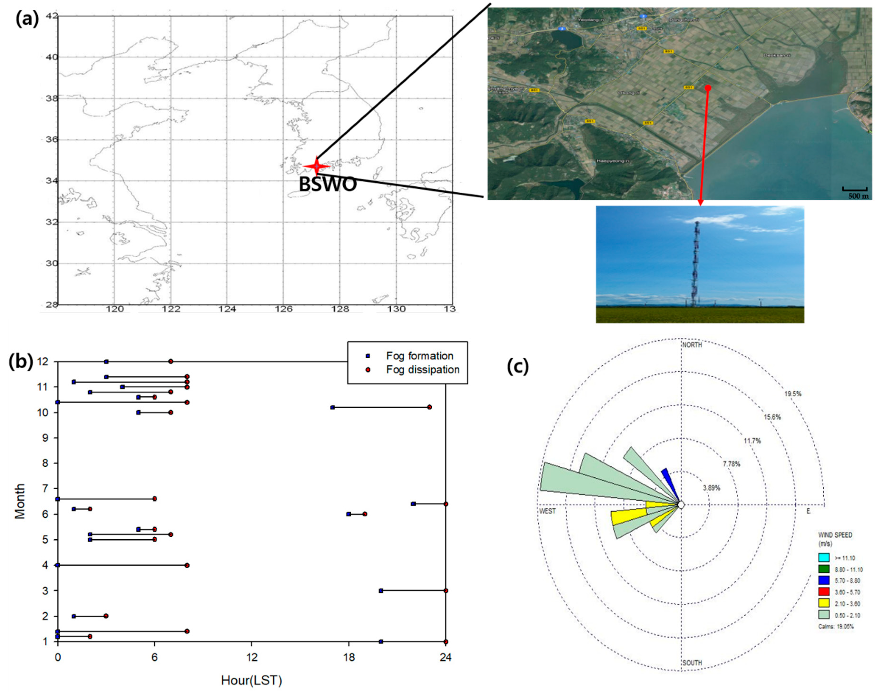
2. Observations and Methods

Boseong Standard Weather Observatory (BSWO) tower is 300 m high and located at the southern coast of the Korean Peninsula (34.7607° N, 127.2140° E) with a land cover of a double cropping rice paddy. Vertical profiles of air temperature (T), dew point temperature (Td), wind speed and wind direction have been measured at eleven different heights of the tower (i.e., 10 m, 20 m, 40 m, 60 m, 80 m, 100 m, 140 m, 180 m, 220 m, 260 m and 300 m). At the BSWO, comprehensive remote sensing measurements also have been done using a cloud radar, wind profiler, microwave radiometer and ceilometer. The T and Td at the surface were obtained from an AWS. The climate mean annual precipitation and air temperature at the BSWO was 1450 mm and 14 °C. More information on the BSWO can be found at Kim et al. (2019b) [30] and Hong et al. (2019) [31].
In our study, fog was identified if the observed visibility was less than 1 km and we investigated 22 fog cases observed at the BSWO for one year from May 2014 to June 2015 (Table 1). All 22 fog cases selected in this study were considered to be radiation fogs, since they formed during the night when radiative cooling was strong. Moreover, winds were from inland to the sea during the time of fog formation (Bari et al., 2015 [32]), barring moisture supply from the sea as a cause for fog formation (Figure 1).

3. Model and Numerical Experiments
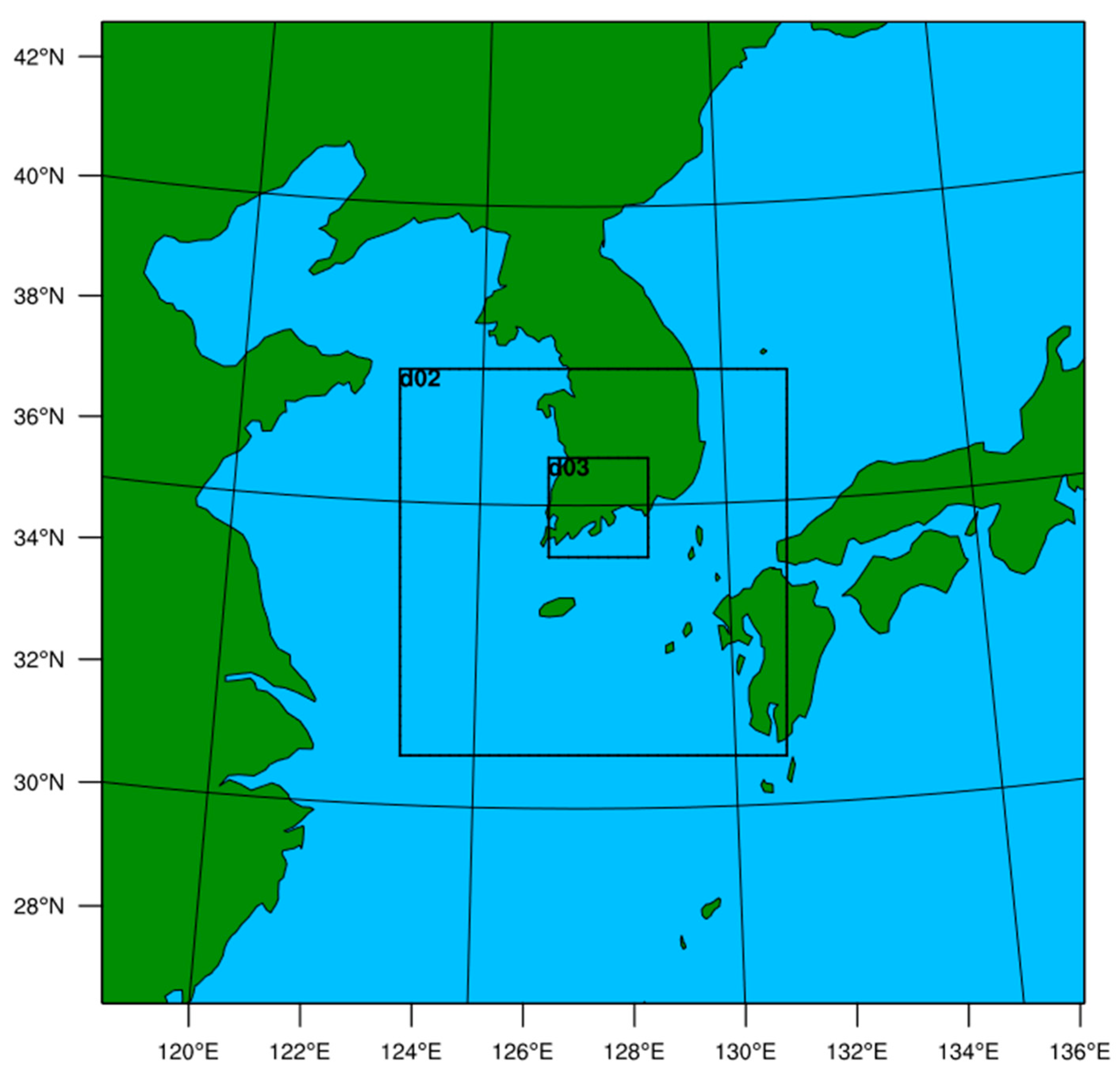
3.1. WRF Simulation

The WRF model ver. 3.7 (Skamarock et al., 2008) [33], was used as the 3D model to simulate fog formation and dissipation over the southern coastal area of the Korean Peninsula (Figure 2). One-way grid nesting procedure was used for the three domains. Domain 3, the finest horizontal resolution of 2 km, was centered at the BSWO and the model output from domain 3 was analyzed with the measurement data. The vertical layer consisted of 65 vertical layers. from the lowest eta level 0.998 (about 7 m above surface) to 50 hPa on a terrain-following hydrostatic-pressure vertical coordinate. The 6-hourly NCEP GDAS data were used as the initial and boundary conditions. The physics package included rapid radiation transfer scheme for general circulation models, the Mellor-Yamada-Nakanishi-Niino level 2.5 planetary boundary layer (PBL) scheme, Unified Noah land-surface model, Morrison 2-moments microphysics scheme (Table 2). We had tried various different model configurations and this configuration was found to the best configuration of the WRF model for the 22 fog cases selected in this study. The criteria for the selection of the best configuration was the same as those presented in this study. A brief description of all numerical simulations is given in Table 1.
The vertical layer consisted of 65 vertical layers. from the lowest eta level 0.998 (about 7 m above surface) to 50 hPa on a terrain-following hydrostatic-pressure vertical coordinate. The 6-hourly NCEP GDAS data were used as the initial and boundary conditions. The physics package included rapid radiation transfer scheme for general circulation models, the Mellor-Yamada-Nakanishi-Niino level 2.5 planetary boundary layer (PBL) scheme, Unified Noah land-surface model, Morrison 2-moments microphysics scheme (Table 2).

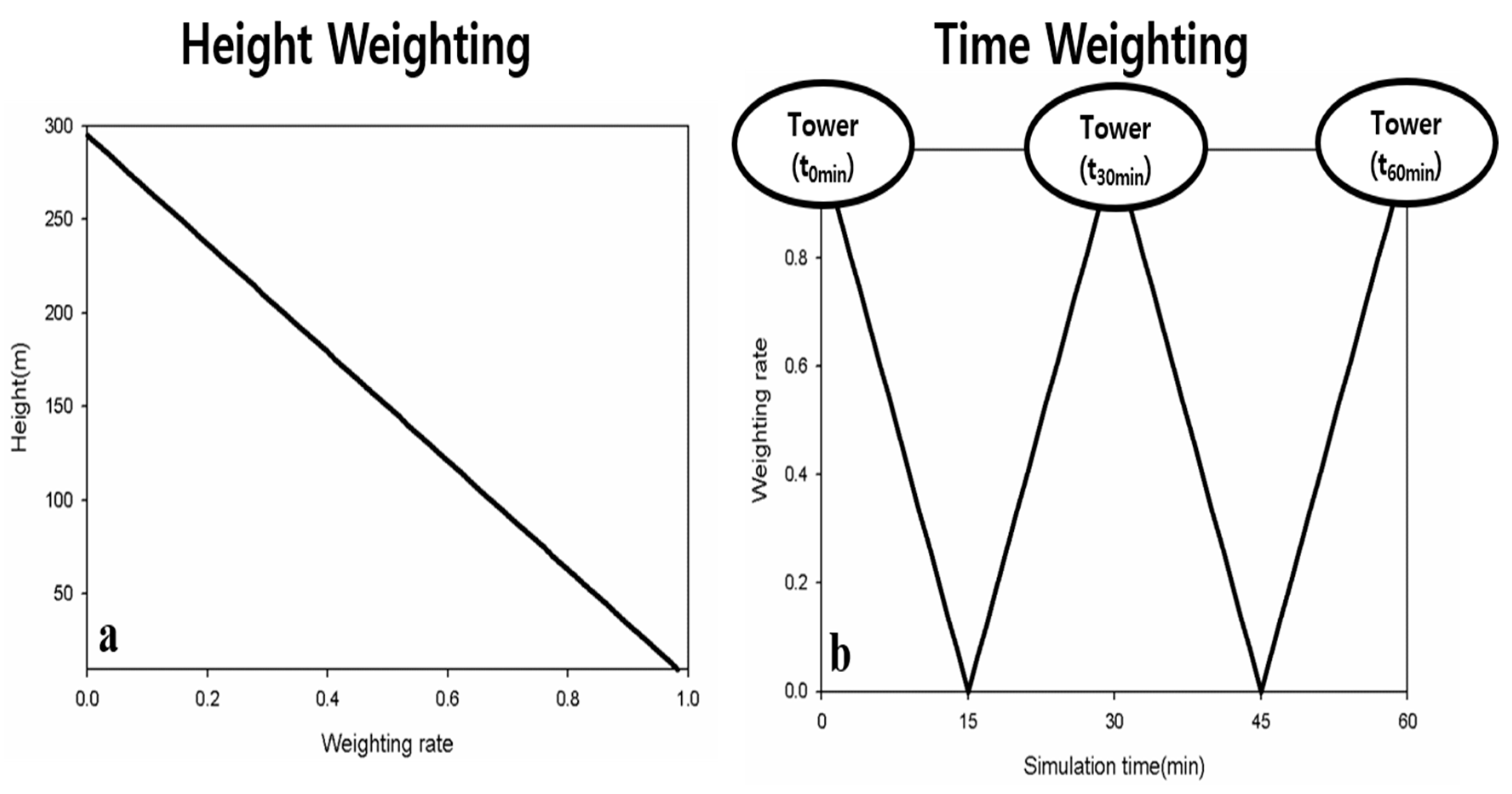
3.2. PAFOG Simulation

The PAFOG model is a 1D model of the atmospheric boundary layer consisting of the prognostic equations for horizontal wind field, potential temperature and specific humidity and was used to simulate fog formation observed at the BSWO on a meter scale. Previous studies reported that the PAFOG model reproduced temporal variation of important relevant parameters on the vertical column when suitable initial and boundary conditions were given (e.g., Bott and Trautmann, 2002; Kim and Yum, 2012 [26,34]). Solar radiation was calculated for the solar spectral interval of 0.28–6.00 μm and the infrared spectral interval of 3.5–100.0 μm, which includes the atmospheric window region of 8.75–12.25 μm (Zdunkowski et al., 1982 [35]). The microphysics scheme was based on double-moment parameterization (Nickerson et al., 1986; Chaumerlic et al., 1987 [36,37]) and the vegetation process was simulated following Siebert et al. (1992) [38]. The resolution of the model is 5 m from the surface to 1500 m and 10 m from 1500 m to the top of the model (i.e., 2500 m). More information on the PAFOG is available at Bott et al. (1990) [39], Bott and Trautmann (2002) [35] and Siebert et al. (1992) [38].
The 1D PAFOG model was coupled to the 3D WRF regional model (see Kim et al., 2019c [40] for details). Accordingly, boundary conditions for the PAFOG simulation were provided by the 3D WRF regional simulation. The initial conditions included geostrophic winds at 850 hPa, 2 m air temperature (Ta), surface pressure and the vertical profiles of pressure, air temperature and dew point temperature (Td). Moisture and heat advections in the PAFOG simulation were updated every hour to the governing equations of Ta and Td from the WRF model. Additional sensitivity experiments were performed, by using the observation data at the BSWO for initial and boundary conditions, and also by considering the impact of realistic boundary condition change by using the nudging technique (called Newtonian relaxation) (Figure 3). All the data observed at 10 different altitudes of the 300 m meteorological tower were nudged because it was found that using only the lower altitude data caused instability in model calculations. Moreover, during the nudging procedure, spatio-temporal weightings were applied for stable model integration without the discontinuity of model height and time (Figure 3). The weights increase toward the surface. This is reasonable because fog is mostly affected by the surface fluxes of moisture and heat and radiation budget at the surface and therefore the meteorological conditions at lower altitudes affect more on fog occurrence (Remy and Bergot, 2009 [41]). Details of all different numerical simulation settings are described in Table 3. For all fog cases, the model simulation started one day before the fog occurrence day and the total simulation time was 3 days (72 h). The first 24 h was considered to be a spin-up time for fog simulation.

3.3. Model Evaluation

To evaluate the performance of fog simulation, three statistical metrics were calculated: hit rate (HR), critical success index (CSI) and false alarm rate (FAR). HR is a measure of the model performance in simulating the observed fog and is estimated as:
HR = a a + c
FAR is a measure of the falsely simulating a fog and is estimated as:
FAR = b a + b
CSI is a measure of the fraction of forecast events that are correctly predicted and is estimated as:
CSI = a a + b + c
The symbols “a”, “b” and “c” indicate the correct hits, false hits and false rejections, respectively. The values of HR and CSI are unity and FAR is zero for a perfect model and there is a large difference between HR and CSI in case of a false fog alert when FAR is large (Wilks 2011 [42]). For the calculation of these indexes, existence or non-existence of fog was assessed hourly for the observation and model results. If fog existed at a particular one-hour interval in observation and the model also produced fog at that hour, it was considered to be a hit for that particular hour. Such hourly evaluation was made for an entire fog simulation time to calculate HR, FAR and CSI for that fog case.

4. Results and Discussion

4.1. Impact of the Observation Data on Fog Predictability

Previous studies reported that 3D atmospheric model itself did not reproduce the formation (onset) and dissipation times of fog mainly because of coarse horizontal and vertical resolutions (Boutle et al., 2015; Philip et al., 2016; Kim et al., 2019c [40,43,44]) or inappropriate turbulent cooling near the cold sea surface (Kim et al., 2019c [40]). Our 3D WRF simulations also did not capture the onset and dissipation times of fog events well as described in Table 4, where the performance statistics for various model settings are listed. Moreover, unlike some previous studies that had reported improvement of fog simulation in the coupled modeling system (e.g., Shi et al., 2011 (MM5 + PAFOG); Kim et al., 2019c (WRF + PAFOG) [10,40]), the coupled modeling system based on 1D PAFOG and 3D WRF models (WP) produced only slightly better HR (0.27 ± 0.30) and no substantial improvement of CSI (0.14 ± 0.18). The main cause of meager improvement was because fog dissipation time was not simulated well despite some improvement in fog onset time simulation. In addition, the large standard deviation of WP also indicates that HR values varied so much from case to case: HR ranged from 0.07 to 0.89.
There was dramatic increase of HR to 0.60 ± 0.48 when the observed meteorological data were used for the initial condition of the coupled model simulations (WPI). FAR rapidly increased in WPI experiments. Meanwhile, the improvement was even more impressive (HR = 0.81 ± 0.21) when these data were also nudged into the model (WPN). With decreases in FAR, CSI values also increased to 0.23 ± 0.18 and 0.45 ± 0.22 in the WPI and WPN simulations, respectively. Our findings suggest that it has substantial benefit to use the observation data in the coupled model for improving accuracy of fog simulation. These results are consistent with the results of previous studies that utilized observational data (e.g., Bergot et al., 2005; Roquelaure and Bergot 2007; Bari 2019 [27,28,29]). To note is that such improvement stemmed mostly from the simulations of radiation fog events (WPN_R).

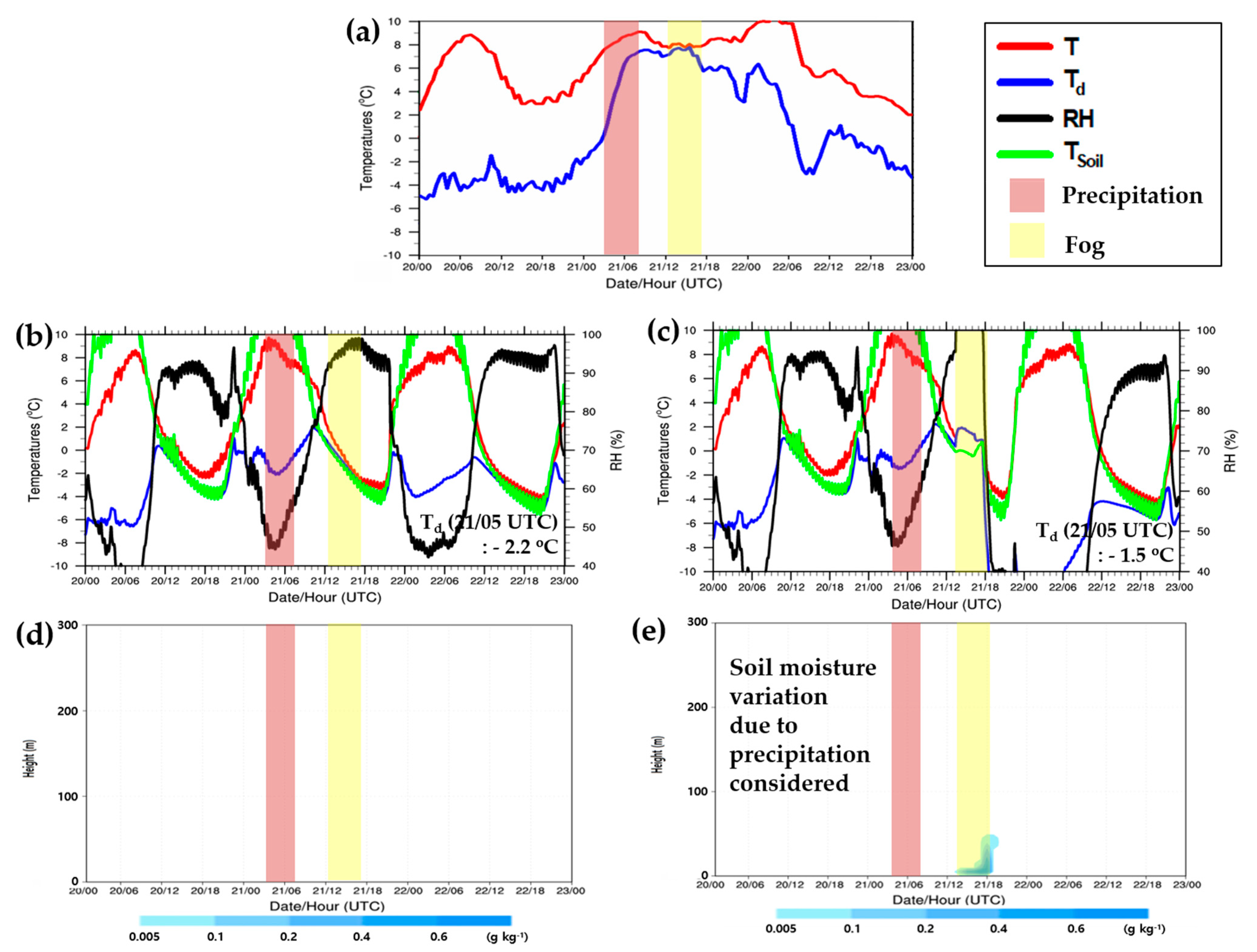
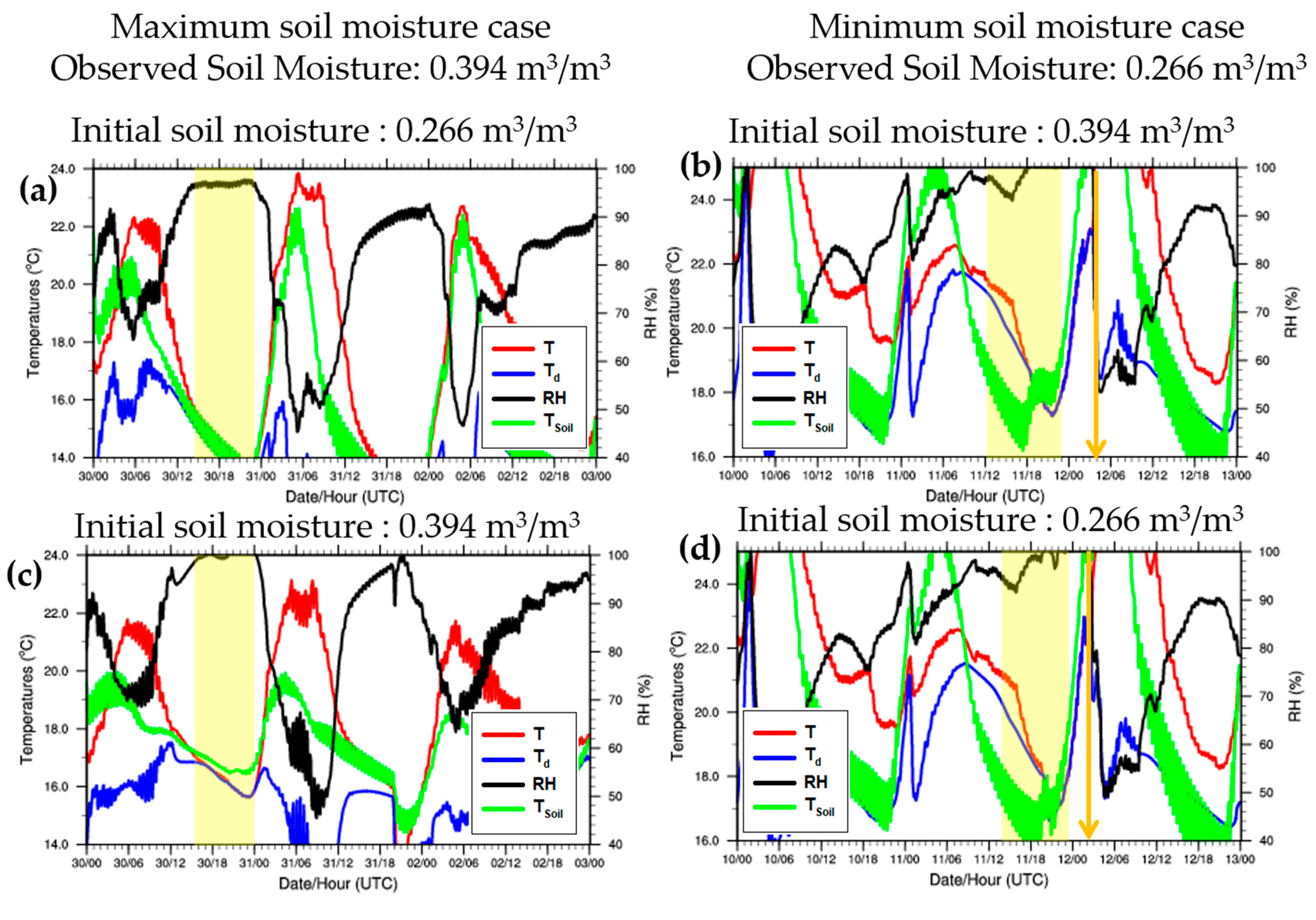
4.2. Impact of Precipitation and Soil Moisture

The coupled model with the nudging technique did not produce significantly better fog simulations for the cases in which precipitation occurred prior to the onset of fog (WPN_P), unlike its impressive improvement in radiation fog simulations (Table 4). Such unimpressive performance was suspected to be related to errors in soil moisture condition, which was directly related to precipitation. Since PAFOG is a fog model, precipitation cannot be simulated and the effect of precipitation on soil moisture content also cannot be considered. The impact of such precipitation bias on fog simulation were examined by analyzing the fog cases that had precipitation prior to the onset of fog. Figure 4 shows an example of such fog cases on 21 January 2015 (Case 11 in Table 1). Precipitation started at 04 UTC (13 LST) and lasted for 4 hours to 08 UTC (17 LST) with simultaneous increases of atmospheric humidity. The model did not capture the observed increase of Td during the precipitation because of precipitation bias and consequently fog formation was not simulated in the model (Figure 4b,d). In fact, the simulated soil moisture content value in the coupled model was lower than the value obtained from the 4D-Var data assimilation by the Korean Meteorological Administration (KMA) at the hours of precipitation. Notably, the sensitivity experiment with the replacement of soil moisture content to 0.316 m3 m−3 (from the KMA data assimilation system) for the time of precipitation showed better agreement with the observed fog formation (Figure 4c). With proper increase in soil moisture content, Td increased by about 0.7 °C (−2.2 °C to −1.7 °C) and the coupled model successfully captured the subsequent fog generation (Figure 4c,e).
Additional sensitivity experiments have been performed to illustrate the impact of reliable initial soil moisture information on fog simulation (Figure 5). For the two fog events where the observed soil moisture contents were the highest (Case 15 in Table 1, 0.394 m3 m−3) and the lowest (Case 22 in Table 1, 0.266 m3 m−3), we applied the opposite soil moisture content values and ran the coupled model simulations (Figure 5a,b). For Case 15, with the much smaller initial soil moisture content value than observation, the model failed to generate fog as evidenced by relative humidity (RH) lower than 100% (Figure 5a). For Case 22, with the much larger initial soil moisture content than observation, the model did not capture the fog dissipation time correctly, simulating longer than the observed duration of the fog event (Figure 5b). With the actual observed soil moisture content values as the initial condition, the model succeeded in generating fog (for Case 15, Figure 5c) and the fog dissipation time in the simulation almost exactly matched with the observation (for Case 22, Figure 5d). These results indicated that proper values of soil moisture content were critical for better fog simulation, along with nudging of the observation data.

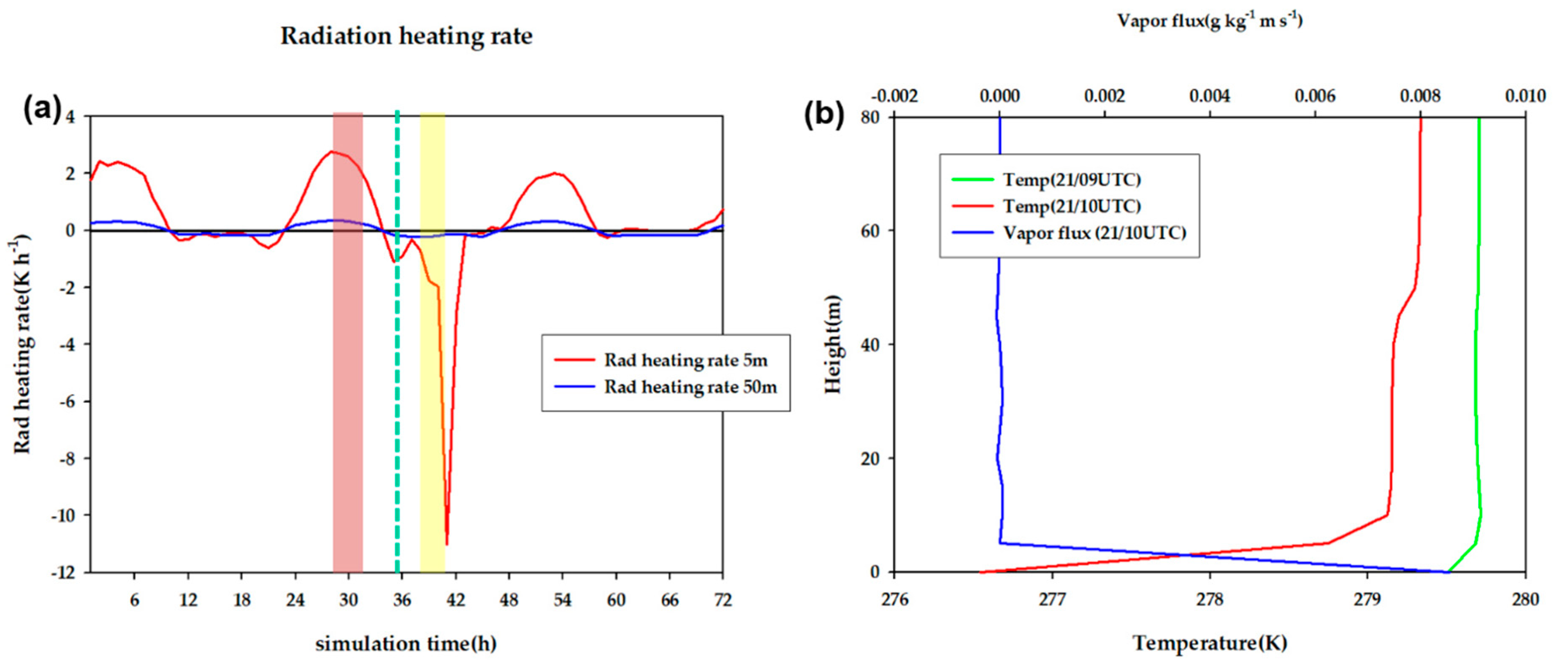
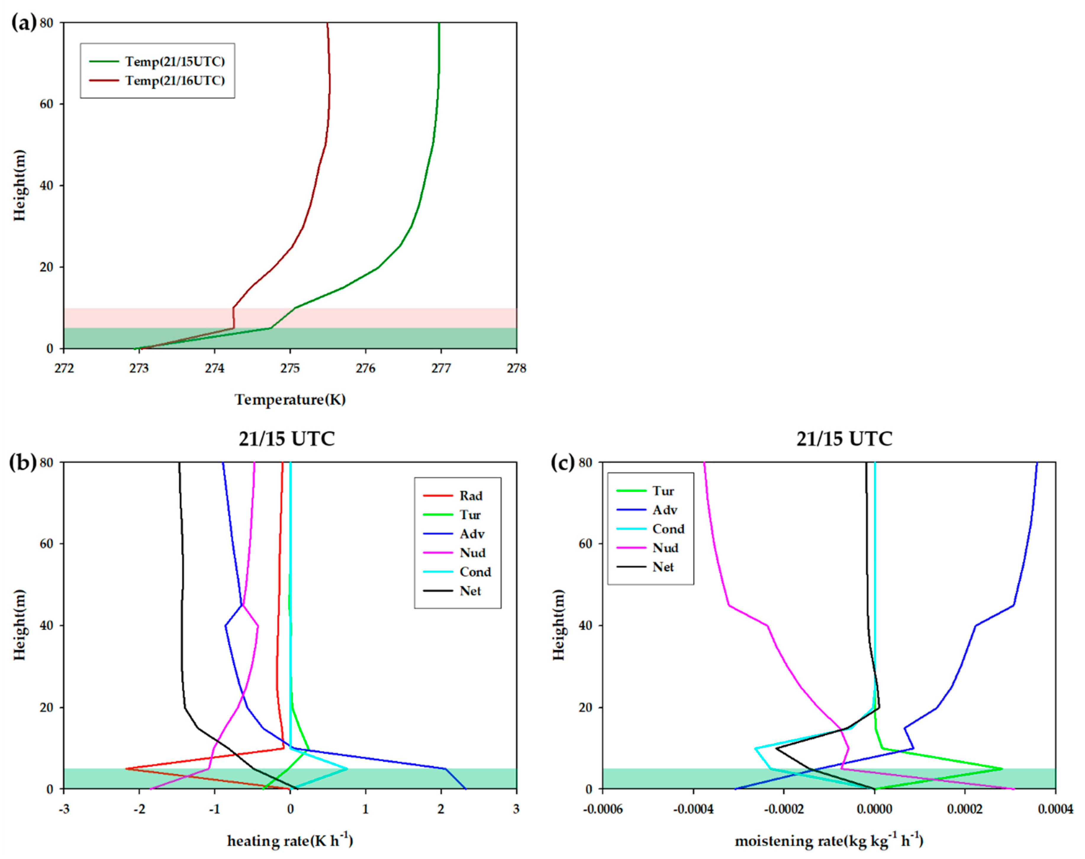
4.3. Case Study: Radiation Fog Generation Mechanism

Our study demonstrated that fog simulation could be improved by nudging the observation data and applying proper soil moisture content values. With such confidence, we highlighted a coastal radiation fog event with prior precipitation (Case 11 in Table 1) in more detail to understand better the controlling factors of such fog event in this region. As shown in Figure 4, the coupled model reproduced the observed fog formation and dissipation very well with observation data nudging and reliable soil moisture input. It rained for 4 h from 04 UTC (13 LST) and a strong inversion layer was developed around 10 UTC (19 LST). Figure 6a illustrates that as the night fell, radiative cooling rate (negative value of heating rate) near the surface (5 m altitude) became larger than that at 50 m altitude and at 10 UTC (green dashed vertical line) the difference became so significant to produce a surface inversion later as shown in Figure 6b. With weak turbulent mixing in the inversion layer, latent heat flux was nearly zero above the inversion layer and consequently water vapor evaporated from the surface was confined below the inversion layer (see the vapor flux profile in Figure 6b).
Such environment of radiative cooling and confined water vapor in the shallow inversion layer provided favorable conditions for fog formation several hours later (15 UTC) and the fog became thicker with time (Figure 7a). At 15 UTC, the heating rate was negative (meaning cooling) (Figure 7b) but the net moistening rate in the fog layer was negative (meaning drying) (Figure 7c). However, the main cause of drying was condensation in the fog and it was even more active above the fog top (see cyan line in Figure 7c), indicating that the fog top was rising. As the fog layer deepened, radiative cooling at the fog top and temperature increase in the fog layer largely due to condensational latent heating and warm advection weakened the inversion strength (see the temperature profiles up to the time of 17:30 UTC in Figure 8a).
Then all of a sudden the fog top rose as the temperature reduced abruptly in the fog layer (see 17:40 UTC in Figure 8a). However, moistening rate was not strong enough to maintain the whole fog layer and evaporation started to occur near the surface at 17:40 UTC (see that the net moistening rate was negative near the surface and the moistening rate due to condensation was positive in Figure 8c). With continued evaporation of fog drops and turbulent loss of moisture, fog started to dissipate near the surface to become a very shallow cloud, and then eventually dissipated completely (18:00 UTC). The evolution of the fog layer is clearly shown in Figure 4e.
Notable is that the nudging effect that seemed critical in the generation of the fog highlighted here. Earlier in the life cycle of the fog, the nudging effect was to cool the fog layer and also above the fog layer to reduce excessive heating (Figure 7b) and to remedy weak moistening in the fog layer and excessive moistening above the fog layer, which seemed to be caused mainly by excessive moisture advection (Figure 7c). However, the nudging effects were generally reduced in the later stage of the fog (Figure 8b,c), indicating that adjustment of the model results was not much necessary at this point. Without the nudging effects, fog might not have been generated for this fog case, although soil moisture adjustment due to prior precipitation was also critical as explained above.

5. Discussions and Conclusions

Fog simulation accuracy was investigated for the fogs occurred on the south coast of the Korean Peninsula using the WRF (3D) and PAFOG (1D) coupled model. For this purpose, we simulated 22 selected fog cases identified based on visibility measurements at BSWO, and the accuracy was examined based on CSI, HR and FAR. The low accuracy of fog simulation using the single WRF model was consistent with those demonstrated in previous studies (e.g., Boutle et al., 2015; Philip et al., 2016; Pu et al., 2016; Kim et al., 2019a; Kim et al., 2019c [11,23,40,43,44]). Improvement in the performance of the WRF and PAFOG coupled model over the single WRF model was also consistent with previous studies (e.g., Kim and Yum, 2012, 2013 [26,45]). However, such improvement of the coupled model was not very impressive. When the data from a 300 m meteorological tower at BSWO was not only used for the initial conditions but also nudged during the simulation, the accuracy of the coupled model for fog simulation was significantly improved. Further improvement was achieved when observed soil moisture content information was utilized as initial condition, instead of using the values prescribed by the soil type of BSWO as initial condition. Nevertheless, such improvement was not visible for the fog cases with prior precipitation, apparently because the model could not consider the soil moisture change caused by precipitation. When the soil moisture condition for the time of precipitation was adjusted to the values obtained from data assimilation for that time, accuracy of fog simulation became much better.
With confidence on the coupled model performance, we examined a coastal radiation fog event with prior precipitation in more detail to understand better the controlling factors of such fog event in this region. Radiative cooling at the surface was critical to form a surface inversion layer as the night fell. Then the vapor flux from the surface was confined within the inversion layer to form fog. With fog top radiative cooling, inversion strength weakened but with continued vapor flux from the surface, eventually the fog top rose abruptly. However, moisture supply from the surface became not strong enough to maintain the whole fog layer and the fog started to dissipate near the surface to become a shallow cloud before it dissipated completely. Such evolution of the fog layer (i.e., onset and dissipation times) in the model simulation were well matched by the observation (Figure 4e).
Numerical fog simulation has been known to be notoriously difficult, but we demonstrated in this study that very realistic fog simulation was possible with concerted effort to utilize available observational data that are relevant to fog such as temperature and humidity profiles and soil moisture. We insist that the coupled model system with nudging introduced in this study can be used for more detailed study of fog formation and dissipation mechanisms. Perhaps a tall meteorological tower data may not be available in most places despite the critical improvement of fog simulation by nudging the tower data. One of the main purposes of doing fog simulation studies is to apply what we learn from such studies to the improvement of operational fog forecasting. However, nudging technique itself is not applicable when it comes to operational fog forecasting. In that sense, a proper prescription of soil moisture in the model based on observations, if readily available, could be a cost-effective method for improving operational fog forecasting. The improvement of WPS is significant when compared to WRF or WP in Table 4. The numerical simulation setting of WPS would be practically applicable to operational fog forecasting and therefore is recommended for operational fog forecasting.

Author Contributions

Formal analysis, J.I.S.; writing—original draft, W.K.; writing—review and editing, S.S.Y. and J.H. All authors have read and agreed to the published version of the manuscript.

Funding

This work was supported by the National Research Foundation of Korea (NRF) grant funded by the Korea government (MSIT) (No. NRF-2018R1A2B2006965).

Acknowledgments

The use of PAFOG was developed by the University of Bonn in Germeny.

Conflicts of Interest

The authors declare no conflicts of interest.

References

  1. Bartok, J.; Bott, A.; Gera, M. Fog prediction for road traffic safety in a coastal desert region. Bound. Layer Meteorol. 2012, 145, 485–506. [Google Scholar] [CrossRef]
  2. Klemm, O.; Lin, N. What causes observed fog trends: Air quality or climate change. Aerosol Air Qual. Res. 2016, 16, 1131–1142. [Google Scholar] [CrossRef]
  3. Fu, G.; Li, P.; Crompton, J.G.; Guo, J.; Gao, S.; Zhang, S. An observational and modeling study of a sea fog event over the Yellow Sea on 1 August 2003. Meteorol. Atmos. Phys. 2010, 107, 149–159. [Google Scholar] [CrossRef]
  4. Duynkerke, P.G. Radiation Fog: A comparison of model simulation with detailed observations. Mon. Wea. Rev. 1991, 119, 324–341. [Google Scholar] [CrossRef] [Green Version]
  5. Fuzzi, S.; Facchini, M.C. The Po valley fog experiment 1989. Tellus 1992, 44, 448–468. [Google Scholar] [CrossRef] [Green Version]
  6. Wobrock, W.; Facchini, M.C. Meteorological characteristics of the Po valley fog. Tellus 1992, 44, 469–488. [Google Scholar] [CrossRef]
  7. Nakanishi, J. Large-eddy simulation of radiation fog. Bound. Layer Meteorol. 2000, 94, 461–493. [Google Scholar] [CrossRef]
  8. Gultepe, I.; Tardif, R.; Michaelides, S.C.; Cermak, J.; Bott, A.; Bendix, J.; Muller, M.D.; Pagowski, M.; Hansen, B.; Ellrod, G.W.; et al. Fog Research: A Review of Past Achievements and Future Perspectives. Pure Appl. Geophys. 2007, 164, 1420–9136. [Google Scholar] [CrossRef]
  9. Fu, G.; Guo, J.T.; Xie, S.P.; Duane, Y.H.; Zhang, M.G. Analysis and high-resolution modeling of a dense sea fog event over the Yellow Sea. Atmos. Res. 2006, 81, 293–303. [Google Scholar] [CrossRef]
  10. Shi, C.; Wang, L.; Zhang, H.; Zhang, S.; Deng, X.; Li, Y.; Qiu, M. Fog simulations based on multi-model system:a feasibility study. Pure Appl. Geophys. 2011. [Google Scholar] [CrossRef]
  11. Pu, Z.; Chachere, C.; Hoch, S.; Pardyjak, E.; Gultepe, I. Numerical prediction of cold season fog events over complex terrain: The performance of the WRF model during MATERHORN-Fog and early evaluation. Pure Appl. Geophys. 2016, 173, 3165–3186. [Google Scholar] [CrossRef]
  12. Lin, C.Y.; Zhang, Z.F.; Pu, Z.X.; Wang, F. Numerical simulations of an advection fog event over Shanghai Pudong International Airport with the WRF model. J. Meteorol. Res. 2017, 31, 874–889. [Google Scholar] [CrossRef]
  13. Steeneveld, G.Y.; De Bode, M. Unravelling the relative roles of physical processes in modelling the life cycle of a warm radiation fog. Q. J. R. Meteorol. Soc. 2018, 144, 1539–1554. [Google Scholar] [CrossRef]
  14. Sujitjorn, S.; Sookjaras, P.; Wainikorn, W. An expert system to forecast visibility in Don-Muang Air Force Base. In 1994 IEEE International Conference on Humans, Information and Technology, Systems Man and Cybernetics; IEEE: Piscataway, NJ, USA, 1994; Volume 3, pp. 2528–2531. [Google Scholar]
  15. Murtha, J. Applications of fuzzy logic in operational meteorology. Can. Forces Weather Serv. 1995, 42–54. [Google Scholar]
  16. Marzban, C.; Leyton, S.M.; Colman, B. Ceiling and visibility forecasts via neural networks. Weather Forecast. 2007, 22, 466–479. [Google Scholar] [CrossRef] [Green Version]
  17. Petty, K.; Carmichael, B.; Wiener, G.; Petty, M.; Limber, M. A fuzzy logic system for the analysis and prediction of cloud ceiling and visibility. Preprints Ninth Conference on Aviation, Range, and Aerospace Meteorology, Orlando, F1. Am. Meteor. Soc. 2000, 331–333. [Google Scholar]
  18. Ballard, S.P.; Golding, B.W.; Smith, R.N.B. Mesoscale model experimental forecasts of the haar of northeast Scotland. Mon. Weather Rev. 1991, 119, 2107–2123. [Google Scholar] [CrossRef] [Green Version]
  19. Koracin, D.; Businger, J.; Dorman, C.; Lewis, J. Formation, evolution, and dissipation of coastal sea fog. Bound. Layer Meteorol. 2005, 117, 447–478. [Google Scholar] [CrossRef]
  20. Van der Velde, I.R.; Steeneveld, G.J.; Wichers Schreur, B.G.J.; Holtslag, A.A.M. Modeling and forecasting the onset and duration of severe radiation fog under frost conditions. Mon. Weather Rev. 2010, 138, 4237–4253. [Google Scholar] [CrossRef]
  21. Tang, Y.M.; Capon, R.; Forbes, R.; Clark, P. Fog prediction using a very high resolution numerical weather prediction model forced with a single profile. Meteorol. Appl. 2009, 16, 129–141. [Google Scholar] [CrossRef]
  22. Lim, Y.; Hong, J.; Lee, J.T.-Y. Spin-up behavior of soil moisture in a land surface model for East Asia. Meteorol. Atmos. Phys. 2012, 118, 151–161. [Google Scholar] [CrossRef]
  23. Kim, C.K.; Yum, S.S.; Kim, H.Y.; Kang, Y.H. A WRF modeling study on the effects of land use changes on fog off the west coast of the korea peninsula. Pure Appl. Geophys. 2019. [Google Scholar] [CrossRef]
  24. Bergot, T.; Guedalia, D. Numerical forecasting of radiation fog. Part I: Numerical model and sensitivity tests. Mon. Weather Rev. 1994, 122, 1218–1230. [Google Scholar] [CrossRef] [Green Version]
  25. Vosper, S. Development and testing of a high resolution mountainwave forecasting system. Meteorol. Appl. 2003, 10, 75–86. [Google Scholar] [CrossRef] [Green Version]
  26. Kim, C.K.; Yum, S.S. A numerical study of sea fog formation over cold sea surface using a one-dimensional turbulence model coupled with the Weather Research and Forecasting Model. Bound. Layer Meteorol. 2012, 143, 481–505. [Google Scholar] [CrossRef]
  27. Bergot, T.; Carrer, D.; Noilhan, J.; Bougeault, P. Improved site-specific numerical prediction of fog and low clouds: A feasibility study. Weather Forecast. 2005, 20, 627–646. [Google Scholar] [CrossRef] [Green Version]
  28. Roquelaure, S.; Bergot, T. Seasonal sensitivity on COBEL-ISBA local forecast system for fog and low clouds. Pure Appl. Geophys. 2007, 164, 1283–1301. [Google Scholar] [CrossRef]
  29. Bari, D. A Preliminary Impact Study of Wind on Assimilation and Forecast Systems into the One-Dimensional Fog Forecasting Model COBEL-ISBA over Morocco. Atmosphere 2019, 10, 615. [Google Scholar] [CrossRef] [Green Version]
  30. Kim, H.; Hong, J.-W.; Lim, Y.; Hong, J.; Shin, S.; Kim, Y. Evaluation of JULES land surface model based on in-situ data of NIMS flux sites. Atmosphere 2019, 29, 355–365. (In Korean) [Google Scholar]
  31. Hong, J.-W.; Hong, J.; Chun, J.; Lee, Y.; Chang, L.; Lee, J.; Yi, K.; Park, Y.; Byun, Y.; Joo, S. Comparative assessment of net CO2 exchange across an urbanization gradient in Korea based on in situ observation. Carbon Balance Manag. 2019. [Google Scholar] [CrossRef] [Green Version]
  32. Bari, D.; Bergot, T.; Khlifi, M.E. Local meteorological and large scale weather characteristics of fog over the Grand Casablanca region, Morocco. J. Appl. Meteorol. Climatol. 2016, 55, 1731–1745. [Google Scholar] [CrossRef]
  33. Skamarock, W.C.; Klemp, J.B.; Dudhia, J.; Gill, D.O.; Barker, D.M.; Duda, M.G.; Huang, X.-Y.; Wang, W.; Powers, J.G. A Description of the Advanced Research WRF Version 3. NCAR Technical Note NCAR/TN-475+STR; National Center for Atmospheric Research: Boulder, CO, USA, 2008; 125p. [Google Scholar]
  34. Bott, A.; Trautmann, T. PAFOG-a new efficient forecast model of radiation fog and low-level stratiform clouds. Atmos. Res. 2002, 64, 191–203. [Google Scholar] [CrossRef]
  35. Zdunkowski, W.G.; Panhans, W.-G.; Welch, R.M.; Korb, J.G. A radiation scheme for circulation and climate models. Beitr. Phys. Atmos. 1982, 55, 215–238. [Google Scholar]
  36. Nickerson, E.C.; Richard, E.; Rosset, R.; Smith, R.D. The numerical simulation of clouds, rain, and airflow over the Vosges and Black Forest mountains: A meso-h model with parameterized microphysics. Mon. Weather Rev. 1986, 114, 398–414. [Google Scholar] [CrossRef] [Green Version]
  37. Chaumerliac, N.; Richard, E.; Pinty, J.P.; Nickerson, E.C. Sulfur scavenging in a mesoscale model with quasi-spectral microphysics: Two-dimensional results for continental and maritime clouds. J. Geophys. Res. 1987, 92, 3114–3126. [Google Scholar] [CrossRef]
  38. Siebert, J.; Sievers, U.; Zdunkowski, W. A one-dimensional simulation of the interaction between land surface processes and the atmosphere. Bound. Layer Meteorol. 1992, 59, 1–34. [Google Scholar] [CrossRef]
  39. Bott, A.; Sievers, U.; Zdunkowski, W. A radiation fog model with a detailed treatment of the interaction between radiative transfer and fog microphysics. J. Atmos. Sci. 1990, 47, 2153–2166. [Google Scholar] [CrossRef] [Green Version]
  40. Kim, W.; Kim, C.K.; Yum, S.S. Numerical Simulation of Sea Fog over the Yellow Sea: Comparison between UM+ PAFOG and WRF+ PAFOG Coupled Systems. Asia-Pac. J. Atmos. Sci. 2019. [Google Scholar] [CrossRef]
  41. Rémy, S.; Bergot, T. Assessing the impact of observations on a local numerical fog prediction system. Q. J. R. Meteorol. Soc. 2009, 135, 1248–1265. [Google Scholar]
  42. Wilks, D.S. Statistical Methods in the Atmospheric Sciences, 3rd ed.; Academic Press: Cambridge, UK, 2011. [Google Scholar]
  43. Boutle, I.; Finnenkoetter, A.; Lock, A.; Wells, H. The London model: Forecasting fog at 333 m resolution. Q. J. R. Meteorol. Soc. 2015. [Google Scholar] [CrossRef]
  44. Philip, A.; Bergot, T.; Bouteloup, Y.; Bouyssel, F. The impact of vertical resolution on fog forecasting in the kilometric-scale model AROME: A case study and statistics. Weather Forecast. 2016, 31, 1655–1671. [Google Scholar] [CrossRef]
  45. Kim, C.K.; Yum, S.S. A study on the transition mechanism of stratus cloud in fog over warm sea surface using a single column model coupled with WRF, Asia-Pac. J. Atmos. Sci. 2013, 49, 245–257. [Google Scholar]
Figure 1. (a) Location of Boseong Standard Weather Observatory (BSWO); (b) fog onset and dissipation time for each fog case; and (c) wind rose distribution during the fogs.
Atmosphere 11 00311 g001
Figure 2. Domain setting of the 3D Weather Research and Forecasting (WRF) model.
Atmosphere 11 00311 g002
Figure 3. Weighting rates of height and time for the nudging. (a) Height Weighting; (b) Time Weighting.
Atmosphere 11 00311 g003
Figure 4. (a) Time variation of T and Td measured at BSWO for the highlighted fog case (January 21, 2015; Case 11 in Table 1); (b) time variations of T, Td, RH and Ts, and (d) liquid water mixing ratio from the coupled model simulation with no consideration of the precipitation effect on soil moisture; and (c), (e) with such consideration. The observed fog (21/14 UTC–21/18 UTC) and precipitation (21/04 UTC–21/08 UTC) times are shaded yellow and brown, respectively. The simulation started at 00 UTC January 20 and lasted 72 h.
Atmosphere 11 00311 g004
Figure 5. Time variations of T, Td, RH and Ts from the simulations for the maximum and minimum soil moisture cases (a), (b) when the opposite soil moisture content values were applied and (c), (d) when the actual soil moisture content values were applied. The observed time of fog is shaded yellow. The orange arrow in (b) and (d) indicates fog dissipation time in each simulation.
Atmosphere 11 00311 g005
Figure 6. (a) Time variation of radiative heating rates at 5 m and 50 m and (b) vertical profiles of temperature and vapor flux at relevant times for the fog case depicted in Figure 4. Precipitation period is marked with red vertical bar and observed fog period is shaded yellow. The vertical dash green line refers to 10 UTC.
Atmosphere 11 00311 g006
Figure 7. (a) Vertical profiles of temperature at earlier times (15 UTC and 16 UTC) of fog development in the coupled model simulation of the fog case depicted in Figure 4; and vertical profiles of various components of (b) heating rates and (c) moistening rates. The shading indicates the fog layer at 15 UTC (green) and 16 UTC (brown).
Atmosphere 11 00311 g007
Figure 8. Same as Figure 7 except (a) the vertical profiles of temperature at later times and vertical profile of (b) heating rates and (c) moistening rates at 17:40 UTC. The blue shading indicates the fog layer.
Atmosphere 11 00311 g008
Table 1. List of 22 fog cases.
No.DateFog TypeNo.DateFog Type
109-10-2014Radiation fog case1201-26-2015Case with prior precipitation
214-10-2014Radiation fog case1302-22-2015Case with prior precipitation
310-20-2014Case with prior precipitation1403-30-2015Radiation fog case
410-25-2014Radiation fog case1503-31-2015Case with prior precipitation
510-26-2014Radiation fog case1605-01-2015Radiation fog case
611-05-2014Radiation fog case1705-02-2015Radiation fog case
711-22-2014Radiation fog case1805-19-2015Radiation fog case
811-27-2014Radiation fog case1906-03-2015Case with prior precipitation
912-08-2014Case with prior precipitation2006-09-2015Radiation fog case
1012-20-2014Case with prior precipitation2106-10-2015Radiation fog case
1101-21-2015Case with prior precipitation2206-11-2015Case with prior precipitation
Table 2. Summary of the 3D model setting.
CategoryWRF V3.7
Horizontal Resolution18, 6, 2 km
Vertical Layers65 (top~20 km)
20 (below 1 km)
Initial fieldNCEP (National Center for Environmental Prediction) GDAS (Global Data Assimilation System) data
Radiation ProcessRRTMg (Rapid Radiative Transfer model) scheme (both SW & LW)
PBL ProcessMYNN(Mellor-Yamada Nakanish Niino) scheme
Surface physicsUnified Noah land-surface model
MicrophysicsMorrison
Table 3. Description of different numerical simulation settings.
AbbreviationNumber of SimulationsDescription
WRF22Single WRF simulations with the experimental design in Table 1
WP22The coupled model (WRF + PAFOG) simulation
WPI22Same as WP except that the tower observed meteorological data is utilized for initial conditions
WPN22Same as WP except that the tower observed meteorological data are utilized as initial conditions and periodically nudged into the coupled model
WPS22Same as WPI except that observed soil moisture content information is utilized as initial condition
WPNS22Same as WPN except that observed soil moisture content information is also utilized as initial condition
WPN_R13WPN but only for the radiation fog events
WPN_P9WPN but only for the fog events with prior precipitation
WPNS_P9WPNS except that during the time of prior precipitation soil moisture content value is replaced by the value from KMA data assimilation
Table 4. Model performance statistics for different numerical simulation settings. Shown are average and standard deviation of hit rate (HR), critical success index (CSI) and false alarm rate (FAR).
Numerical Simulation SettingHRCSIFAR
WRF0.15 ± 0.120.11 ± 0.230.05 ± 0.04
WP0.27 ± 0.300.14 ± 0.180.21 ± 0.22
WPI0.60 ± 0.480.23 ± 0.180.49 ± 0.41
WPN0.81 ± 0.210.45 ± 0.220.39 ± 0.22
WPS0.53 ± 0.350.27 ± 0.190.33 ± 0.28
WPNS0.89 ± 0.070.64 ± 0.130.25 ± 0.10
WPN_R0.93 ± 0.160.65 ± 0.240.28 ± 0.25
WPN_P0.68 ± 0.240.26 ± 0.130.52 ± 0.18
WPNS_P0.82 ± 0.480.50 ± 0.080.34 ± 0.44

