Improving Ensemble Forecasting Using Total Least Squares and Lead-Time Dependent Bias Correction

Abstract

Numerical weather prediction (NWP) models produce a quantitative precipitation forecast (QPF), which is vital for a wide range of applications, especially for accurate flash flood forecasting. The under- and over-estimation of forecast uncertainty pose operational risks and often encourage overly conservative decisions to be made. Since NWP models are subject to many uncertainties, the QPFs need to be post-processed. The NWP biases should be corrected prior to their use as a reliable data source in hydrological models. In recent years, several post-processing techniques have been proposed. However, there is a lack of research on post-processing the real-time forecast of NWP models considering bias lead-time dependency for short- to medium-range forecasts. The main objective of this study is to use the total least squares (TLS) method and the lead-time dependent bias correction method—known as dynamic weighting (DW)—to post-process forecast real-time data. The findings show improved bias scores, a decrease in the normalized error and an improvement in the scatter index (SI). A comparison between the real-time precipitation and flood forecast relative bias error shows that applying the TLS and DW methods reduced the biases of real-time forecast precipitation. The results for real-time flood forecasts for the events of 2002, 2007 and 2011 show error reductions and accuracy improvements of 78.58%, 81.26% and 62.33%, respectively.

1. Introduction

It is essential that quantitative precipitation forecasts (QPFs) provide precise estimation and forecasts for a wide range of applications, including hydrology, meteorology, agriculture, hydrometeorology, and other related areas of study. The QPFs produced by numerical weather prediction (NWP) models are vital for water resource management, especially for accurate flash flood forecasting [1], because they are the main input to hydrological models for flood forecasting [2]. The reliability and practical use of flood forecasting is directly connected to the accuracy of QPFs. Skillful QPFs provide better information on extreme floods [3]. Underestimation of the forecast data causes operational risks, while overestimation induces overly conservative solutions. Attaining correct and reliable flood forecasts using high-quality QPFs has a significant effect on early flood warnings and the scheduling of evacuations, allowing water managers to make robust decisions [2].

NWP models are highly nonlinear and uncertainties related to the model outputs are still poorly understood [4]. The capability of the NWP model forecasting system to produce forecasts is related to different factors, such as physical parameterization schemes, initial and boundary conditions, and horizontal and vertical resolution [5,6,7]. The complexity involved in forecasting is extensive, and precipitation has the most complex behavior compared to other meteorological forecasts. Errors in NWP model forecasts are caused by incomplete and inaccurate observations of data assimilation and escalated by the model’s dynamic and physical approximations [8]. Although several studies have focused on improving the prediction skills of NWP models, they have not been able to eliminate the uncertainties included in the NWP model QPFs [9]. Since the performance of hydrological models is sensitive to the forcing data and NWP models are often subject to uncertainties, the input data can be an important source of errors and deficiencies in streamflow forecasting. Therefore, QPFs need to be post-processed and their biases corrected prior to use as reliable data in hydrological models [10].

As discussed in several studies, the QPFs produced by the NWP models are usually biased, and in some cases they are severely biased [11]. In previous studies, the accuracy was improved by combining different sources of precipitation and applying the quantile regression forest (QRF) method in the hydrological evaluations [12]. Others improved the forecast precipitation by using post-processing techniques to produce ensemble precipitation predictions (EPPs), for example, using radar precipitation estimates [13]. Statistical bias adjustment/correction is a way to improve the QPF accuracy by reducing its systematic errors through post-processing. Improving the accuracy of the NWP-based QPF by post-processing techniques can be done using methods such as model output statistics (MOS). In recent years, several post-processing techniques have been proposed to develop a statistical relationship between observations and NWP forecasts [10]. There have been previous attempts to decrease the errors of QPFs in hydrometeorological studies [2,14]. Studies on improving streamflow forecast accuracy are still fewer than comparable studies related to enhancing the accuracy of QPFs [15].

There are various methods for the bias correction of QPFs; in previous studies, the assimilation of radar data with a hybrid approach [16] and the advanced regional prediction system (ARPS) for heavy precipitation have been reported [6]. The Bayesian model averaging [17], machine learning techniques [18], quantile regression [19], and QRF models have all been used as ensemble-based machine learning methods [12]. The findings of previous studies have shown that the forecast accuracy improved after applying different QPF post-processing methods [20]. There are various studies on bias correction of the rainfall forecast; however, there are few studies on real-time ensemble forecasts. Furthermore, the precipitation forecast biases are lead-time dependent [21]; therefore, considering the effect of the lead-time forecast is of great importance.

Among different bias correction studies, to the best of our knowledge, no studies have post-processed the real-time forecast of NWP models considering the bias lead-time-dependency for short- to medium-range forecasting using total least squares (TLS) and dynamic weighting (DW). The significance of the current study is to overcome this limitation; the paper describes the application of the TLS, which is an alternative to the ordinary least squares (OLS) method and the use of the DW method, which considers the bias lead-time dependency of the lead-time dependent bias correction method for the real-time forecast data. The current study aims to use precipitation ensemble reforecasts to evaluate the biases and show how the errors spread to the streamflow ensemble forecasts. The precipitation forecasts were post-processed to decrease biases, improve the forecast skills, and to evaluate whether this bias correction leads to improved real-time flood forecasts.

2. Study Area and Data

The study area is the basin of the transboundary Imjin River, which passes through South and North Korea. The Imjin basin is, on average, 680.50 m above mean sea level, varying from 155 to 1570 m at certain points. The area and length of the Imjin catchment are 8139 km² and 273.50 km, respectively. It has an average annual precipitation of 1100 mm, which mostly occurs during the summer and fall seasons. The study area is divided into 38 sub-basins and the topography of the basin and locations of the water levels are shown in Figure 1.

During the summer, South and North Korea experience torrential rainfall and storms, as has been reported in previous studies [22]. Over the years, the Imjin River watershed has experienced flash flooding following heavy rainfall. The extreme events that occurred in the Imjin River basin were selected for this study. We selected Typhoon Rusa (2002), Typhoon Wipha (2007) and the heavy rainfall and flooding of July 2011 to use in our forecast evaluation model. These events were chosen as appropriate extreme events for the forecast evaluation of heavy rainfall and floods. The investigated events occurred in 2002 (28 August–4 September), 2007 (23 July–4 September), and 2011 (25 July–30 July). Since the durations of the events were different, the number of real-time forecast ensembles is also different. In this case, there are 17, 160 and 9 ensembles for the events in 2002, 2007 and 2011, respectively.

In the present study, the hydrological model and atmospheric data of the NWP model are coupled to generate real-time flood forecasting. The quality control (QC) is applied to the observed data including precipitation, wind speed, temperature, solar radiation and relative humidity to ensure the quality of the data. The QC filled the missing values using interpolation from nearby stations [18,23].

3. Methodology

3.1. Meteorological Model: Weather Research and Forecasting (WRF) Model

Mesoscale NWP with the WRF model has been successfully used in meteorological forecasting studies worldwide. Detailed information regarding the WRF model can be found in [24]. The WRF model includes various schemes, such as the cumulus scheme and microphysical scheme. The cumulus scheme plays a less dominant role in determining heavy rainfall on the Korean peninsula [25]. In simulating heavy rainfall using the WRF model over the Korean peninsula, it was found that the WRF double-moment 6-class (WDM6) microphysical scheme simulated the vertical structure of heavy rain most effectively [26]. Since our study is focused on extreme rainfall and flood events, the WDM6 microphysical scheme was chosen to produce real-time forecast data. In the current study, the WRF model version 3.5.1 was used to forecast meteorological data. The global forecast system (GFS) was used for the initial and boundary conditions. The WRF computation domain extended over Korea with 400 × 400 × 40 grid points and a high spatial resolution of 1 km × 1 km. Moreover, the temporal resolution was 10 min, which was forecasted for a lead-time of 72 h that repeated every 6 h [18,23].

3.2. Hydrological Model: Sejong University Rainfall Runoff Model (SURR)

The SURR model is a semi-distributed, conceptual model based on storage function, and was developed by Bae et al [25]. The model operates on a continuous time scale with an hourly time step. The two main inputs of the model are mean areal precipitation (MAP) and mean areal evapotranspiration (MAE). The MAP and MAE are calculated by observing meteorological station data for model simulations or real-time WRF forecast data for flood forecasting. Meteorological data were collected to estimate the evapotranspiration using the Food and Agriculture Organization (FAO) Penman–Monteith method. The areal precipitation and evapotranspiration were estimated through Thiessen polygons by GIS. The observed streamflow was used for the parameter estimation to calibrate and verify the model for the Imjin River basin. A detailed explanation of the SURR model can be found in [18,27].

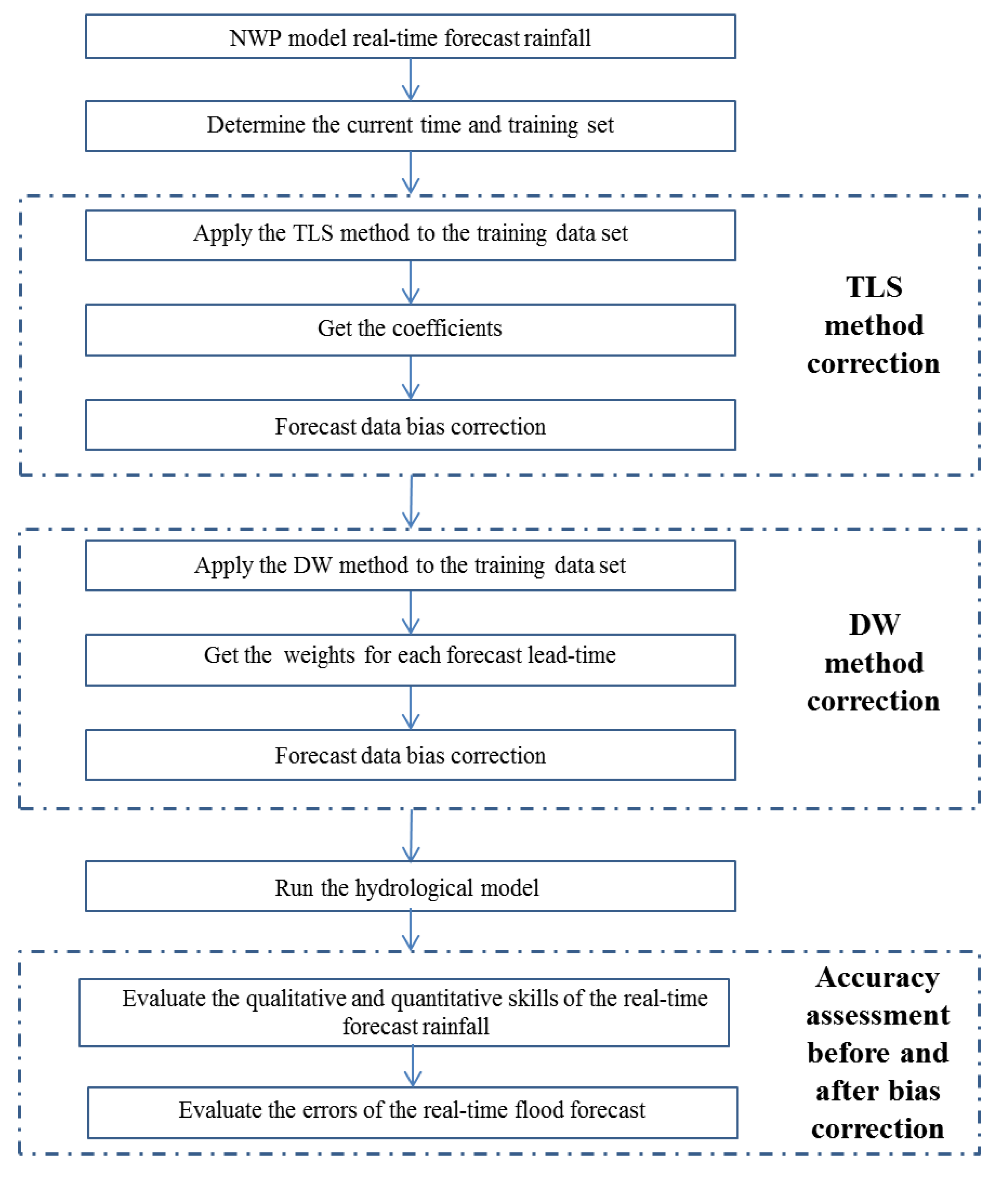
3.3. Real-Time Forecast Data Post-Processing

In the current research, real-time forecast meteorological data were produced using the WRF model. The WRF model biases, which led to the inaccuracy of the raw forecast data, were improved by applying the post-processing methods. The TLS and DW methods were applied to correct the biases of the real-time meteorological data, taking into consideration the bias lead-time dependency in the WRF forecast data. The criteria for the bias correction of the WRF data were defined based on removing the biases of the real-time forecast data, which are lead-time dependent. The challenge for real-time forecast correction is to choose an appropriate training data set. For this study, it requires at least a 72 h training period, which is necessary for obtaining the correction coefficients for the TLS and DW methods. For parameter estimation using TLS and DW, a training period of 72 h was selected to obtain the bias correction factor for different lead-times. The structure of the 72 h forecast data and choice of the current time for the bias correction are shown in Figure 2.

To obtain the bias correction coefficients, the first 72 h from the first ensemble—with 66 h from the next ensemble and 6 h from the last ensemble—was chosen for the current time. Using the data in the training set, the coefficients were obtained by applying the TLS and DW methods. Then, they were used to correct the forecast data. The objective of the OLS method is to obtain the parameters, which are the slope and a constant for the best fit line; however, in TLS, the residual is calculated via a different method. The difference between OSL and TLS is visually shown in Figure 3. The OLS method is one of the most popular methods of linear fitting. The OLS cost function F is the mean squares error of the observed and forecast data, which finds the best fit line to minimize the error (Equation (1)).

$$\mathrm{f}={\displaystyle \sum }_{i=1}^n{\epsilon }_{yi}^2$$

(1)

The TLS is similar to OLS, but instead of using vertical residuals, it uses diagonal residuals. The TLS was developed to modify the OLS, since it minimizes the cost function by utilizing the observed and forecast data (Equation (2)).

$$\mathrm{f}={\displaystyle \sum }_{i=1}^n\left({\epsilon }_{xi}^2+{\epsilon }_{yi}^2\right)$$

(2)

The TLS method is preferred over OLS, because in the OLS all the sample data are measured exactly without error. However, in actuality, the situation is different and there are observational errors. Thus, OLS may not be the ideal method whereas TLS can solve this problem by considering errors in both the independent and dependent variables.

The NWP models often have systematic biases and errors due to parameterization and the initialization of physical phenomena. Because the NWP models accuracy and performance changes by forecast lead-time, appropriate weighting is essential for forecast error reduction in bias correction methods. One of the common ways of achieving this, is to give equal weighting to all the lead-times in the post-processing of the forecast values. Since the forecast error is dependent on the forecast lead-time, equal weighting may increase the number of errors related to the inaccuracy for the higher forecast lead-times. Therefore, other unequal weighting methods, such as dynamic weighting are suggested. The dynamic weighting scheme may decrease the errors related to the forecast lead-time and improve the forecast accuracy in a better and more accurate way. The weights for each forecast lead-time can be obtained based on how well the model performed in the training data set. That is, the closer a model forecast value is to the observation data, the larger the weight assigned to the forecast lead-time. The mean absolute error (MAER) shows that the performance can be used to derive the weights for each forecast lead-time using Equation (3):

$$d{w}_{i,j}=\frac{P_{i,j}^{-1}}{{{\displaystyle \sum }}_{i=1}^n{P}_{i,j}^{-1}}$$

(3)

where $d{w}_{i,j}$ is the weight for each forecast lead-time i of the sub-basin j, and is conversely related to the performance measure, $P_{i,j}$. The $d{w}_{i,j}$ is calculated at each lead-time to generate the proper weights for the bias correction. $P_{i,j}$ is calculated based on the MAER of lead-time i from sub-basin j by Equation (4):

$$P_{i,j}=\frac{1}{N}{\displaystyle \sum }_{i=1}^N\left|F_{i,j}-O_{i,j}\right|$$

(4)

where $F_{i,j}$ is the forecast at lead-time i from sub-basin j, and $O_{i,j}$ is the observation value at lead-time i from sub-basin j. In addition, N is the number of sub-basins for the comparison between the observed and forecast values for the different lead-times.

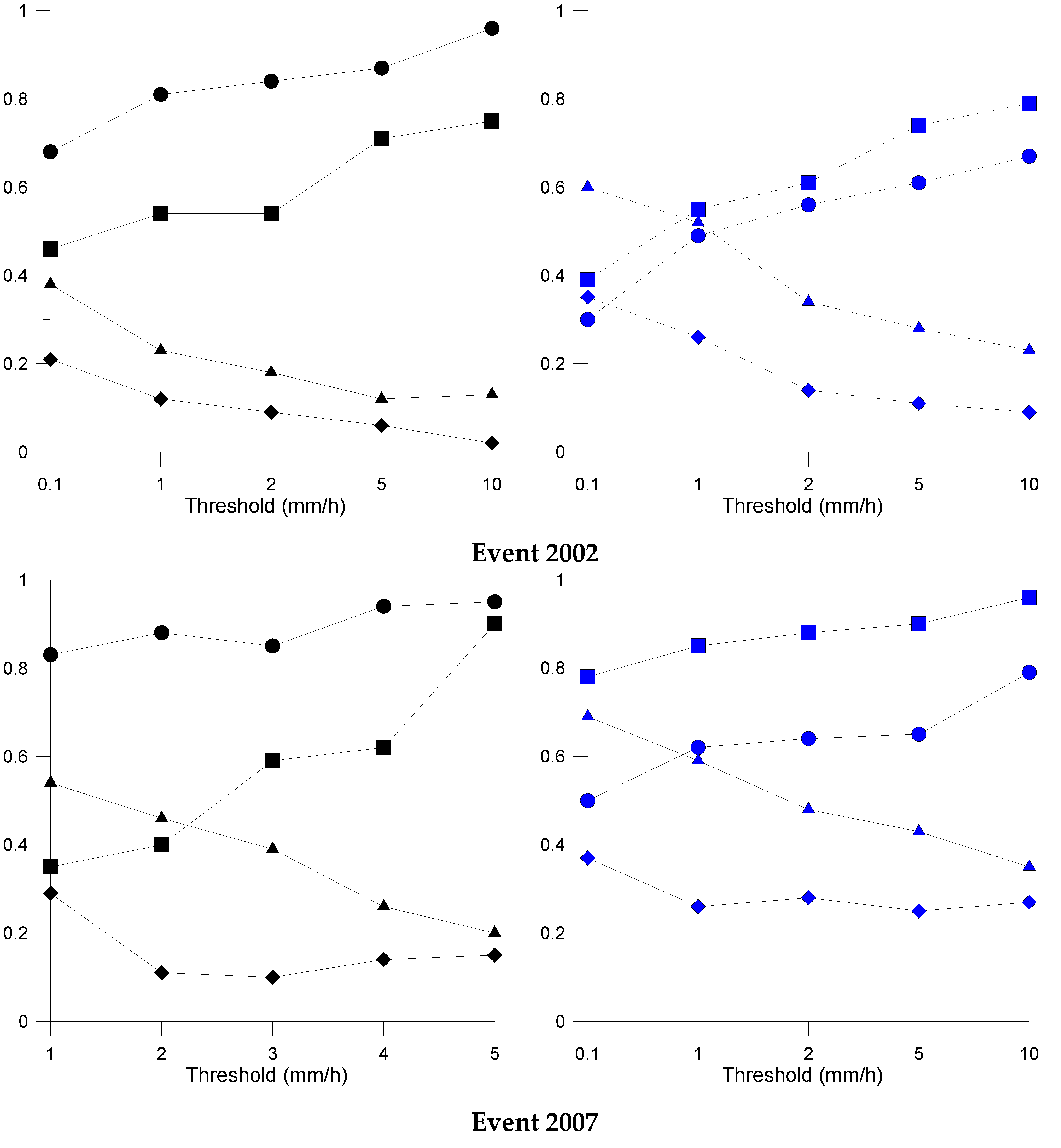
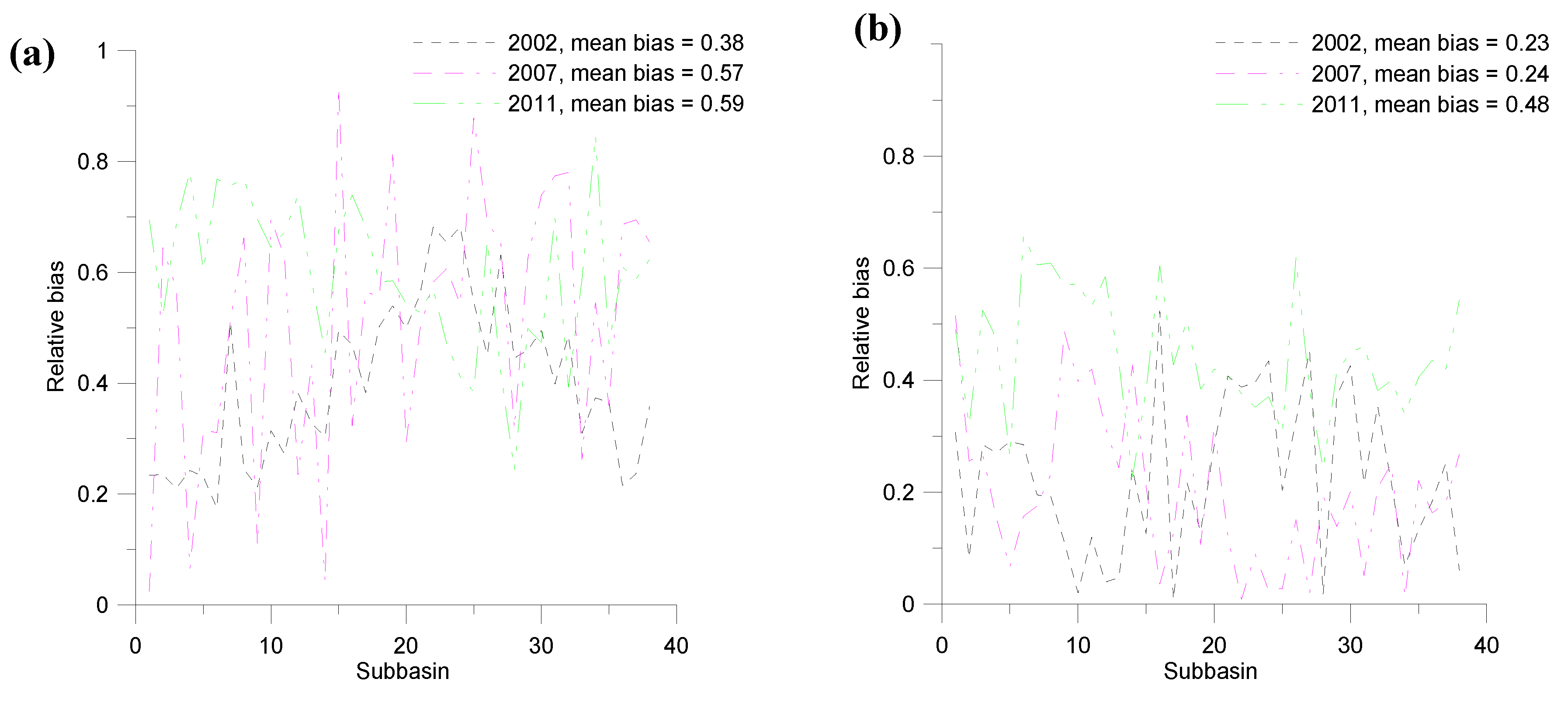
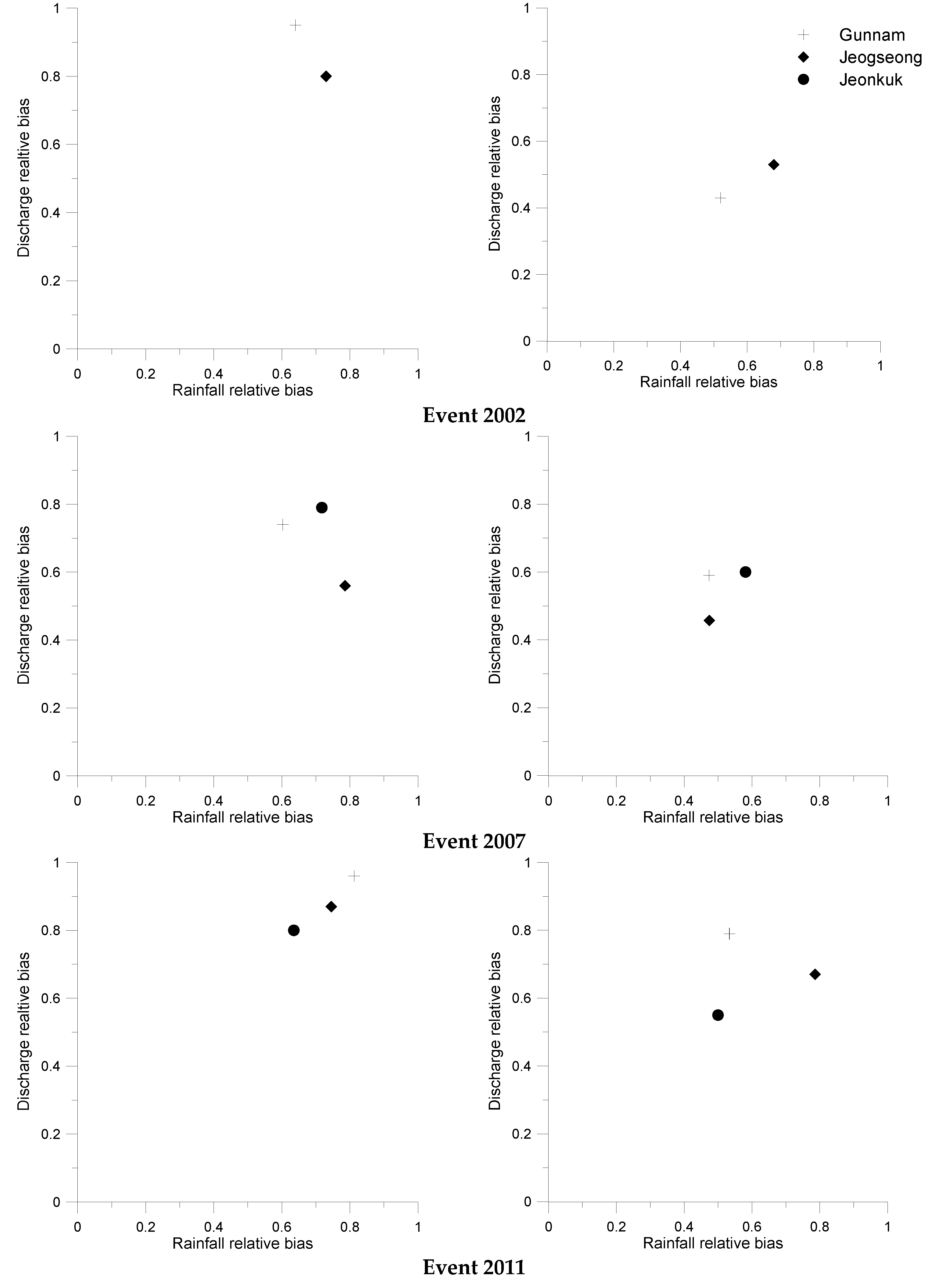
3.4. Accuracy Assessment

The steps of the suggested methods are summarized in Figure 4. This diagram includes the steps for the real-time data post-processing with the objective of improving the precipitation and flood forecast accuracy and the evaluation of the real-time forecast accuracy before and after applying the bias correction methods. In order to assess the performance of post-corrected real-time WRF precipitation, comparisons were made between the observed and forecast data. The forecast data can be verified using different verification methods, which are related to the forecast type of data and the verification aims. Overall, the forecast verification includes two main parts, the qualifying and quantifying analyses, which are shown in Appendix A.

4. Results and Analysis

The main goals of the post-processing methods are to increase the accuracy and readability of the biased raw forecast data. These goals can be addressed simultaneously by applying the bias correction methods for real-time data. The use of historical data and choosing the current time led us to find the error structure from the real-time WRF data. The application of the two bias correction methods—TLS and DW—simultaneously helped to find and reduce the systematic errors in the real-time data, which vary by increasing the lead-time. In the error evaluation of the real-time forecast rainfall, it is necessary to assess the WRF model’s ability to forecast rainfall occurrence as well as its amount.

The contingency table elements allow for visual identification of any differences (or not) between the observation and the raw/bias corrected real-time WRF data. The qualifying test is performed separately for five thresholds to obtain the bias scores for the real-time raw and post-processed forecast. The thresholds were chosen to discriminate between different rainfall intensities. The results of the qualifying analysis for the false alarm ratio (FAR), probability of detection (POD), percent correct (PC), and critical success index (CSI) for raw/bias corrected data are shown in Figure 5.

The forecasting ability of the WRF model decreased for higher rainfall thresholds, which is related to the challenges of correctly predicting the higher rainfall intensities when using NWP models. This demonstrated the necessity of applying the post-processing methods. According to Figure 5, the results indicated an error reduction for the different thresholds for the events of 2002, 2007 and 2011 after applying the post-processing methods. As can be seen, the post-processing approaches outperform the raw real-time forecast in terms of all scores by decreasing the FAR and increasing the POD, PC and CSI for all the data. The bias-corrected data performed better than the raw data as a result of the smaller number of false alarms and improved POD, PC and CSI values. The errors in the rainfall forecast in different sub-basins can be visually compared by plotting the relative bias errors for the bias corrected forecast and the raw data. The relative bias is used to evaluate the forecast precipitation accuracy and compared to the prediction performance of the bias-adjusted against non-adjusted real-time forecast data. The bias correction using TLS finds the bias structure between the raw forecast data and observed data, and the DW method is a bias detector, based on the different forecast lead times. Results of the precipitation bias assessment before and after applying the TLS and DW post-processing methods are shown in Figure 6. It is shown that the post-processing methods consistently improved the raw forecast data by keeping the accuracy high, as the forecast data were similar to those of the observed data.

In order to evaluate the effect of the TLS and DW methods on the real-time forecast data, the normalized error is utilized to compare the maximum observed and real-time raw/bias adjusted forecast data (

Table 1. The normalized error comparison between raw and bias corrected weather research and forecasting (WRF) for the events of 2002, 2007 and 2011.

Sub-basin	Event 2002			Event 2007			Event 2011
	Raw WRF	Revised WRF	Improvement (%)	Raw WRF	Revised WRF	Improvement (%)	Raw WRF	Revised WRF	Improvement (%)
1	0.84	0.40	52.94	0.91	0.79	12.85	0.27	0.95	71.87
2	0.84	0.12	86.03	0.83	0.06	93.19	0.67	0.84	20.29
3	0.84	0.12	85.64	0.81	0.07	91.42	0.70	0.80	12.61
4	0.86	0.32	62.42	0.87	0.22	74.96	0.42	0.80	46.89
5	0.85	0.30	64.57	0.92	0.59	35.54	0.55	0.82	33.27
6	0.88	0.49	43.92	0.92	0.58	37.35	0.24	0.84	71.64
7	0.58	0.44	24.51	0.90	0.59	34.69	0.57	0.79	28.76
8	0.85	0.28	67.06	0.93	0.55	40.57	0.53	0.80	34.44
9	0.88	0.43	51.45	0.88	0.35	59.84	0.28	0.78	64.65
10	0.85	0.11	86.86	0.84	0.33	60.47	0.61	0.79	22.56
11	0.86	0.21	75.79	0.96	0.60	37.05	0.13	0.67	80.03
12	0.89	0.26	70.28	0.91	0.47	48.29	0.68	0.85	20.40
13	0.83	0.02	97.30	0.90	0.21	76.23	0.91	0.70	30.58
14	0.83	0.20	75.66	0.95	0.45	52.25	0.30	0.71	57.50
15	0.87	0.37	57.64	0.81	0.12	85.73	0.42	0.55	24.16
16	0.87	0.17	79.98	0.92	0.33	64.48	0.67	0.85	21.57
17	0.85	0.03	96.58	0.92	0.44	52.57	0.08	0.69	88.89
18	0.89	0.30	66.64	0.83	0.18	78.16	0.35	0.80	56.08
19	0.86	0.11	86.93	0.93	0.56	40.09	0.45	0.73	37.95
20	0.91	0.42	53.49	0.90	0.41	54.82	0.30	0.67	55.21
21	0.89	0.35	61.44	0.91	0.56	39.02	0.45	0.71	36.39
22	0.93	0.35	62.30	0.93	0.73	21.24	0.42	0.77	46.09
23	0.89	0.11	88.10	0.85	0.34	59.26	0.66	0.80	16.92
24	0.90	0.24	72.97	0.86	0.09	89.02	0.48	0.68	29.65
25	0.90	0.10	88.44	0.89	0.62	30.37	0.42	0.72	41.93
26	0.85	0.15	81.82	0.88	0.61	30.52	0.47	0.73	35.70
27	0.89	0.25	71.60	0.86	0.54	37.20	0.14	0.63	77.21
28	0.85	0.06	92.40	0.88	0.03	96.53	0.21	0.42	49.00
29	0.87	0.29	65.95	0.90	0.49	45.29	0.37	0.72	48.65
30	0.86	0.27	68.00	0.82	0.57	30.69	0.36	0.69	47.21
31	0.85	0.19	77.67	0.91	0.60	34.10	0.29	0.71	58.39
32	0.87	0.25	71.15	0.86	0.69	19.32	0.51	0.81	36.91
33	0.86	0.28	67.01	0.95	0.70	26.83	0.53	0.75	29.59
34	0.87	0.05	94.62	0.94	0.72	23.20	0.61	0.79	22.56
35	0.85	0.14	83.67	0.93	0.62	33.12	0.44	0.75	41.50
36	0.84	0.27	68.13	0.91	0.67	25.58	0.03	0.72	96.43
37	0.87	0.43	50.58	0.89	0.52	41.50	0.30	0.73	59.75
38	0.87	0.12	86.23	0.89	0.50	43.78	0.31	0.76	59.50
Average	0.86	0.24	72.05	0.89	0.46	48.87	0.42	0.75	45.07

). The normalized error compares the errors relative to all sub-basins to give a general idea of the model’s performance, before and after applying the bias correction. In this part, the observed and raw/bias adjusted MAPs—which are the average of the precipitation over the entire sub-basin—are compared for the whole catchment.

By applying the post-processing methods, the real-time rainfall forecast error decreased and led to an increase in the QPFs performance in all the sub-basins. The TLS and DW methods improved the accuracy of the precipitation forecast by, on average, 72.05%, 48.87% and 45.07% for the events of 2002, 2007 and 2011, respectively. The SI performance measure was used to evaluate the results of applying the TLS and DW methods for the real-time forecast data. The results of the comparison between the raw and bias corrected precipitation data for the SI are shown in

Table 2. The scatter index comparison between the raw and bias corrected WRF for the events of 2002, 2007 and 2011.

Sub-basin	Event 2002			Event 2007			Event 2011
	Raw WRF	Revised WRF	Improvement (%)	Raw WRF	Revised WRF	Improvement (%)	Raw WRF	Revised WRF	Improvement (%)
1	3.55	3.00	18.48	4.87	4.08	19.26	2.32	1.84	26.03
2	3.87	3.00	28.92	5.00	3.70	35.17	2.37	1.31	81.24
3	4.58	3.01	52.44	6.79	4.19	62.22	2.01	1.03	94.22
4	3.47	2.89	20.06	4.79	3.91	22.53	1.86	1.31	42.43
5	3.53	3.00	17.79	5.05	4.39	15.12	2.77	1.46	89.83
6	3.80	3.32	14.65	4.47	4.18	6.82	1.98	1.07	84.95
7	3.81	2.23	70.81	4.67	4.14	12.95	2.19	1.17	87.66
8	3.67	2.99	22.67	5.35	4.51	18.69	2.17	1.17	84.88
9	4.03	3.31	21.99	5.92	3.89	52.39	2.18	1.30	68.49
10	3.76	2.64	42.70	5.29	4.82	9.71	2.02	1.62	25.10
11	3.80	2.99	27.23	5.35	4.36	22.84	1.64	1.26	29.94
12	3.79	2.81	34.85	5.49	4.31	27.34	2.25	1.27	77.78
13	3.84	2.64	45.74	4.79	3.70	29.28	2.32	1.88	23.63
14	3.39	2.71	24.92	5.48	4.15	32.26	2.18	1.69	28.98
15	3.71	2.87	29.13	6.14	4.14	48.46	1.89	1.32	42.88
16	4.85	2.57	88.92	4.06	3.49	16.03	2.04	1.41	45.28
17	3.74	2.72	37.34	4.64	4.04	14.83	2.05	1.61	26.89
18	3.20	2.45	30.79	4.74	3.78	25.48	2.19	1.75	25.05
19	3.37	2.45	37.29	4.84	4.53	6.91	2.39	1.03	132.93
20	3.18	2.62	21.50	5.53	4.21	31.54	2.22	1.77	25.06
21	3.04	2.65	14.77	4.58	4.29	6.78	2.39	1.91	24.71
22	3.08	2.72	13.16	5.13	4.94	3.84	2.57	1.43	79.25
23	2.82	2.42	16.72	4.20	4.03	4.34	2.36	1.93	22.27
24	2.75	2.39	15.13	3.88	3.23	20.19	2.16	1.17	84.12
25	3.17	2.38	33.08	4.95	4.51	9.71	2.28	1.84	24.04
26	3.07	2.50	22.65	4.68	3.06	52.87	2.49	1.75	41.82
27	2.77	2.41	14.94	4.15	4.14	0.29	2.15	1.40	53.18
28	3.68	2.49	47.56	4.09	3.32	23.23	2.15	1.17	84.38
29	3.07	2.59	18.73	4.07	3.84	5.75	2.30	1.45	58.13
30	2.92	2.50	16.73	4.16	3.37	23.49	2.42	1.94	24.39
31	3.30	2.55	29.36	4.38	2.30	90.40	2.29	1.83	25.48
32	3.06	2.55	19.92	4.70	2.62	79.76	2.56	1.73	47.35
33	3.32	2.68	23.96	4.74	3.60	31.49	2.63	1.64	60.29
34	3.46	2.49	39.32	5.06	4.78	5.74	2.55	1.62	57.53
35	3.31	2.47	33.80	4.33	4.18	3.57	2.42	1.98	21.97
36	3.46	2.78	24.67	4.37	2.34	86.58	2.33	1.28	82.00
37	3.47	2.88	20.41	4.01	3.99	0.59	2.28	1.36	67.94
38	3.50	2.58	35.76	5.62	5.11	10.09	2.36	1.94	21.09
Average	3.48	2.69	29.71	4.85	3.95	25.49	2.26	1.52	53.24

.

Applying the error correction methods improved the accuracy of the real-time precipitation data across all the events. The results indicated that by applying the bias correction methods, the SI performance measure improved by 29.71%, 25.49% and 53.24% for the events in 2002, 2007 and 2011, respectively. The findings showed that it is vital to use the two bias correction methods to improve the reliability and accuracy of the real-time forecast data.

In this study, the streamflow is forecast using the precipitation forecasts in the SURR model. The real-time forecasts of both precipitation and discharge over the Imjin River basin were evaluated and the verification was performed for the Gunnam, Jeogseong and Jeonkuk hydrological stations. The bias assessments of the precipitation and discharge are shown in Figure 7 for the Gunnam, Jeonkuk and Jeogseong stations before and after post-processing. This figure shows a comparison between precipitation and flood forecast errors based on relative bias error, and present the relationship between flood error and the precipitation forecast error. The post-processing methods, including the TLS and DW methods, were proven to substantially reduce the biases of real-time forecast precipitation when compared to observed data sets. Furthermore, the findings indicate that the error in the real-time discharge evaluation is higher than the error in the precipitation, which is obvious for all three hydrological stations.

The performance of the flood forecast is evaluated and compared using the observed streamflow, in order to show how biases in forecast precipitation lead to inadequate streamflow forecasting. The error propagation in the Gunnam, Jeonkuk and Jeogseong stations are shown in Figure 8.

After applying the bias correction methods, the streamflow forecasts were better matched with the corresponding observed data. The results showed a reduction in errors and an improvement in accuracy in all the stations across the 2002, 2007 and 2011 events. On average, the error was reduced by 78.58%, 81.26% and 62.33% for the events in 2002, 2007 and 2011, respectively. The Kling–Gupta efficiency (KGE) was used to compare the performance of the raw and bias corrected hydrological simulations and forecasts. After applying the TLS and DW bias correction methods, the results of the flood forecasts improved significantly (

Table 3. The comparison of the Kling–Gupta efficiency (KGE) measurement before and after bias correction for events in 2002, 2007 and 2011.

Index.	Station	SURR	SURR-WRF	SURR-Revised WRF
			Event 2002
KGE	Gunnam	0.41	−1.20	0.33
KGE	Jeogseong	0.60	−1.14	0.29
			Event 2007
KGE	Gunnam	0.53	−5.03	0.34
KGE	Jeonkuk	0.62	−2.77	0.27
KGE	Jeogseong	0.51	−3.30	0.23
			Event 2011
KGE	Gunnam	0.81	−0.26	0.40
KGE	Jeonkuk	0.60	−0.79	0.31
KGE	Jeogseong	0.81	−1.22	0.24

).

A comparison between the observed and forecast MAP and streamflow shows the efficiency of the TLS and DW post-processing methods. The flood forecast accuracy measurement was performed to show the ability of the coupled models to produce forecasts. Therefore, the prediction accuracy was assessed by comparing the observed, simulated and forecasted data. The simulation floods were estimated using the observed MAP as inputs to the SURR model, while the forecasts were obtained using the real-time WRF data as the input to run the SURR model. In this study, we used gauge and WRF precipitation to drive the hydrological model to simulate and forecast the flood events. The 72 h real-time forecast data were used as inputs to the SURR model over the Imjin River basin, and the bias corrected WRF data were also used as the input data for the SURR model. Due to space limitations, only one streamflow forecast is shown with the relevant precipitation. Applying bias correction to the precipitation simulation led to a reduction in the forecast hydrograph’s errors. Accordingly, the accuracy of the real-time flood forecast can be improved. Applying the TLS and DW methods improved the real-time precipitation and flood forecast for all the events in the Imjin River basin. The time series of the observed, simulated, forecasted, and bias corrected forecast streamflow data, along with the MAPs are shown in Figure 9. It should be noted that there is no observed data for Jeonkuk station in 2002.

Applying the TLS and DW methods improved the accuracy of the results for MAPs and floods in the Gunnam, Jeonkuk and Jeogseong stations for the events in 2002, 2007 and 2011. After applying the bias correction methods, the real-time forecast data improved by reducing the biases in the raw WRF data and improving the estimation of the raw WRF data in all stations and events.

5. Discussion

The errors produced by NWP models are typically related to the model parametrization, and the initial and boundary conditions. Although the initial and boundary conditions and model parametrizations have improved over time, NWP models have uncertainties that lead to imperfect rainfall forecasts. As a result, the real-time forecast precipitation is significantly different to the corresponding observed rainfall. Furthermore, increasing the forecast lead-time, also increases the forecast errors.

Uncertainties related to NWP real-time rainfall forecasts can have significant impacts on real-time hydrologic forecasts. Therefore, these errors should be assessed and reduced by post-processing methods to prevent error propagation in the flood forecast. Despite the significant impact of forecast errors on flood forecasting, few studies have determined how NWP errors propagate in hydrological model forecasts. In particular, bias correction of the real-time flood forecasting and the effects of forecast lead-time on the biases have not been addressed in this context. Therefore, post-processing methods—especially those that consider the bias lead-time dependency—are necessary.

The aim of the study was to investigate the application of two post-processing methods—namely, the TLS and DW methods—which consider the effects of forecast lead-time on the real-time bias of WRF model data. The reason for choosing these methods is that the TLS is a good alternative to the simple OLS method because it considers the potential bias correction in a more concise way. Furthermore, the forecast error is strongly dependent on the forecast lead-time and it is necessary to consider the bias lead-time dependency. To overcome this problem, the other bias correction method—the DW method—provides the lead-time dependent weights to the forecast members. The 72 h real-time forecast data of the WRF model underestimated the rainfall for all the events, which led to the underestimation of the real-time flood forecast in the studied area. The underestimation of the WRF model has also been reported in previous studies [28], which is in agreement with our current study. The application of the bias correction methods resulted in a more accurate rainfall forecast. Applying the TLS and DW methods and considering the effects of the lead-time-dependency on the real-time forecast data improved the WRF real-time forecast data, which led to an improvement in the real-time flood forecast.

In previous studies, different post-processing methods have been shown to improve the QPF alone, or have applied the improved QPF in the streamflow forecast. Reproducing the QPF by relating the observed precipitation and QPF using the Bayesian joint probability (BJP) modeling approach and the Schaake shuffle resulted in smaller forecast errors than that of the raw QPFs [10]. In the current study, using statistical bias correction (TLS and DW), which is an alternative to regenerating the ensemble forecasts, improved the accuracy of the real-time forecast.

A comparison of the real-time forecast data before and after applying the bias correction methods showed that the real-time forecast was more accurate after bias correction. However, the perfect match between the real-time flood forecast and observed streamflow in the studied catchment is challenging due to two reasons. First, the real-time forecast and observed precipitation are different sources of precipitation, and applying bias correction methods can somehow improve the raw forecast data. Secondly, the real-time flood forecast uncertainty is also due to the hydrological model calibration and verification because these models are often calibrated and verified using the observed precipitation while the real-time forecast rainfall is used to obtain the real-time flood forecast. The various sources of the inputs into the hydrological model led to different hydrological responses for forecasting the streamflow. Although the real-time flood forecasts do not perfectly match the observations, the available forecast data are still preferred due to the importance of the study area to North and South Korea, and obtainable information regarding flash floods and real-time flood forecasts is worthy of analysis.

6. Conclusions

The WRF model underestimated the real-time rainfall when compared with the observed data. The TLS bias correction method provides the bias structure between the raw forecast data and observed data, and the DW method is a bias detector based on different forecast lead times. By applying the bias correction method, the real-time forecast data improved significantly. The results of testing showed that the WRF model was less accurate for higher rainfall thresholds. Applying the bias correction methods improved the FAR, POD, PC and CSI for all the events studied. The TLS and DW methods improved the accuracy of the precipitation by decreasing the normalized error by, on average, 72.05%, 48.87% and 45.07%, and the SI improved by 29.71%, 25.49% and 53.24% for the events in 2002, 2007 and 2011, respectively. The comparison between the real-time precipitation and flood forecast relative bias error showed that applying the TLS and DW methods reduced the biases of the real-time forecast precipitation when compared to the observed streamflow. The results of the real-time flood forecast assessment showed error reductions and accuracy improvements of 78.58%, 81.26% and 62.33% in the 2002, 2007 and 2011 events, respectively. The KGE statistical measurement showed the flood forecast accuracy improvement in the Gunnam, Jeonkuk and Jeogseong stations for the events in 2002, 2007 and 2011. In a time-series analysis, applying the post-processing TLS and DW methods improved the accuracy of the flood forecast and MAPs in the Gunnam, Jeonkuk and Jeogseong stations by decreasing the underestimation of the real-time WRF data in the 2002, 2007 and 2011 events.

References

1. Robertson, D.E.; Shrestha, D.L.; Wang, Q.J. Post-processing rainfall forecasts from numerical weather prediction models for short-term streamflow forecasting. Hydrol. Earth Syst. Sci. Discuss. 2013, 17, 3587–3603. [Google Scholar] [CrossRef] [Green Version]
2. Jha, S.K.; Shrestha, D.L.; Stadnyk, T.; Coulibaly, P. Evaluation of ensemble precipitation forecasts generated through postprocessing in a Canadian catchment. Hydrol. Earth Syst. Sci. Discuss. 2018, 22, 1957–1969. [Google Scholar] [CrossRef] [Green Version]
3. Yucel, I.; Onen, A.; Yilmaz, K.K.; Gochis, D.J. Calibration and evaluation of a flood forecasting system: Utility of numerical weather prediction model, data assimilation and satellite-based rainfall. J. Hydrol. 2015, 523, 49–66. [Google Scholar] [CrossRef] [Green Version]
4. Cloke, H.L.; Pappenberger, F. Ensemble flood forecasting: A review. J. Hydrol. 2009, 375, 613–626. [Google Scholar] [CrossRef]
5. Jee, J.B.; Kim, S. Sensitivity Study on High-Resolution WRF Precipitation Forecast for a Heavy Rainfall Event. Atmosphere 2017, 8, 96. [Google Scholar] [CrossRef] [Green Version]
6. Wang, X.; Steinle, P.; Seed, A.; Xiao, Y. The Sensitivity of Heavy Precipitation to Horizontal Resolution, Domain Size, and Rain Rate Assimilation: Case Studies with a Convection-Permitting Model. Adv. Meteorol. 2016, 2016, 7943845. [Google Scholar] [CrossRef]
7. Goswami, P.; Shivappa, H.; Goud, S. Comparative analysis of the role of domain size, horizontal resolution and initial conditions in the simulation of tropical heavy rainfall events. Meteorol. Appl. 2012, 19, 170–178. [Google Scholar] [CrossRef]
8. Calvetti, L.; Pereira, F.A.J. Ensemble hydrometeorological forecasts using WRF hourly QPF and TopModel for a middle watershed. Adv. Meteorol. 2014, 2014, 484120. [Google Scholar] [CrossRef] [Green Version]
9. Pappenberger, F.; Beven, K.J.; Hunter, N.; Bates, P.D.; Gouweleeuw, B.; Thielen, J.; DeRoo, A.P.J. Cascading model uncertainty from medium range weather forecasts (10 days) through a rainfall–runoff model to flood inundation predictions within the European Flood Forecasting System (EFFS). Hydrol. Earth Syst. Sci. Discuss. 2005, 9, 381–393. [Google Scholar] [CrossRef] [Green Version]
10. Shrestha, D.L.; Robertson, D.E.; Bennett, J.C.; Wang, Q.J. Improving precipitation forecasts by generating ensembles through postprocessing. Mon. Weather Rev. 2015, 143, 3642–3663. [Google Scholar] [CrossRef]
11. Carlberg, B.R.; Gallus, W.A., Jr.; Franz, K.J. A preliminary examination of WRF ensemble prediction of convective mode evolution. Weather Forecast. 2018, 33, 783–798. [Google Scholar] [CrossRef]
12. Bhuiyan, M.A.E.; Nikolopoulos, E.I.; Anagnostou, E.N.; Quintana-Seguí, P.; Barella-Ortiz, A. A Nonparametric Statistical Technique for Combining Global Precipitation Datasets: Development and Hydrological Evaluation over the Iberian Peninsula. Hydrol. Earth Syst. Sci. Discuss. 2018. [Google Scholar] [CrossRef] [Green Version]
13. Nguyen, H.M.; Bae, D.H. An approach for improving the capability of a coupled meteorological and hydrological model for rainfall and flood forecasts. J. Hydrol. 2019, 577, 124014. [Google Scholar] [CrossRef]
14. Sikder, M.S.; Hossain, F. Improving operational flood forecasting in monsoon climates with bias corrected quantitative forecasting of precipitation. Int. J. River Basin Manag. 2019, 17, 411–421. [Google Scholar] [CrossRef]
15. Cuo, L.; Pagano, T.C.; Wang, Q. A review of quantitative precipitation forecasts and their use in short to medium range streamflow forecasting. J. Hydrometeorol. 2018, 12, 713–728. [Google Scholar] [CrossRef]
16. Gao, S.; Huang, D. Assimilating Conventional and Doppler Radar Data with a Hybrid Approach to Improve Forecasting of a Convective System. Atmosphere 2017, 8, 188. [Google Scholar] [CrossRef] [Green Version]
17. Sloughter, J.M.; Raftery, A.E.; Gneiting, T.; Fraley, C. Probabilistic quantitative precipitation forecasting using Bayesian model averaging. Mon. Weather Rev. 2007, 135, 3209–3220. [Google Scholar] [CrossRef]
18. Jabbari, A.; Bae, D.H. Application of Artificial Neural Networks for Accuracy Enhancements of Real-Time Flood Forecasting in the Imjin Basin. Water 2018, 10, 1626. [Google Scholar] [CrossRef] [Green Version]
19. Rogelis, M.C.; Werner, M. Streamflow forecasts from WRF precipitation for flood early warning in mountain tropical areas. Hydrol. Earth Syst. Sci. Discuss. 2017, 1–32. [Google Scholar] [CrossRef] [Green Version]
20. Yoon, S.S. Adaptive Blending Method of Radar-Based and Numerical Weather Prediction QPFs for Urban Flood Forecasting. Remote Sens. 2019, 11, 642. [Google Scholar] [CrossRef] [Green Version]
21. Li, J.; Pollinger, F.; Panitz, H.J.; Feldmann, H.; Paeth, H. Bias adjustment for decadal predictions of precipitation in Europe from CCLM. Clim. Dyn. 2019, 1–18. [Google Scholar] [CrossRef]
22. Lee, S.; Bae, D.H.; Cho, C.H. Changes in future precipitation over South Korea using a global high-resolution climate model. Asia Pac. J. Atmos. Sci. 2013, 49, 619–624. [Google Scholar] [CrossRef]
23. Jabbari, A.; So, J.-M.; Bae, D.-H. Precipitation Forecast Contribution Assessment in the Coupled Meteo-Hydrological Models. Atmosphere 2020, 11, 34. [Google Scholar] [CrossRef] [Green Version]
24. Skamarock, W.C.; Klemp, J.B. A time-split non-hydrostatic atmospheric model for weather research and forecasting applications. J. Comp. Phys. 2008, 227, 3465–3485. [Google Scholar] [CrossRef]
25. Bae, D.H.; Lee, B.J. Development of Continuous Rainfall Runoff Model for Flood Forecasting on the Large Scale Basin. J. Korea Water Resour. Assoc. 2011, 44, 51–64. [Google Scholar] [CrossRef]
26. Hong, S.-Y. Comparison of heavy rainfall mechanisms in Korea and the central US. J. Meteorol. Soc. Jpn. 2004, 82, 1469–1479. [Google Scholar] [CrossRef] [Green Version]
27. Song, H.-J.; Sohn, B.-J. An Evaluation of WRF microphysics Schemes for Simulating the Warm-Type Heavy Rain over the Korean Peninsula. Asia Pac. J. Atmos. Sci. 2018, 54, 225–236. [Google Scholar] [CrossRef]
28. Chawla, I.; Osuri, K.K.; Mujumdar, P.P.; Niyogi, D. Assessment of the Weather Research and Forecasting (WRF) model for simulation of extreme rainfall events in the upper Ganga Basin. Hydrol. Earth Syst. Sci. Discuss. 2018, 22, 1095–1117. [Google Scholar] [CrossRef] [Green Version]
Figure 1. (a) The digital elevation model (DEM) of the Imjin River basin, (b) the sub-basins, river network and water levels and (c) location of rain gauge stations in the Imjin River basin.
Atmosphere 11 00300 g001
Figure 2. The structure of the real-time forecast data and selection of the current time for applying the bias correction.
Atmosphere 11 00300 g002
Figure 3. A visual comparison between the ordinary least squares (OLS) and total least squares (TLS) methods.
Atmosphere 11 00300 g003
Figure 4. The real-time data post-processing steps for improving the precipitation and flood forecast.
Atmosphere 11 00300 g004
Figure 5. The performance of the real-time forecast rainfall for different thresholds before (left side) and after (right side) bias correction.
Atmosphere 11 00300 g005aAtmosphere 11 00300 g005b
Figure 6. Comparison of the relative bias for the events of 2002, 2007 and 2011 for (a) before bias correction and (b) after bias correction.
Atmosphere 11 00300 g006
Figure 7. Bias assessment of the precipitation and discharge in the Gunnam, Jeonkuk and Jeogseong stations for before (left panel) and after (right panel) bias correction.
Atmosphere 11 00300 g007
Figure 8. Error assessment in Gunnam, Jeonkuk and Jeogseong stations for the events of 2002, 2007 and 2011.
Atmosphere 11 00300 g008aAtmosphere 11 00300 g008b
Figure 9. Time series of the observed, simulated, forecast and bias corrected forecast streamflow along with the mean areal precipitation (MAP) in Gunnam, Jeonkuk and Jeogseong stations
Atmosphere 11 00300 g009aAtmosphere 11 00300 g009b