Warm Rain in Southern West Africa: A Case Study at Savè

Abstract

A warm-rain episode over southern West Africa is analyzed using unprecedented X-band radar observations from Savè, Benin and a Large-Eddy Simulation (LES) over a 240 × 240 km${}^2$ domain. While warm rain contributes to 1% of the total rainfall in the LES, its spatial extent accounts for 24% of the area covered by rainfall. Almost all the warm-rain cells tracked in the observation and the LES have a size between 2 and 10 km and a lifetime varying from 5 to 60 min. During the nighttime, warm-rain cells are caused by the dissipation of large deep-convection systems while during the daytime they are formed by the boundary-layer thermals. The vertical extension of the warm-rain cells is limited by vertical wind shear at their top. In the simulation, their top is 1.6 km higher with respect to the radar observations due to the large-scale environment given by wrong initial conditions. This study shows the challenge of simulating warm rain in southern West Africa, a key phenomenon during the little dry season.

1. Introduction

Rainfall types over West Africa range from shallow, warm-rain-producing cloud elements to mesoscale convective systems (MCSs). While it is now commonly known that MCSs account for the vast majority of rainfall in the Sahel (e.g., [1,2]), there is a lack of robust rainfall type statistics for the wetter and more populous region of southern West Africa (SWA) lying to the south of the Sahel. Among the rainfall types, warm rain formed by clouds composed only of liquid hydrometeors has been understudied in the past.

One reason is the small size of these shallow clouds, on the order of 1 km [3], which makes their observation from space a challenge. Generally, satellites do not allow an accurate estimation of warm-rain amounts. Indeed, rainfall estimations highly rely on passive microwave radiometers and infrared imagers, which are mainly sensitive to ice particles and high-cloud tops. Thus, warm rain associated with shallow clouds may be misclassified when the latter are attached to MCSs or in the case of multi-layer cloud systems (e.g., [3,4]). Furthermore, instantaneous snapshots are not sufficient to determine if the shallow clouds are in their terminal stage or if they are a transient stage of evolving deep convection [5]. This can lead to uncertainties in the warm-rain amount calculations. Using a 9-year climatology of Tropical Rainfall Measuring Mission (TRMM) precipitation radar measurements [3] estimated the contribution of warm rain to total rainfall. They found a contribution of 20% over tropical oceans where shallow clouds occur predominantly (e.g., [6,7]) and of 7.5% over land, where the warm-rain clouds are deeper [3,8]. Note that the probability of rain from warm clouds over land increases towards coastal areas as shown by [7] using 5-year Cloud-Aerosol Lidar with Orthogonal Polarization (CALIOP) data.

Over SWA, some recent efforts have been undertaken to shed more light on the distribution and regional importance of warm rain. Based on a 16-year TRMM precipitation radar observation, [9] estimated that warm rain contributes at least 2% to total annual rainfall at the immediate coastal region of SWA and that such warm rain events predominantly occur in July and August. [10] developed a SWA-calibrated method to delineate precipitating liquid clouds using the spatio-temporally high-resolution dataset of the Spinning Enhanced Visible and Infrared Imager (SEVIRI). They found a unimodal seasonal cycle of the occurrence frequency with a distinct peak in August, which corresponds well with the results in [9]. They further estimated warm rain frequency over SWA, and found it to be larger over the coastlines, from 5% in Nigeria to 15% in Liberia. Despite the likely small contribution to annual amounts, the larger precipitation frequency yielded by warm rain may be important for agriculture, in contrast to the intense MCS-like rainfall that can generate floods and runoff over dry soils. The latter is particularly important during the “little dry season”, observed from mid-July to mid-September along the SWA coast, sometimes associated with droughts [11]. This motivates a better understanding of warm rain.

Current operational numerical-weather prediction models and convection-permitting research models run with horizontal grid meshes in the range of 1–20 km. The development of the boundary layer and the transition from stratus to convective clouds is at best partly resolved by these models, but usually fully parameterized. Their ability to represent warm rain is thus limited. Large-Eddy Simulations (LESs) can explicitly resolve the most energetic eddies in the boundary layer. Therefore, they are expected to better represent the warm-rain clouds. Among the modeling studies devoted to shallow convective clouds (e.g., [12,13,14,15]), only the work by [14] gives estimates of warm rain contributions from shallow (3 km top) and congestus (7 km top) clouds; the contributions are 3.6% and 34%, respectively. Their analysis is based on a 10-day case transitioning from suppressed to active phases of the Madden–Julian Oscillation.

In this paper, we investigate warm rain in SWA during the field campaign of the Dynamics–Aerosol–Chemistry–Cloud Interactions in West Africa (DACCIWA) project [16]. This field campaign took place in summer 2016. Intensive ground and radiosonde measurements were performed from mid-June to the end of July 2016 at three supersites in SWA: Kumasi (Ghana), Savè (Benin), and Ile-Ife (Nigeria). Savè was instrumented with an X-band rain radar deployed by the Karlsruhe Institute of Technology (KIT) [17]. Also, a radiosonde campaign run parallel in Savè and Kumasi (see [18] for details). Here, we use observations gathered during the campaign and a LES to explore one warm-rain episode. The objectives of the paper are twofold. First, to present a set of unprecedented observations made at the Savè supersite. There, the most remarkable event of warm rain was found on 24 July 2016, it was observed during the night and early morning. This case yielded 1.6 mm, as measured by the distrometer and the rain gauge, roughly half of the warm rain in Savè during the whole campaign. Other notable warm-rain cases were the 21 and 25 June, and the 27 July 2016, responsible for 0.31, 0.42 and 0.36 mm, respectively. In total, 3 mm were yielded by warm rain during the campaign, which represented 1.35% of total rainfall in Savè. An added value of this study is the use of the X-band rain radar, as it collects information on the vertical structure of the warm-rain cells and allows a characterization of warm rain at high spatial and temporal resolution. Both the rain radar and the LES are used to characterize warm rain. The second objective is to determine the mechanisms involved in the development of precipitating ice-free clouds in SWA. The case is analyzed based on a 200-m resolution LES performed with the research model Meso-NH [19]. This grid spacing allows a reasonable representation of turbulent fluxes in the boundary layer and meets our need to simulate a large domain (240 × 240 km${}^2$) covering the X-band radar range. The study by [14] has proven to resolve shallow convection with this resolution.

Our methodology to explore this event relies on a comparison of the simulated warm-rain cells and those observed by the X-band radar. The detection of warm-rain cells that lie, by definition, below 4-km altitude, is based on the clustering of reflectivity fields to delimit a volume of precipitating hydrometeors. This allows the characterization of the warm-rain cells in terms of their size, spatial distribution and vertical development. Then, the warm-rain cells are tracked in time, and the lifetime of each track is computed. To the best of the authors’ knowledge, this is the first time that the size or lifetime of warm-rain cells over SWA are statistically quantified.

The paper is organized as follows: Section 2 describes the observational datasets employed to characterize warm rain, particularly the X-band radar and the Meso-NH simulation, and the analysis approach. The case study is presented in Section 3, and the contribution of warm rain to total rainfall in the model is calculated. In Section 4 we analyse the properties of the warm-rain cells for both the radar and the simulation. The vertical profiles of the atmosphere and how they explain the differences between the observed and simulated warm-rain cells are discussed in Section 5. The water content, equivalent potential temperature, turbulence kinetic energy and wind shear inside the warm-rain-producing clouds are also explored. Section 6 concludes the paper.

2. Data and Methods

2.1. Observations from Savè Supersite

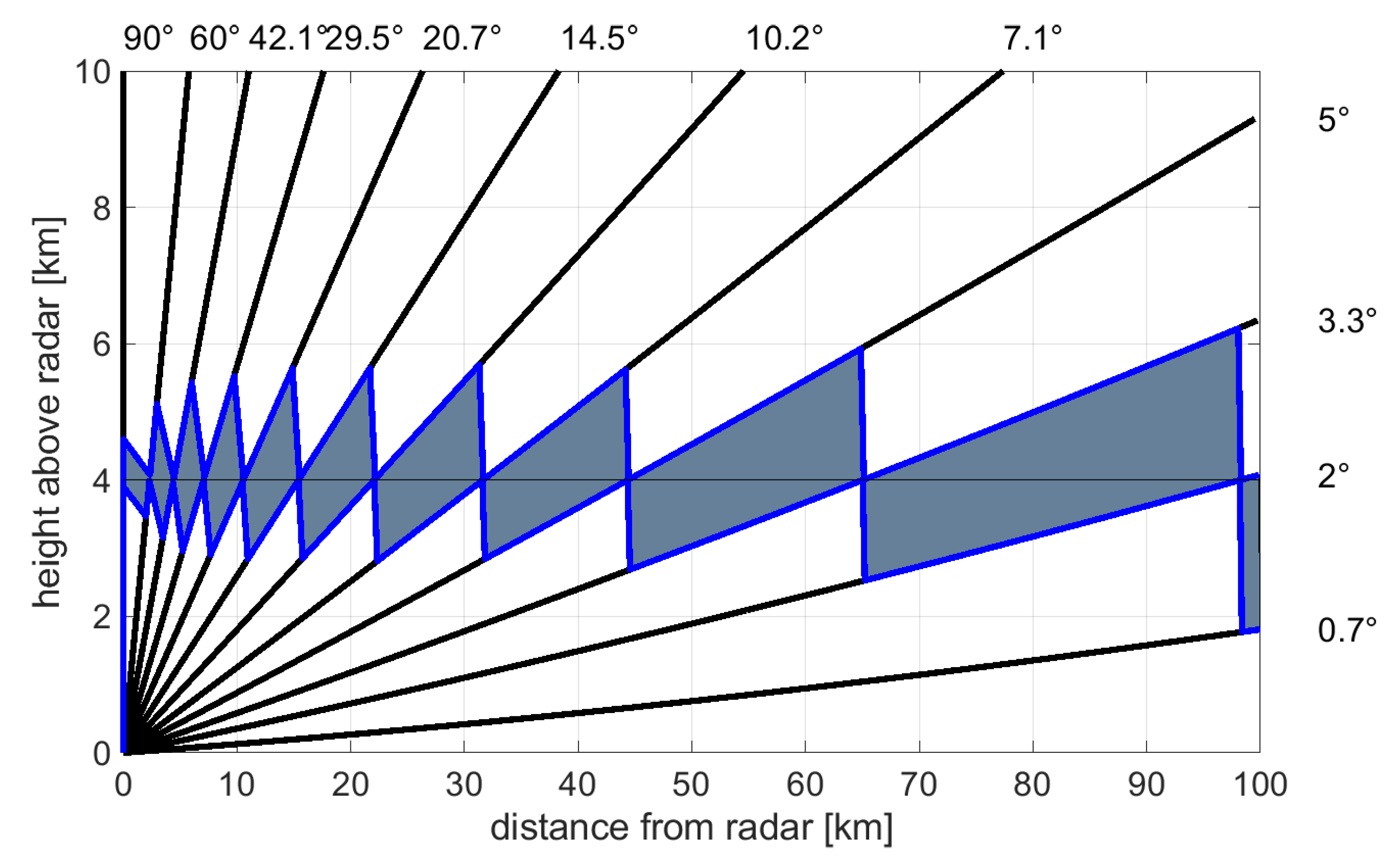
Warm-rain cells are defined in terms of reflectivities measured by the X-band radar at Savè (8.00${}^{\circ }$ N, 2.43${}^{\circ }$ E), in Benin. The radar is located at 183 m altitude. It is a Meteor50DX radar emitting at a frequency of 9.37 GHz, or equivalently a wavelength of ∼3 cm, and its horizontal range is set to 100 km. The reflectivity data is available in a polar grid with 12 elevation angles ranging from 0.7${}^{\circ }$ to 90${}^{\circ }$ and a resolution of 500 m and 1${}^{\circ }$ in the radial and azimuth coordinates, respectively. To illustrate the radar scan strategy, Figure 1 shows the altitudes and distances scanned for each elevation angle at a constant azimuth. For example, the reflectivity at 4-km altitude is only measured at a certain distance for each elevation angle; the regions which are not scanned are shaded. The uncertainty in the estimation of the echo heights is inherent to the radar observation, and becomes larger as the distance from the radar increases. The whole volume comprising all azimuths is scanned every 5 min. A calibration factor (7 dBZ) is applied to the logarithmic reflectivities due to a systematic underestimation.

The Savè supersite also took advantage of radiosonde observations daily at 06:00 UTC providing profiles of the atmosphere up to the stratosphere; and of additional high-frequency boundary-layer soundings during the Intensive Observation Periods; Modem M10 meteorological radiosondes were used. For this study, we use the standard observation on 24 July 2016 at 06:00 UTC and two frequent observations at 03:30 and 08:00 UTC. These soundings serve to evaluate the simulated vertical structure of the lower atmosphere in Savè. The rain rate derived from a Joss-Waldvogel-Distrometer and the measurements of reflectivity at vertical incidence from a cloud radar are also used. Further details on the instrumentation of the Savè supersite and the measurements done are given in [17,18].

2.2. Meso-NH Large-Eddy Simulation

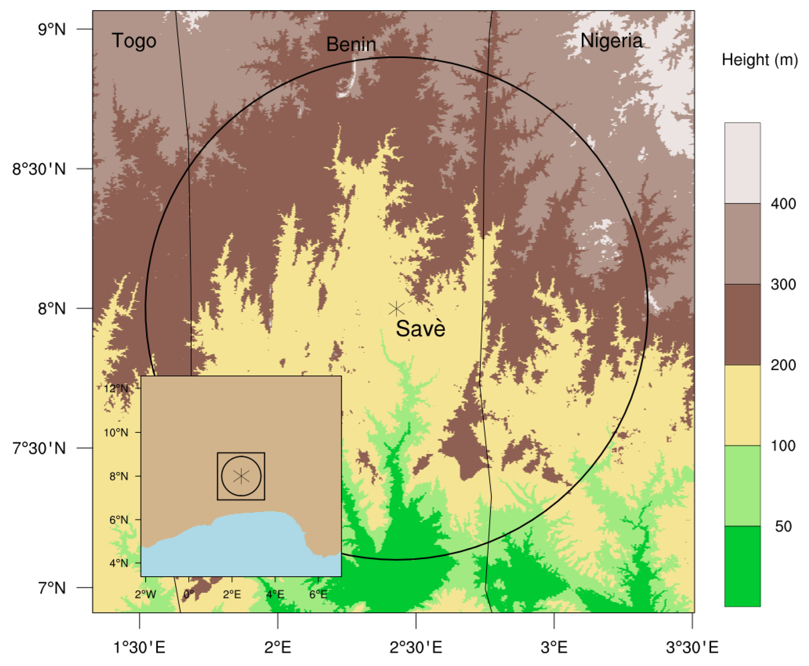
The non-hydrostatic mesoscale atmospheric Meso-NH model [19], version 5-4-0, is run with two nested grids with domains centred over the X-band radar location (Figure 2), using a one-way nesting method [20]. Meso-NH is run for 18 h on a large domain covering 1024 × 1024 km${}^2$ with a 1-km horizontal grid. It starts from ECMWF (European Centre for Medium-Range Weather Forecast) operational analysis at 18:00 UTC 23 July 2016. This initialization time allows one to simulate the nocturnal low-level jet (see [21] for a conceptual model of the nocturnal boundary layer in Savè). Boundary conditions are provided by ECMWF operational analysis at 00:00, 06:00 and 12:00 UTC 24 July 2016. Because the period of interest covers 03:00 to 08:00 UTC (see Section 3), the model is run for 10 h with a 200-m grid spacing over a 240 × 240 km${}^2$ domain, starting from the first run fields at 02:00 UTC 24 July 2016. Such a high resolution allows for the terrain, surface roughness and boundary-layer processes to be fairly represented. In this study, only the results from the 200-m simulation are analyzed and discussed. The vertical grid counts 64 levels up to 24-km altitude. A fine vertical spacing is set, varying from 40 to 200 m up to 5 km (approximately the height of the melting layer) in order to well resolve the processes in the edges of the warm-rain clouds. The vertical spacing stretches then up to ∼1 km above the tropopause. Output from the 200-m simulation is generated every 5 min, which is the X-band radar data frequency.

Both runs use the Surface Externalisée (SURFEX) scheme for surface fluxes [22], the Rapid Radiative Transfer Model [23] for longwave radiation and the two-stream scheme [24] for shortwave radiation. The 3-D turbulence scheme employed is a 1.5-order closure scheme [25] with the mixing length being the cubic root of the grid volume. A parameterization of dry thermals and shallow cumuli [26] and a subgrid statistical cloud scheme [27] are activated for the 1-km run while no shallow convection or subgrid cloud parameterizations are used for the 200-m run. We use a microphysical scheme for mixed-phase clouds [28]. In this scheme, the warm processes rely on the 1-moment Kessler scheme in which autoconversion of cloud water into rain is initiated beyond the critical cloud water content value of 0.5 g m${}^{-3}$. Finally, from the output of the 200-m simulation, reflectivities are computed in the Rayleigh approximation on each grid point of the model following [29].

2.3. Detection and Tracking of Warm-Rain Cells

Warm rain is detected every 5 min from 03:00 to 08:00 UTC. To ease the processing, the native polar grid of the radar reflectivities ($\Delta$r = 500 m) is transformed into a Cartesian grid with $\Delta$x = $\Delta$y = $\Delta$z = 500 m. For both the X-band radar observations and the simulation, the identification is done on the domain covering the radar range with a shared horizontal grid mesh of 1 km and the native vertical grid of each dataset. The method relies on the clustering algorithm developed by [30]. It consists of locating the grid points where a condition is verified, and grouping the contiguous points into a three-dimensional object, herein named warm-rain cell. To apply this algorithm, the 3-D reflectivities are first projected into the horizontal, such that the resulting fields correspond to the maximum values of reflectivity over the column. Then, a condition on the intensity of the maximum reflectivity is used to delimit the horizontal spread of the rain cells: it must be larger than 20 dBZ. Thresholds ranging from 18 to 20 dBZ are commonly used to identify light to moderate rain above 0.5 mm h${}^{-1}$ (e.g., [3,31,32,33]). 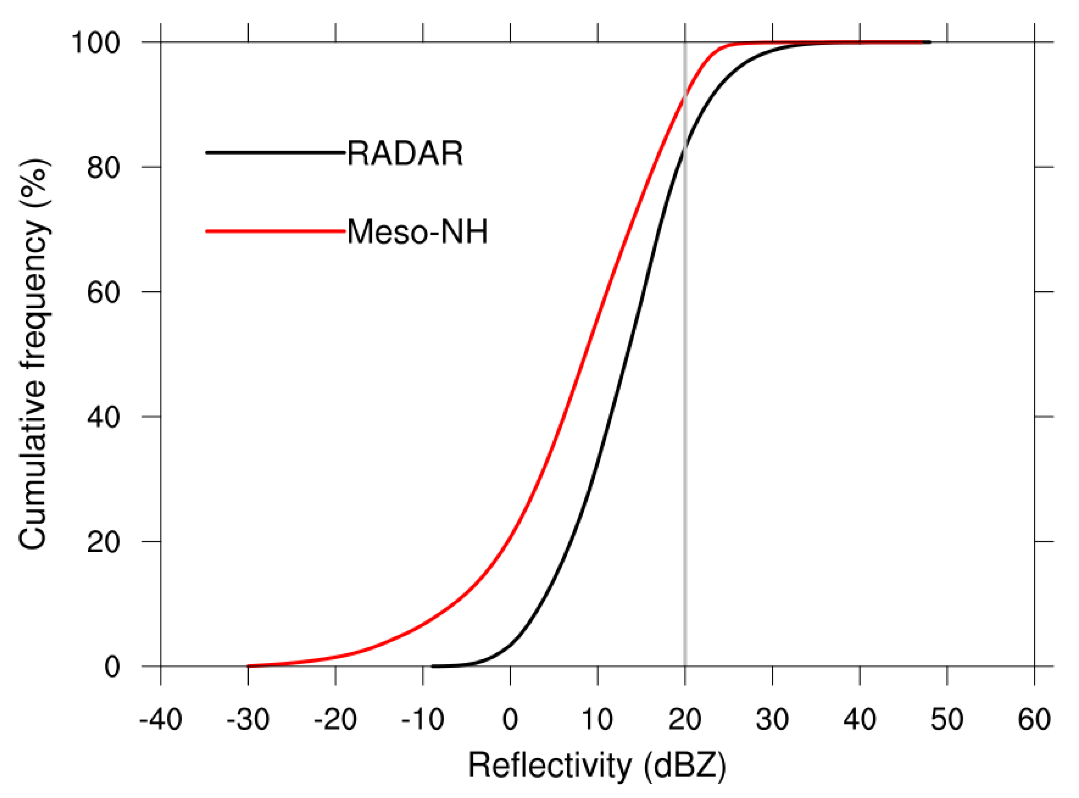Figure 3 shows the cumulative frequency distribution of the maximum reflectivity values to which the 20 dBZ threshold is applied, for the radar and model data. The distribution is shifted to lower values in the model with respect to the radar. While 16.9% of the observed reflectivity values exceed 20 dBZ, only 8.6% do in the simulation. A top is then associated with each identified cluster, defined as the highest altitude where a reflectivity of 20 dBZ is found inside the cluster for both datasets. A base is also computed as the lowest altitude where a reflectivity of 20 dBZ is found inside the cluster; but it is only done for the simulated rain cells. This is an added value of the simulation; it is not possible to compute the base height for the radar. Notice that, for the latter, the three first elevation angles are partially blocked by obstacles (e.g., bushes, buildings). The most severe blocking occurs for the first elevation angle (0.7${}^{\circ }$), with roughly 1/3 of the total area blocked, mainly covering the northeastern quadrant of the radar range. Each cluster with an effective diameter larger than 2 km (smaller clusters are considered as noise) and with the top located below 4 km is classified as a warm-rain cell. The effective diameter is defined as the diameter of a circle whose area equals the area covered by the cluster. We consider that this 4-km altitude corresponds to the freezing point temperature of 273 K in the clouds. 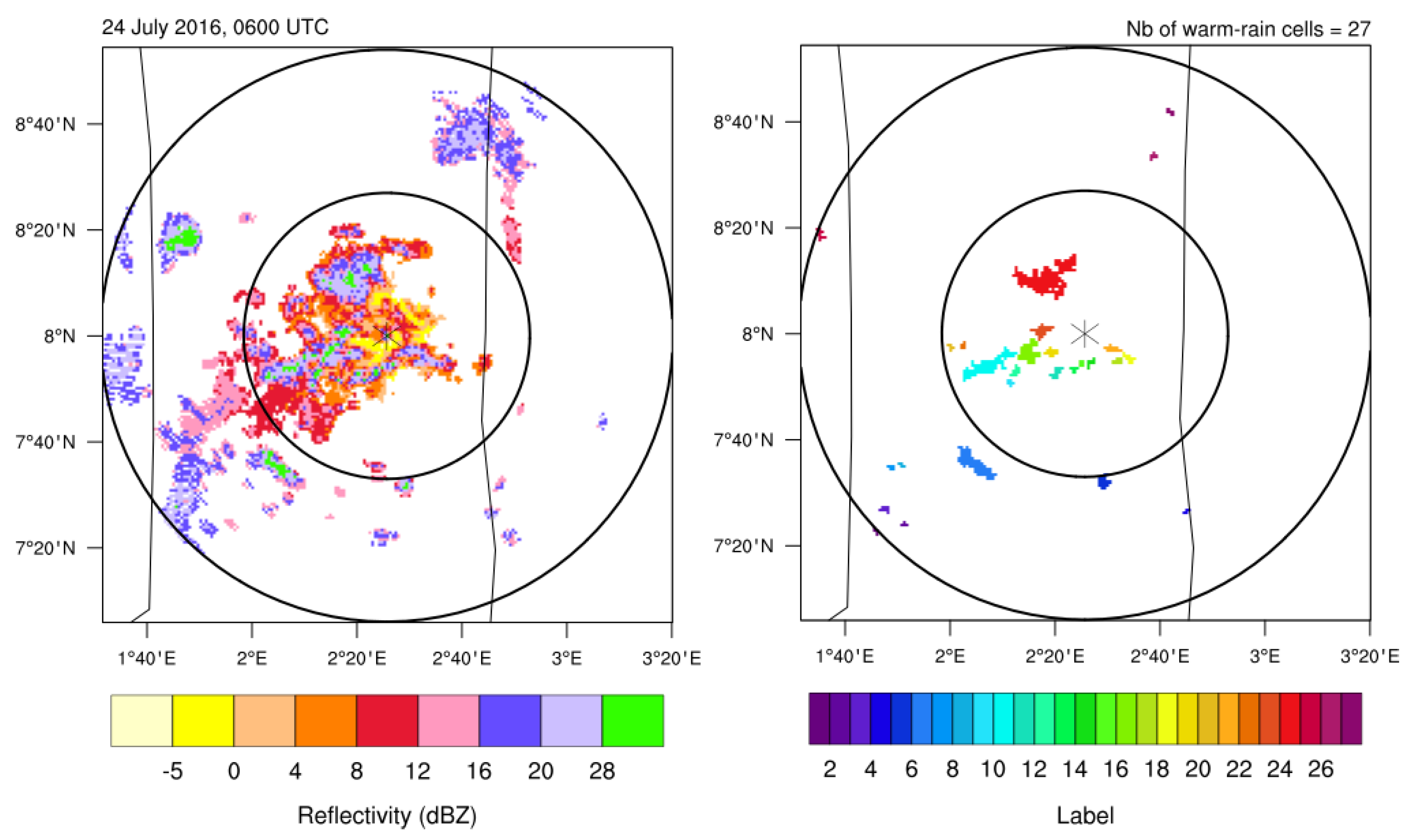It is, for instance, the same height that was used within TRMM to identify warm rain in the tropics by [6]. All the clouds with higher, thus colder tops cannot produce warm rain. Notwithstanding, in the clouds, it is very common to find supercooled water. In the absence of sufficiently precise data on this phenomenon, we decided to keep 4-km altitude threshold for warm rain, being aware of the limitation of this choice. To illustrate how the detection method is applied, Figure 4 shows a map of the reflectivity obtained from the X-band radar and the warm-rain cells identified at 06:00 UTC. The high-frequency of the detection method allows one to monitor the evolution of the number and characteristics of the cells, such as their size and lifetime, as will be shown in Section 4. Note that the lifetime of warm-rain cells should not be confused with that of warm clouds.

The simulated warm rain at ground is estimated for each cell based on the 5-min total accumulated rainfall maps. The rainfall gridpoints matching the individual cells are attributed to warm rain. As shown in Section 3, warm rain is accumulated over a 6-h period, from 03:00 to 09:00 UTC and over the entire model domain; the clustering algorithm for warm-rain cells is thus extended accordingly.

Finally, the tracking of warm-rain cells over time (developed by [30] to track deep-convective clouds) is done in a way that two warm-rain cells detected at two consecutive time steps are the same if the surface overlap between them is above a certain threshold; different thresholds are tested (see Section 4) and applied for both the observation and the LES.

3. Clouds and Rainfall

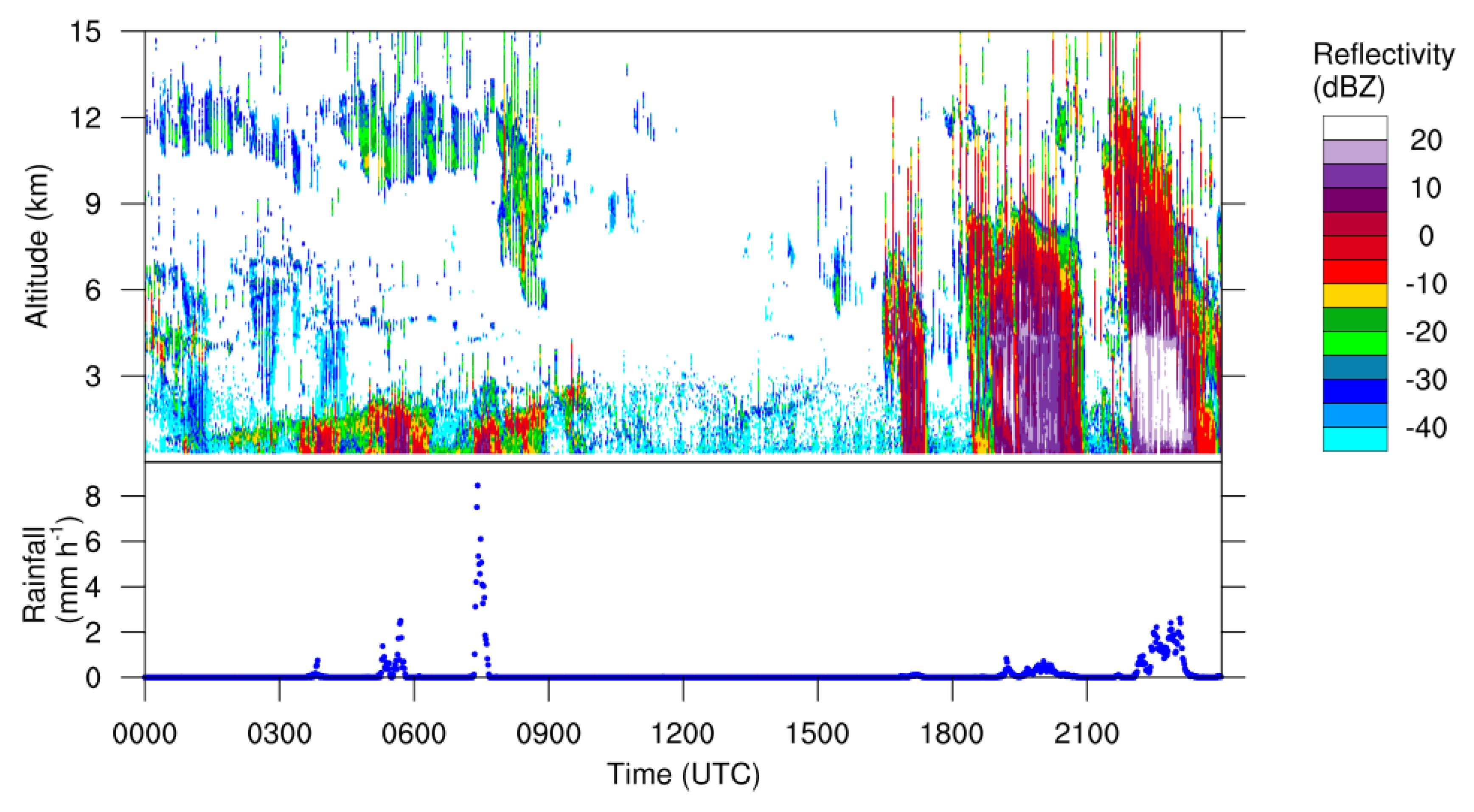
The vertical structure of clouds over Savè on 24 July 2016 is shown in Figure 5. During the night and early morning values of reflectivity larger than −10 dBZ are measured by the cloud radar below 2–3 km, corresponding to the presence of clouds. These clouds having tops below the freezing level are in liquid phase. Slightly before 04:00 UTC, from 05:00 to 06:00 UTC and at 07:30 UTC warm rain from these shallow clouds is measured by the distrometer, with intensities ranging from 1 to 9 mm h${}^{-1}$ (Figure 5, bottom). The warm rain amount is 1.6 mm, approximately half of the warm rain measured in Savè during the whole campaign from 19 June to 30 July 2016. This case and the three other warm rain cases observed during the field campaign yielded a total of 3 mm, which represents 1.35% of total rainfall in Savè. Deep-convective clouds develop in the afternoon and evening, reaching 8–10 km altitude before 21:00 UTC and up to 12 km after 21:00 UTC. In the following, our statistical analysis of the warm-rain cells based on the X-band radar is done from 03:00 to 08:00 UTC, when warm rain is reported at Savè.

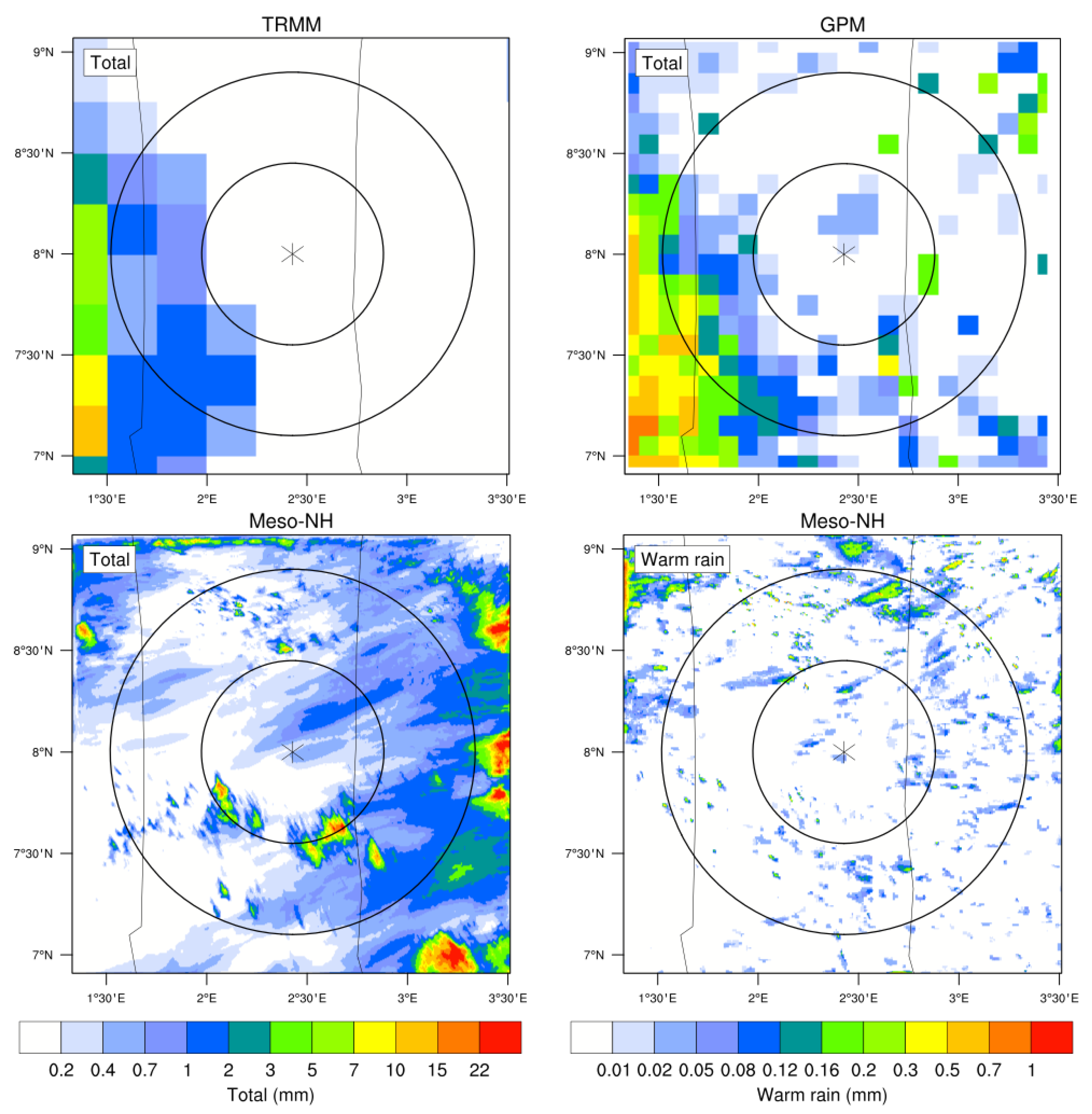
We inspect how total rainfall is spatially distributed in the simulation, and compare that with two gridded satellite observations, the TRMM 3B42V7 product (3 h, 0.25${}^{\circ }$) and the GPM IMERGV06B product (30 min, 0.1${}^{\circ }$). Figure 6 shows maps of the total accumulated rainfall from 03:00 to 09:00 UTC for the three datasets, as well as warm rain for the simulation.

The analysis of rainfall at ground is done from 03:00 to 09:00 UTC (instead of 08:00 UTC) due to the 3-hourly temporal resolution of the TRMM product. Notice that although the colorbars are the same in Figure 6, their values differ between the maps for total and the map for warm rain. Both satellite products retrieve rainfall with values of 5 mm or more to the west of the domain. It corresponds to the signature of a MCS over western Benin and Togo. While TRMM only shows precipitation from the MCS, GPM retrieves rainfall with values up to 7 mm over the eastern half of Benin and over Nigeria. Inside the X-band radar range, the small patterns oriented in the southwest-northeast direction suggest they correspond to warm-rain features or isolated storms. Moreover, GPM retrieves 0.2–0.4 mm over the gridpoint adjacent to Savè, although it is a lower value than the 1.6 mm measured at the supersite. The discrepancy between TRMM and GPM points out the challenge that satellites currently face to capture warm rain and shows the potential of GPM with respect to TRMM. In the simulation, rainfall over Togo is missed, because the MCS is simulated further west (in the 1-km resolution simulation) and is smaller than observed (not shown). Over the eastern boundaries of the domain, large precipitating systems are simulated, in partial agreement with GPM. Inside the radar range, rainfall greater than 5 mm is unevenly distributed and mainly corresponds to deep convection. Smaller precipitation features of less than 3 mm may correspond to shallow clouds. Rainfall below 3 mm mimics the southwest-northeast orientation seen in GPM. The simulated warm rain is sparsely scattered. It sometimes appears as strips or structures with the GPM-like orientation.

The total rainfall observed by TRMM and GPM is 0.8 and 1.5 mm, respectively, and it is 1.0 mm for the simulation. This is encouraging given the short frame of the reporting period. We also estimated the contribution of warm rain to total rainfall and to the area covered by rain. These contributions cannot be calculated for satellite products due to the lack of observed vertical distribution of precipitating hydrometeors. For the simulation, the contribution of warm rain to total rainfall is 1.2%. Although this contribution is only calculated for a 6-h period (from 03:00 to 09:00 UTC), its order of magnitude compares well with the 1.35% warm rain recorded at Savè during the whole campaign and the climatological value of 2% obtained by [9]. While warm rain contributes little to rainfall, its contribution to the area covered by rain is much larger: almost one fourth (24.4%) of the area covered by rainfall is covered by warm rain.

4. Characteristics of the Warm-Rain Cells

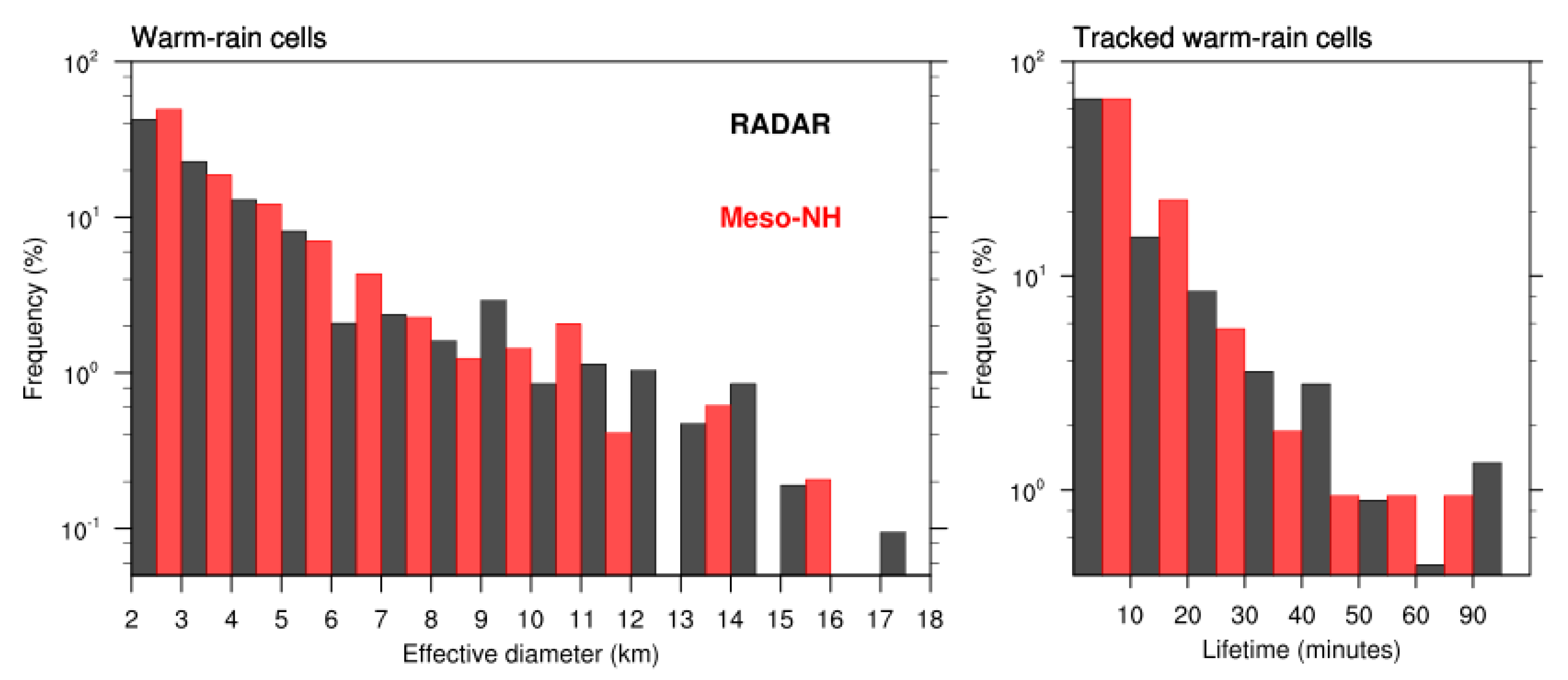
The relative distributions of the effective diameter of the warm-rain cells and the lifetime of the tracked warm-rain cells are represented in Figure 7 for the X-band radar and the simulation. The lifetime distribution is shown for a 20% geographical overlap. In both datasets, the number of warm-rain cells decreases with increasing diameter. The total number of 1057 observed warm-rain cells is in agreement with the number detected by the X-band radar, which is in average 20 per 5 min scan. Only 485 warm-rain cells are simulated. Although the simulated warm-rain cell population counts about half the observed number, the relative distribution is well captured. The large majority of warm-rain cells have diameters below 5 km, approximately 78% in the observations and 81% in the simulation. 17% and 16% warm-rain cells in the observations and the simulation, respectively, have diameters comprised between 5 and 10 km. The remaining 5% and 3% correspond to cells with diameters larger than 10 km. The largest diameters are 17.3 km in the radar and 15.9 km in the simulation.

The number (225) of observed tracks (warm-rain cells detected at least at two successive steps) approximately doubles the number of the ones that are simulated (107). This is due to an underestimation of the number of simulated warm-rain cells during the nighttime, as will be shown later. Among the total number of tracks, 67% last up to 10 min for both the radar and the model and 31% and 32% of the observed and simulated tracks, respectively, last between 15 min and 1 h. Lifetime rarely exceeds 1 h. The distribution was calculated using a 20% overlap value. Values from 5 to 40% with an increase of 5% were tested and the sensitivity of the distribution to the threshold has been found to be generally low. Overlapping thresholds in the range from 5 to 30% have little to no impact on the duration of the tracks, with roughly 2/3 of the tracked warm-rain cells that exist for 5 to 10 min, 1/3 that last between 15 and 60 min and 1 to 3% that last longer. Adopting a threshold of 35% or more is, however, more restrictive, such that the frequency of 5–10 min duration reaches about 3/4 of the tracked warm-rain cells. This results in a diminution of the mean lifetime. This is the first time that the lifetime of warm-rain cells is quantified, and has been possible because of their individual identification.

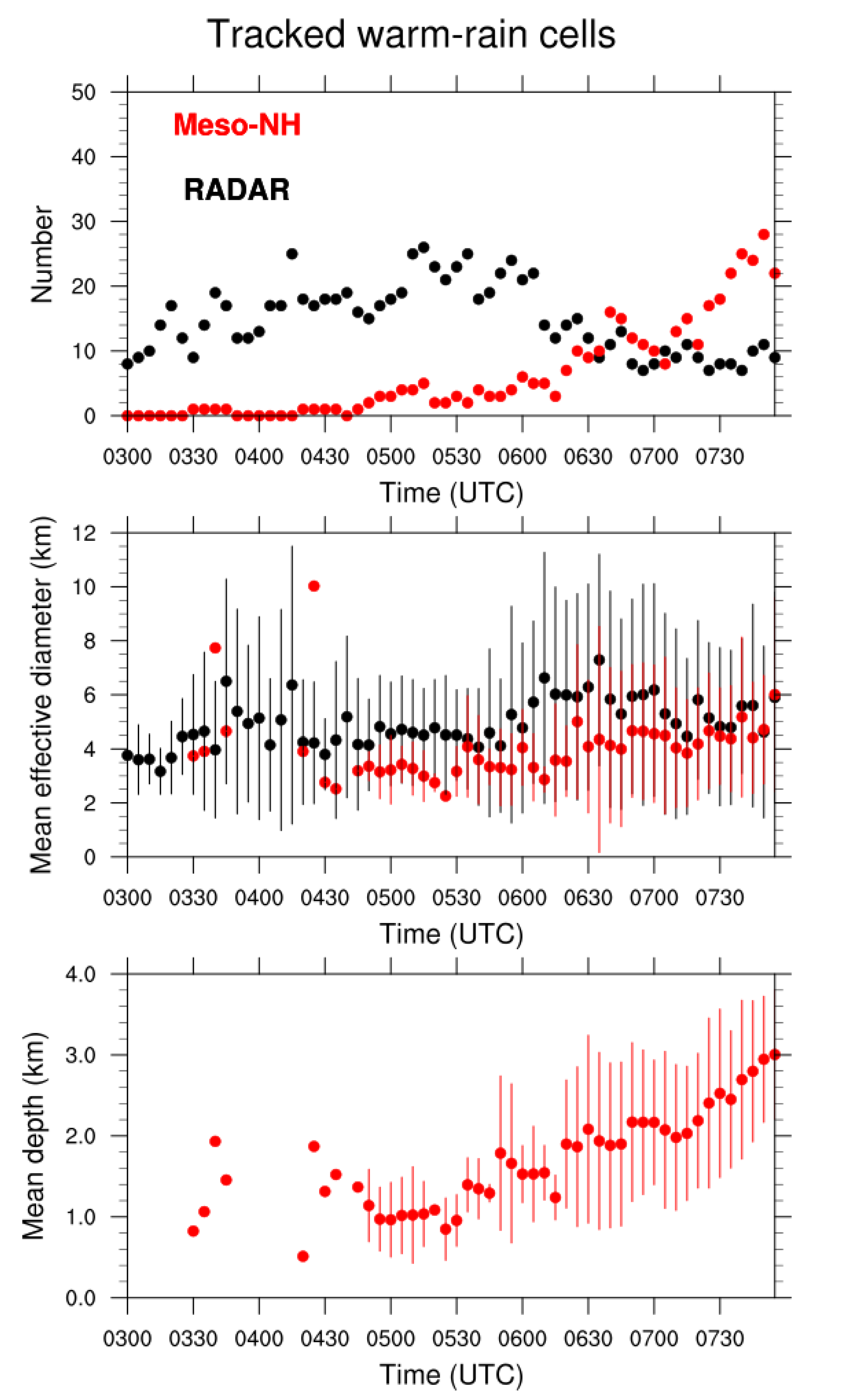
The time evolution of the number and effective diameter of the tracked warm-rain cells is presented in Figure 8 for the radar and the simulation. The simulated depth (calculated as the difference between the top and the base) is also shown. The number of observed tracks increases from around 10 detections per 5 min scan at 03:00 UTC to 20–30 detections at 06:00 UTC. Later on, their number diminishes. Very few warm-rain cells are simulated during the nighttime, then the population grows fast from about 5 detections at 06:00 UTC, which corresponds to sunrise in Savè [17], to more than 20 towards the end of the analysis period. The triggering of warm-rain clouds is enhanced due to the daytime increase of the surface fluxes and the development of the boundary layer. Overall, the mean effective diameter slightly increases for both the observed and simulated tracks. The simulated warm-rain cells also become deeper with time as the surface fluxes increase, from 1-km depth at 05:00 UTC to 3-km depth by 08:00 UTC. In average, the observed tracked warm-rain cells have their tops at 2315 m high. In the LES, the average base and top are 1709 and 3876 m, respectively.

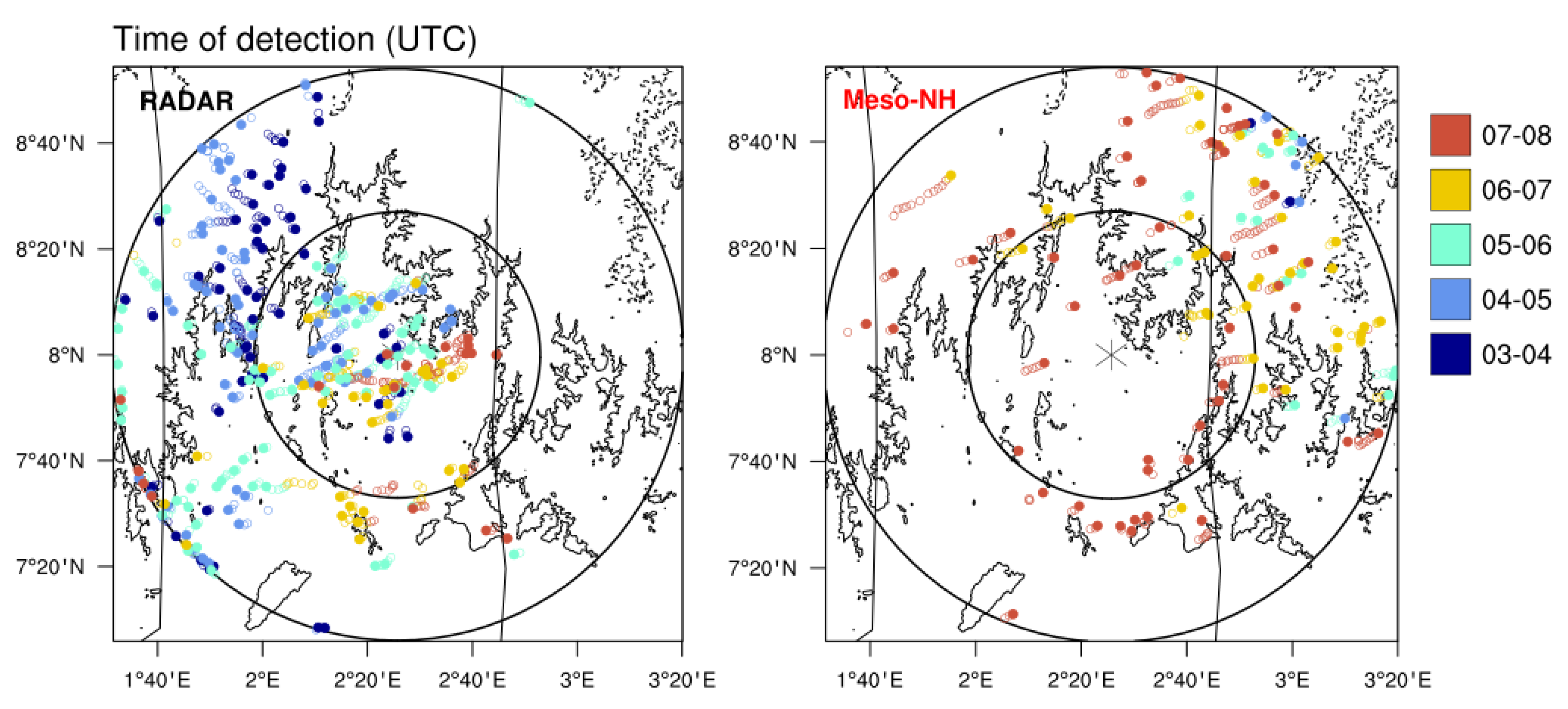
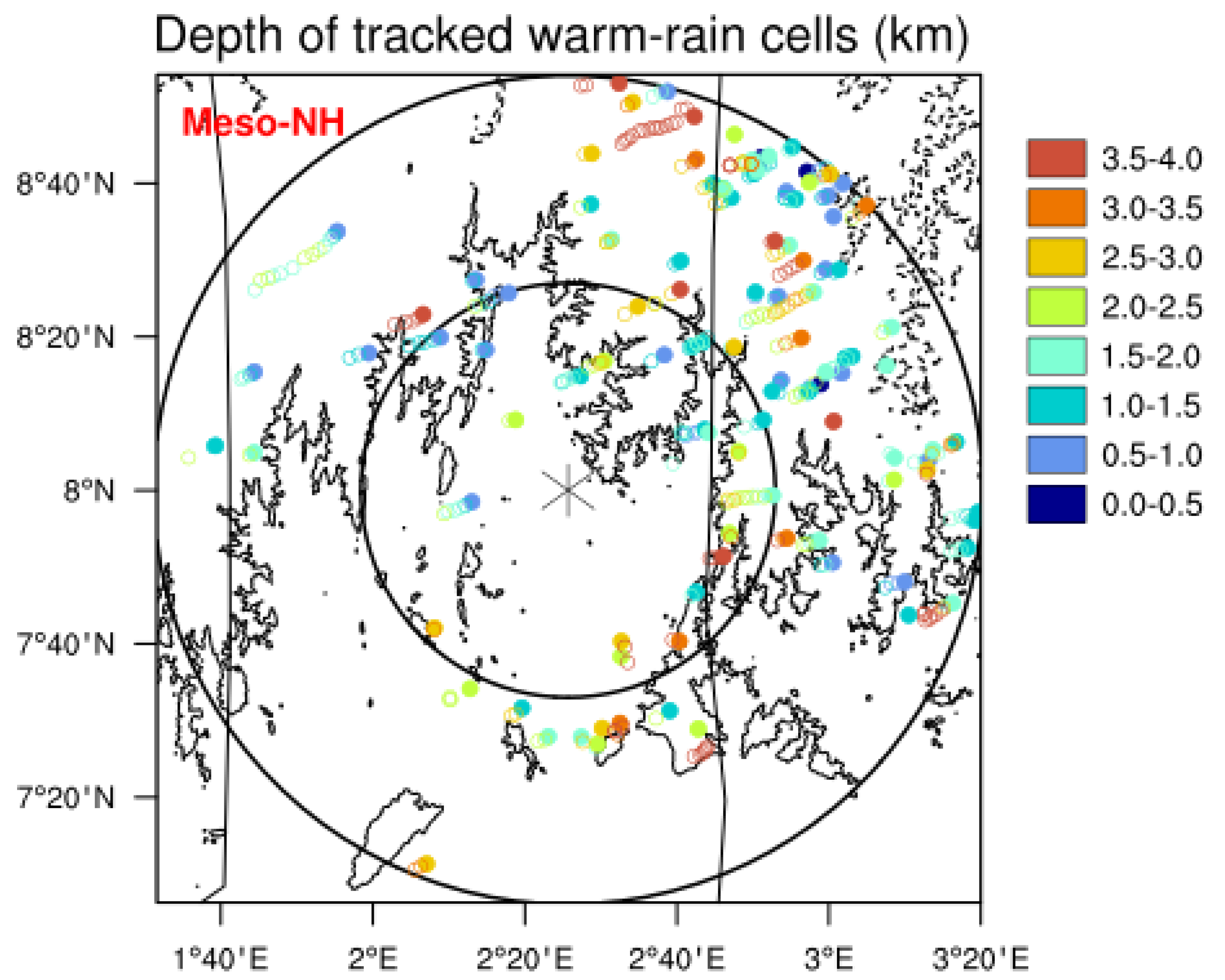
Figure 9 and Figure 10 show the spatial distribution of the tracked warm-rain cells; the colors display the hour of detection for the radar and the LES in Figure 9 and the simulated depth of the warm-rain cells in Figure 10. The solid dots depict the first detection of each track, the empty dots depict the consequent detections. The majority of the observed nighttime warm-rain cells (from 03:00 to 06:00 UTC) are located inside the outer 50-km radar range, in the western half of the domain, whereas the daytime ones (fewer in number) are mainly in the inner 50-km range, some of them lying slightly south. The simulated tracked warm-rain cells, less numerous, are generally distributed over the northeastern quadrant, as seen from Figure 8. The vast majority appear after 06:00 UTC. The observed nighttime warm-rain cells present higher tops. An analysis of MSG-derived brightness temperature indicates that during the nighttime, the observed warm-rain cells tend to develop near cold cloud tops above the 0${}^{\circ }$ C altitude (not shown), and probably correspond to transient stages of deep convection. Some of them are located in the vicinity of the MCS. In the simulation, the vertical extension of the clouds covers the full range of depths.

For the radar, the trajectories of the warm-rain cells show two predominant directions, probably corresponding to two different wind regimes. The nighttime warm-rain cells in the northwestern part of the outer 50-km range, where they generally have higher tops, present a southeasterly propagation. Another group of nighttime and daytime warm-rain cells show preferentially a southwesterly propagation. Finally, a few tracks are rather stationary and appear near orographic features. In the simulation, they mainly show a northeasterly propagation. The long tracks seem to span over longer distances than for the radar. This is possible if they are found within a larger wind speed regime.

In summary, almost every tracked warm-rain cell (98%) lasts 60 min at most, according to the X-band radar. The tracked warm-rain cells present mean effective diameter and top height of 4.9 and 2.3 km, respectively. The LES captures remarkably well the size and lifetime relative distributions. However, the total number of simulated warm-rain cells is underestimated, mainly during the nighttime. They also present tops too high by ∼1.6 km in average. This can affect the amount of warm rain by changing the height in the atmosphere and the path within the cloud in which the collision-coalescence processes occur. The LES has trouble representing the spatial distribution of warm-rain cells partly because of the absence of the MCS, which might also explain the lack of nocturnal warm-rain cells. The LES compares better with the observations during the day, but the main drawback is the simulated southwestward propagation compared to the observed northeastward motion.

5. Vertical Structure of the Atmosphere and the Warm-Rain Cells

To better understand the main processes driving the development of warm-rain-producing clouds in the observation and the LES, the vertical structure of the atmosphere at Savè on 24 July 2016 is now examined as well as the vertical properties of the simulated tracked warm-rain cells.

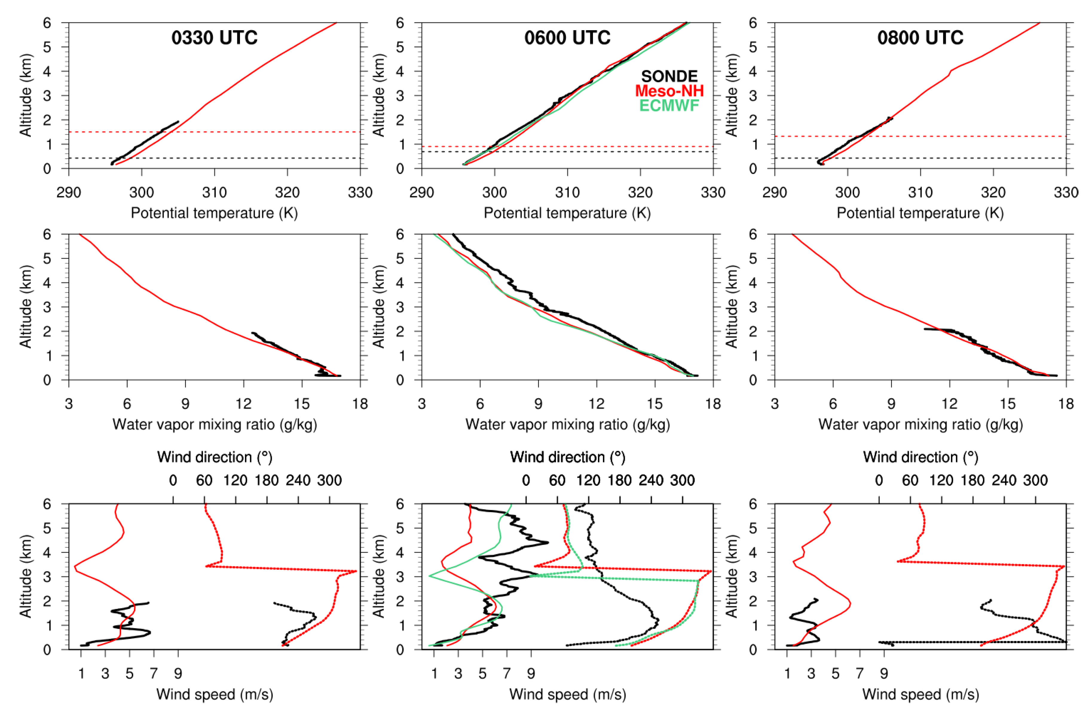
The vertical profiles of potential temperature, water vapor mixing ratio and wind speed and direction from the radiosoundings at Savè and from the simulation are shown in Figure 11 at 03:30, 06:00 and 08:00 UTC. Profiles of the same variables are also displayed for the ECMWF operational analysis at 06:00 UTC (i.e., when available). The observed potential temperature shows the static stability of the atmosphere at 03:30 and 06:00 UTC. At 08:00 UTC, the daytime development of the boundary layer causes a neutral stratification in the first 200 m. The observed water vapor mixing ratio at the surface takes values between 16 and 17 g kg${}^{-1}$, then it decreases with altitude. These near-surface values of moisture content lie within typical values at the Savè site [17]. The profiles at 03:30 and 06:00 UTC are moister than at 08:00 UTC in the lowest 2 km, probably due to daytime mixing. At 03:30 UTC, the observed wind speed shows a maximum of more than 6 m s${}^{-1}$ at around 700 m altitude, with a southwesterly direction. This is the signature of the nocturnal low-level jet, with an intensity and core height typical of Savè [34,35]. At 06:00 UTC, the low-level jet has disappeared and southwesterlies of 3 to 7 m s${}^{-1}$ are observed up to around 2 km, corresponding to the monsoon flow. The mean depth and wind speed of the monsoon layer at Savè are 1.9 km and 6 m s${}^{-1}$ [17]. At 08:00 UTC, the wind speed shows two maxima of 3–4 m s${}^{-1}$.

The LES presents a warm bias, of 1 to 2 K, between the surface and around 2 km with respect to the observations. This bias is the largest at 03:30 and then decreases. The profiles of water vapor mixing ratio at 03:30 and 06:00 UTC capture well the values from the soundings up to 1.5 km. Then, they depart from the observations and become drier. At 08:00 UTC, the simulation overall captures the observed values of water vapor mixing ratio. The nocturnal low-level jet at 03:30 UTC is simulated, but with a wind speed of 4 m s${}^{-1}$ lower than observed. The monsoon flow is reproduced by the simulation with a correct wind direction up to approximately 1.5-km high. Then, the simulated wind exhibits a wrong northwesterly direction and does not capture the observed veering of the wind. Above 3.5-km altitude the simulated wind presents a northeasterly direction, whereas it is southeasterly according to the observations. The wind in the operational analysis of the ECMWF also turns wrongly at the same altitude, indicating that the wind bias in the simulation is largely influenced by the synoptic-scale winds imposed at the initial and boundary conditions. At 08:00 UTC, the simulation misses the wind direction in the first 500 m, probably because of some local event absent in the simulation. Above, the same wind pattern from 03:30 and 06:00 UTC prevails due to the wrong large-scale winds.

Overall, the stable atmosphere at Savè is well captured by the LES. The latter shows, however, a warm bias below 2 km and a dry bias above. The height of the lifting condensation level ($z_{LCL}$) for an air parcel departing from the surface is also represented in Figure 11. It is computed using Equation (24) from [36]:

$$z_{LCL}\approx z_{sfc}+\left(20+\frac{T}{5}\right)(100-RH),$$

(1)

where $z_{LCL}$ and $z_{sfc}$ are given in m, T is in ${}^{\circ }$C and $RH$ in %. $z_{LCL}$ has been calculated for an air parcel departing from the surface and is representative of the lower atmosphere. For the three soundings, $z_{LCL}$ is larger for the LES compared with the soundings (∼730 m average difference). This is due to the warm bias up to 2-km altitude, that partly explains why the simulated warm-rain clouds develop higher in the atmosphere.

Despite the punctual character of these wind profiles, the incorrect wind direction above ∼1.5-km altitude is persistent. Thus, the simulated warm-rain cells, with mean tops at 3.9 km, are wrongly advected from the northeast, as shown from Figure 9. However, in the observations they generally lie below, within the monsoon flow, and exhibit a southwesterly propagation. The observed and simulated mean top height of the warm-rain cells (2.3 and 3.9 km, respectively) correspond to the height where the wind shear is the largest (veering). The observed warm-rain cells develop throughout the depth of the moist monsoon flow whereas in the simulation they grow in the dry northeasterly wind sector. The latter is, at the same time, responsible for the simulated dry bias as air is advected from the drier Sahelian middle atmosphere. This notable discrepancy on the wind direction comes from the initial conditions as these soundings launched during 24 July 2016 were not assimilated in the Integrated Forecasting System of the ECMWF. Furthermore, the denial experiment carried by [37] for the DACCIWA campaign shows that, in the absence of radiosonde assimilation, the main biases in the ECMWF forecasts occurred in the lower atmosphere, especially on wind and temperature during the night and early morning.

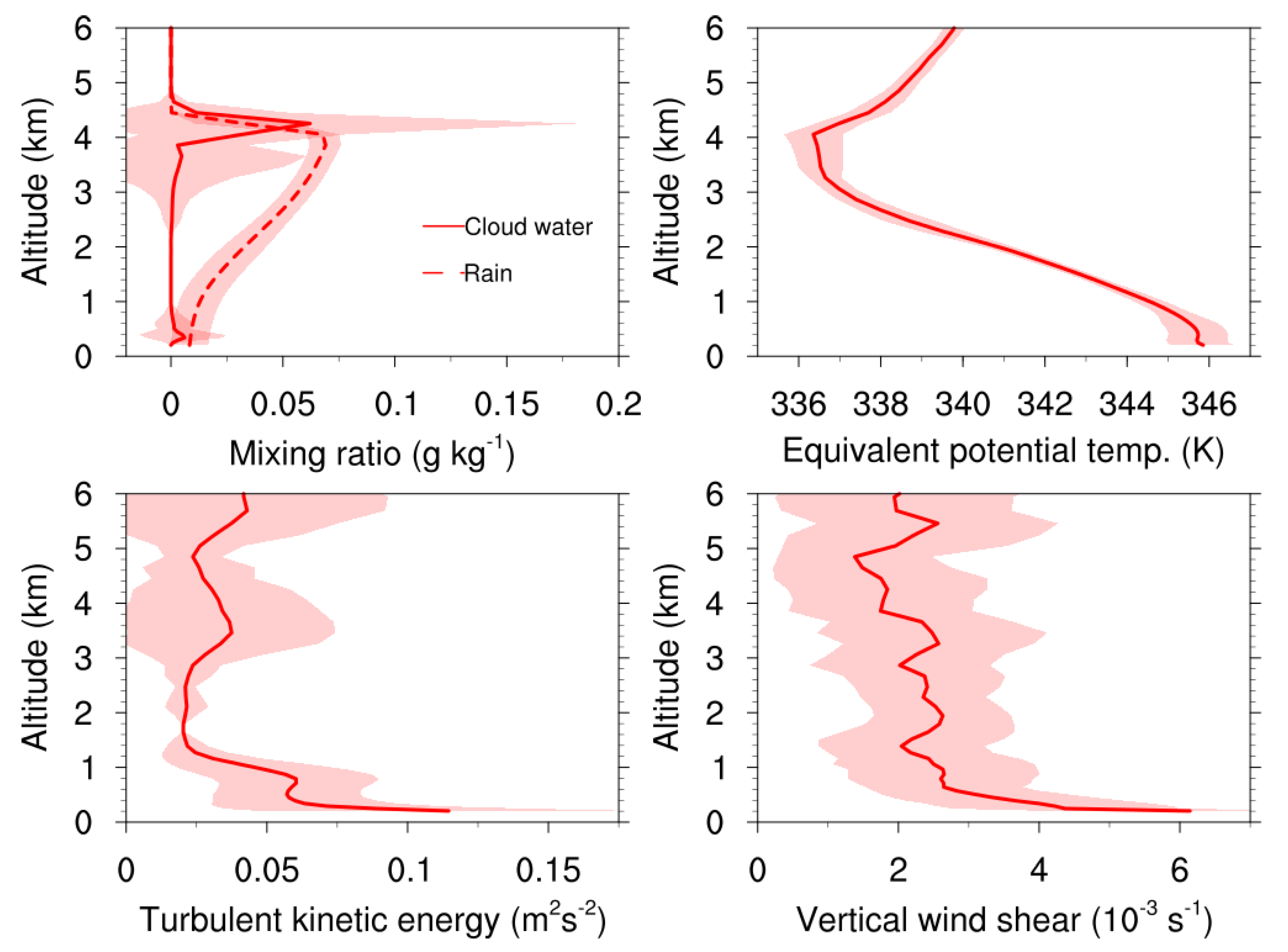
We further investigate the properties inside the simulated warm-rain clouds. The mean vertical profiles (and variability) of cloud and rain water, equivalent potential temperature (${\theta }_e$), turbulence kinetic energy (TKE) and vertical wind shear are shown in Figure 12. The individual profiles are calculated at the center of mass of the tracked warm-rain cells, but only with depths lower than 2 km (which have mean base and top at 2.5 and 3.9 km). The reason for using this reduced sample is that the warm-rain clouds observed by the cloud radar at Savè show tops around 2-km height (Figure 5).

The mean rain mixing ratio is positive at the surface, meaning that, in average, rainfall reaches the ground, although the warm-rain base (defined at 20 dBZ) is higher. It then increases until it reaches its maximum value of 0.07 g kg${}^{-1}$ at 4-km altitude, and then decreases sharply and vanishes at 4.5 km. Note that the actual top of the warm-rain clouds can lie above 4 km. Indeed, there is a peak in cloud water content between 4 and 4.5-km high. Below, the cloud water mixing ratio diminishes drastically whereas rain is present, probably due to too fast autoconversion and accretion of cloud droplets. The profile of ${\theta }_e$ shows a maximum value of 346 K at the surface, and then decreases down to a value around 336 K at 4-km high. This minimum value of ${\theta }_e$ at 4-km high explains the too high tops found in the simulation with respect to the observations. The simulated clouds grew through the depth of the unstable layer. The largest values of TKE and wind shear are found in the boundary layer, with a peak at around 800 m. TKE is minimum between ∼1.2 and 2.4 km, above the boundary layer and below the warm-rain cell base. Then, larger values of TKE are found up to 4.5 km, due to in-cloud eddies and turbulence. TKE shows a peak of 0.035 m${}^2$ s${}^{-2}$ at around 3.5 km. Also at that height, a local maximum of 2.5 × 10${}^{-3}$ s${}^{-1}$ is reported for the vertical wind shear. It is found within a 1-km thick layer just below the warm-rain cells top. This indicates, in agreement with Figure 11, that the warm-rain clouds are capped by a high-sheared layer.

6. Conclusions

Warm rain around Savè, Benin, in southern West Africa (SWA) is explored during the case of 24 July 2016, as part of the DACCIWA project. The event yielded 1.6 mm warm rain in Savè, which was one of the three supersites of the field campaign during summer 2016. This amount represents roughly half of the warm rain recorded at the supersite. Overall, total warm rain contributed to 1.35% of total rainfall during the two-month campaign. Several instruments deployed in Savè served to document this warm-rain episode, particularly the X-band rain radar deployed by the KIT. This radar can identify warm-rain features because it delineates the volume of precipitating hydrometeors and determines the top heights, allowing the characterization of the warm-rain cells. A 200-m grid spacing LES run with the Meso-NH model is also used to investigate warm rain, its contribution and its drivers.

The analysis of warm rain is performed from 03:00 to 08:00 UTC, when it was reported at Savè. The detection of warm-rain cells is based on reflectivity retrieved by the X-band radar and simulated by the model at high-temporal frequency. We apply a clustering algorithm to masked reflectivities (>20 dBZ) and determine the vertical development of each cluster or rain cell. If the clusters have tops below 4 km and diameters larger than 2 km they are defined as warm-rain cells. These are also tracked in time, which allows the quantification of their lifetime.

The 5-h analysis of warm-rain cells shows that 78% of the 1057 observed ones have diameters between 2 and 5 km, and only 5% have diameters larger than 10 km. Among the 225 warm-rain cells that were tracked at least twice, approximately two-thirds exist for 5 or 10 min, and approximately one-third exist for 15 min to 1 h. Only a residual percentage of tracks last longer than 1 h. Although the number of both instantaneous and tracked warm-rain cells is roughly half in the simulation, the model reasonably captures the size and lifetime relative frequency distributions.

The observed tracked warm-rain cells lie mainly in the western half of the radar domain. While most of the nighttime warm-rain cells (detected before 06:00 UTC) lie in the outer 50-km radar range and have higher tops, the daytime cells (after 06:00 UTC) are mostly found in the inner 50-km radar range and are shallower. During the night, warm rain is mainly linked to evolving phases of deep convection. During the day, it comes from pop-corn-like shallow convection. Most of the simulated tracked warm-rain cells are located in the eastern half of the domain. They trigger only after sunrise and extend 1.6 km higher in the atmosphere. The observed (simulated) top is 2.3 km (3.9 km), and the simulated base is 1.7 km. While in the observations the predominant direction of propagation is southwesterly, with most of the tracked warm-rain cells embedded in the 2-km thick monsoon flow, the simulated cells exhibit a northeasterly propagation. In other words, the model is able to produce warm rain during this case. It also reproduces, in a satisfactory manner, the size and lifetime of warm-rain cells, but has trouble simulating their spatial distribution, direction of propagation and vertical development.

The main drawbacks in the propagation and vertical extension in the model come from biases in the meteorological fields provided by the initial and boundary conditions. On the one hand, a 1–2 K warm bias in the two first kilometers with respect to the radiosounde measurements at Savè renders the simulated lower atmosphere more unstable and favors the vertical growth of the warm-rain clouds. On the other hand, the simulated wind direction above approximately 1.5-km altitude, where the simulated warm-rain cells propagate, is wrong. This failure is attributed to the wrong large-scale forcing from the ECMWF operational analysis.

The amount of warm rain is further computed in the simulation from the ground rainfall covered by the warm-rain cells. It is found that 1.2% of total rainfall is due to warm rain. Interestingly, the contribution to the area covered by warm rain is much larger (24.4%). This means that warm rain has the potential to distribute rainfall over large areas and suggests that warm rain might be of high importance during the drier periods that SWA experiences during the monsoon season [11]. Although the simulated 1.2% contribution to warm rain is only calculated for a 6-h period, it compares well in order of magnitude with the 1.35% contribution in Savè during the DACCIWA campaign, and with the 2% estimation by [9] in its climatology over the coastal regions of SWA.

This is the first time that warm-rain amounts are quantified from a LES over SWA. The results shown here remain, however, limited, as only one single warm-rain event was studied. Other cases should be investigated. Currently unknown tendencies and seasonal and interannual variability of warm rain in SWA could be addressed by applying the reliable yet inexpensive warm-rain cell detection method used here to longer simulations or radar databases. This study reflects that uncertainties are intrinsic to any data source, which contributes to the known issue of model-observation comparison. The comparison done here indicates that, while a 200-m grid permits shallow convection, proper large-scale conditions remain fundamental to entirely reproduce the warm-rain properties in limited-area models. Further observational efforts are needed to improve today’s operational analysis, probably in the form of continuous observations rather than intensive field operations.

This paper demonstrates the challenge that high-resolution simulations face to capture fine-scale processes leading to warm rain formation in southern West Africa. Because the large-scale forcing was not reliable enough, the representation of the physical processes in the model has not been tested here. Addressing the sensitivity of warm rain to warm-rain microphysics, in particular to the critical cloud water content beyond which autoconversion is initiated, could be a pathway for future research.

7. Data Availability

The DACCIWA data from the Savè supersite are available on the SEDOO database (http://baobab.sedoo.fr/DACCIWA/). The Meso-NH output data are available from I.R.M. upon request.