Article

Development of Multiple Linear Regression for Particulate Matter (PM10) Forecasting during Episodic Transboundary Haze Event in Malaysia

by
Samsuri Abdullah
1,*,
Nur Nazmi Liyana Mohd Napi
1,
Ali Najah Ahmed
2,3,
Wan Nurdiyana Wan Mansor
1,
Amalina Abu Mansor
4,
Marzuki Ismail
4,5,
Ahmad Makmom Abdullah
6 and
Zamzam Tuah Ahmad Ramly
6,7
1
Air Quality and Environment Research Group, Faculty of Ocean Engineering Technology and Informatics, University Malaysia Terengganu, Kuala Nerus 21030, Malaysia
2
Faculty of Engineering, University Tenaga Nasional, Bangi 43650, Malaysia
3
Institute of Engineering Infrastructures, University Tenaga Nasional, Bangi 43650, Malaysia
4
Faculty of Science and Marine Environment, University Malaysia Terengganu, Kuala Nerus 21030, Malaysia
5
Institute of Tropical Biodiversity and Sustainable Development, University Malaysia Terengganu, Kuala Nerus 21030, Malaysia
6
Faculty of Environmental Studies, University Putra Malaysia, Serdang 43400, Malaysia
7
Enviro Excel Tech Sdn Bhd., A-G-09, Univ 360 Places, Seri Kembangan 43300, Malaysia
*
Author to whom correspondence should be addressed.
Atmosphere 2020, 11(3), 289; https://doi.org/10.3390/atmos11030289
Submission received: 5 February 2020 / Revised: 13 March 2020 / Accepted: 13 March 2020 / Published: 16 March 2020
(This article belongs to the Section Air Quality)

Abstract

:
Malaysia has been facing transboundary haze events every year in which the air contains particulate matter, particularly PM10, which affects human health and the environment. Therefore, it is crucial to develop a PM10 forecasting model for early information and warning alerts to the responsible parties in order for them to mitigate and plan precautionary measures during such events. Therefore, this study aimed to develop and compare the best-fitted model for PM10 prediction from the first hour until the next three hours during transboundary haze events. The air pollution data acquired from the Malaysian Department of Environment spanned from the years 2005 until 2014 (excluding years 2007–2009), which included particulate matter (PM10), ozone (O3), nitrogen oxide (NO), nitrogen dioxide (NO), carbon monoxide (CO), sulfur dioxide (SO2), wind speed (WS), ambient temperature (T), and relative humidity (RH) on an hourly basis. Three different stepwise Multiple Linear Regression (MLR) models for predicting the PM10 concentration were then developed based on three different prediction hours, namely t+1, t+2, and t+3. The PM10, t+1 model was the best MLR model to predict PM10 during transboundary haze events compared to PM10,.t+2 and PM10,t+3 models, having the lowest percentage of total error (28%) and the highest accuracy of 46%. A better prediction and explanation of PM10 concentration will help the authorities in getting early information for preserving the air quality, especially during transboundary haze episodes.

1. Introduction

Haze pollution has become an international issue as it affects the local, regional, and global air quality, especially in Southeast Asian (SEA) countries, including Malaysia, Singapore, Indonesia, Brunei Darussalam, and Southern Thailand [1,2,3]. Haze occurs annually due to periodic biomass burning, such as forest fires, peatland combustion, and agricultural burning in Sumatra and Kalimantan, Indonesia. The influence of unpredictable monsoon rain and El-Nino phenomenon both worsens the transboundary haze due to the prolonged and drier weather conditions, especially during the southwest monsoon season [3,4,5,6,7,8]. These conditions increase the severity of air quality due to it containing a noxious mix of air pollutants, such as particulate matter and noxious gases, which are collectively influenced by meteorological factors like ambient temperature, relative humidity, and wind speed [9,10]. Malaysia has been facing this awful phenomenon for almost over a decade, which started in the 1980s up until recent years [5,11,12]. Haze is detected when the atmosphere contains a higher concentration of particulate matter suspended in the air, which either can or cannot be observed by the naked eye when the relative humidity is lower than 80% and the visibility is reduced to 10 km [5,13,14,15]. Daily particulate matter with 10 micro aerodynamic diameters (PM10) exceeding 150 µg/m3 for 24 h of permissible limit is thus notified as haze, which is set under the new Malaysian Ambient Air Quality Standard (NAAQS) by the Department of Environment, Malaysia.
Biomass peat soil combustion generally emits the particulate matter and gaseous pollutants, as well as their components such as anions, cations, heavy metals, and levoglucosan [16,17,18,19]. Carbon monoxide (CO) is higher during haze events compared to other gases due to the characteristics of peatland areas, which are rich in carbon materials. It is emitted through the incomplete combustion process of carbonic materials in the presence of a minimum amount of oxygen. Meanwhile, PM10 contains a high concentration of NO3 anion produced through bacterial nitrification and oxidation process during combustion, while SO42− cation is also found in a high amount due to pesticide application in the peat soil, thereby slowing down the accumulation of sulfur [18]. Those ions originate from sulfurous and nitrogenous materials as they will be converted to such particles via gas-to-particle conversion. Similarly, heavy metals from the peatland soil are converted to particulate matter by the combustion process in which the characteristics of heavy metals will be contained in the ash suspended in the air [17,18]. The isomeric anhydrous sugar levoglucosan is found in the fine particulate matter during transboundary haze as it is known as a specific and general indicator of biomass emission composition directly emitted into the atmosphere. It is yielded by some anthropogenic activities such as wood burning and biogenic activities, as well as the by-product of secondary photochemical oxidation of organic precursors [16].
Every time the haze phenomenon hits the country, it will inhibit the economic and social developments; the country will need to bear higher medical costs due to drastically increased outpatient and inpatient numbers. This was estimated to be approximately MYR273,000 (USD91,000) based on the data from 2005 until 2009 for 14 haze-related illnesses suffered by the public [5,20]. Moreover, when the haze event worsens and it is declared unsafe, hundreds of schools in the affected areas are closed, communication becomes limited, and people will need to reduce outdoor activities in order to minimize their exposure to it [21,22]. Therefore, the tourism sector is also affected during these events in terms of the economy, human perception, and the environment. Similarly, huge losses occur when the atmospheric visibility decreases; many flights are cancelled due to unsafe conditions to fly, which decreases the number of tourism activities. Furthermore, the number of extinct plants, animals, and biodiversity will increase due to extreme environmental events, while the circumstances can also change tourism moods due to unsatisfactory environmental conditions and lead to a refusal to revisit [5,10,21,22].
Toxic particles in haze harm human health either in cumulative or acute effects like respiratory mortality, cardiovascular illness, and lung cancer to all groups of people, such as adults and children [9,20]. The small particulate size contained in haze can easily penetrate the lung; at worst, it also goes into the bloodstream [22]. Based on the previous study by [4], long-term exposure to air pollution causes an increase in neurological diseases such as cerebrovascular disease and stroke, along with headache and migraine symptoms. Skin is one of the organs that are directly in contact with air pollution, especially during transboundary haze events. The small particulate matter enters through the skin via the pores, causing allergic symptoms and skin damage, such as skin irritation and inflammation, damaged skin barrier function, increased rate of ageing, and influences on the composition of skin lipid [23,24,25]. In the worst-case scenario, long-term exposure to air pollution causes an increase in the degree of skin sensitivity and causes skin defect, as well as atopic dermatitis [23].
During transboundary haze events, particulate matter, especially the harmful PM10 pollutant, needs to be predicted for determining and understanding its dispersion behavior in the atmosphere. This can provide information to the concerned people and their awareness to reduce outdoor activities at the affected areas [26]. The Multiple Linear Regression (MLR) model is globally and widely used over many years as a method for air pollution forecasting, which can help to attempt the uncertainty of the future simply by relying on past and current data for decision-making [27,28,29]. The fundamental basis of this model represents the relationship between the dependent variable and several independent variables, such as meteorological factors and gaseous pollutants, by uncomplicated computation and easy implementation [30,31]. Previous studies in Malaysia have developed the MLR model to predict PM10 concentration, specifically in the East Coast Peninsular Malaysia, based on different site classifications of rural, suburban, urban, and industrial areas and during different types of monsoon to determine its variation during non-haze periods [27,32,33]. Moreover, [34] used the MLR model for PM10 forecasting during haze events that hit Malaysia based on the data from the affected Air Quality Monitoring Station (AQMS). Therefore, this study aims to determine the annual variation of PM10 concentration during transboundary haze events and develop the models to investigate the relationship linking PM10 with meteorological factors and gaseous pollutants, which are contributing to the high PM10 concentration. PM10 is used in this study as the dependent parameter for the prediction purposes as the Malaysian Department of Environment had started to monitor the PM2.5 concentration in 2018. However, the episodic haze events need a long period of dataset, which is the main reason to use PM10 in this study. These research findings will help the responsible parties in providing early warning information to come out alongside mitigation and precautionary plans to improve the air quality during haze events, as well as protect the public health.

2. Materials and Methods

2.1. Study Area and Data Collection

Malaysia faces a periodic transboundary haze event due to the large-scale biomass combustion in Sumatra, Indonesia, which happens almost throughout the year and affects the Peninsular Malaysia, Sabah, and Sarawak regions [6]. The haze event usually occurs during the months of January to February and June to August every year [22]. Figure 1 and Table 1 show the location of the affected Air Quality Monitoring Station (AQMS) where the air pollution data are obtained. Data were obtained from the years 2005 until 2014 with the exclusion of years 2007 to 2009 from the Air Quality Division, Department of Environment (DOE), Ministry of Natural Resources and Environment of Malaysia. They were tabulated and arranged based on the chronological timeline of haze episodes in Malaysia [14] in Microsoft Excel Spreadsheet® 2016 and analyzed using Statistical Packages for Social Sciences (SPSS®) version 25. The parameters used in this study were particulate matter with an aerodynamic diameter less than 10 µm (PM10, µg/m3), ambient temperature (T, °C), relative humidity (RH, %), wind speed (WS, km/hr), ground-level ozone (O3, ppm), nitrogen oxide (NO, ppm), nitrogen dioxide (NO2, ppm), carbon monoxide (CO, ppm), and sulphur dioxide (SO2, ppm) to gain a better picture of PM10 variability during transboundary haze. The relationship between these parameters was examined using bivariate correlation analysis in which the PM10 concentration was measured using the β-ray attenuation mass monitor (BAM-1020) as manufactured by Met One Instruments Inc. [27]. Meanwhile, the meteorological parameters were measured using Met One 062 sensor for ambient temperature, Met One 083D sensor for relative humidity, and Met One 010C sensor for wind speed [35]. The Teledyne API Model 400/400E instrument hourly through UV absorption (Beer-Lambert) method with a 0.4ppb detection limit and 0.5% of precision level and Model 200A NO/NO2/NOx analyzer, which applies chemiluminescence detection principles was used to detect O3, NO2, and NO concentrations in ambient air, respectively [36,37]. The SO2 and CO concentrations were monitored and measured by the Teledyne API Model 100A/100E and Teledyne API Model 300/300E, with the lowest detection level of SO4 at 0.04 ppb by the UV fluorescence method. Meanwhile, the CO level was measured with 0.5% precision and the lowest detection was found at 0.04 ppm by the non-dispersive and infrared absorption (Beer-Lambert) method [37]. Therefore, all instruments were set to have daily calibration using zero air and standard gas concentration to guarantee the quality control and assurance of data monitoring and validation processes, which were revised before they were transferred to the DOE [38]. Missing data might occur due to equipment malfunction and the calibration program, which were thus removed to reduce the bias in the prediction and conservative results [39].

2.2. Multiple Linear Regression

Stepwise Multiple Linear Regression (MLR) statistical models were developed in this study with a 95% confidence interval and the dataset was separated according to 7:3 ratios for model development and validation, respectively [40,41]. Based on the data tabulated in the Microsoft Excel Spreadsheet® 2016, 70% of the earlier data in this spreadsheet were used for model development, while the remaining 30% were used for model validation. This statistical model can relate the single dependent variable with two or more independent variables and the equation of the MLR model is stated in Equation (1) [27].
y = b0 + ∑in = 1bi Xi + ε
where, bi is the regression coefficient (independent variables), ε is the stochastic error associated with the regression.
In the air pollution modelling, the dataset consisted of different types of units and it required normalizing before the development of models in order to improve the accuracy of the numeric computation, which was scaled within the range of 0 to 1. Hence, these normalization steps can interpret all relationships in the data precisely and reduce bias [27,31]. Equation (2) shows the normalization equation used in this study.
zi = (xi) − min(x)/max(x) − min(x)
where x = (x1, …, xn) and zi is normalised data.
Variance Inflation Factor (VIF) is the multicollinearity assumption together with regression output, whereby the average of VIF values must be below ten to indicate no multicollinearity problem between the independent variables [27,42]. The VIF equation is shown in Equation (3).
V I F i = 1 1 R i 2
where, VIFi is the variance inflation factor with ith predictor, Ri2 is the determination in a regression of the ith predictor on all other predictors.
The Durbin–Watson (DW) test was used to determine the autocorrelation ability of PM10 concentration during the current hour to predict PM10 in the subsequent hour. The range values of the test must be between 0 and 4 with a value of 2, showing that the residuals are uncorrelated [27,42]. The DW equation is shown per Equation (4).
D W = i = 1 n ( e i e i 1 ) 2 i = 1 n e i 2
where, n is the number of observations, ei = yiyi; (yi = observed values and yi is the predicted values).
Coefficient of Determination (R2) was one of the indicators used to determine whether the data provided enough evidence to indicate that the overall models contributed sufficient information for the prediction of PM10 concentrations. It also acts as an indicator to measure the extent to which the prediction models fit the data [27,42]. The R2 equation is shown per Equation (5).
R 2   = ( i = 1 n ( P i P ¯ ) ( O i O ¯ ) n . S p r e d S o b s ) 2
where, n = total number measurements at a particular site, Pi = predicted values, Oi = observed values, P ¯ = mean of predicted values, O ¯ = mean of observed values, Spred = standard deviation of predicted values, and Sobs = standard deviation of the observed values.

2.3. Performance Indicator

The models were evaluated based on the model’s error and accuracy by using several performance indicators, namely Root Mean Square Error (RMSE), Normalized Absolute Error (NAE), and Prediction of Accuracy (PA). The best-fitted model is chosen when it has high accuracy in which the PA is closer to 1 while the minimal error (i.e., RMSE and NAE) is close to 0 [32,35,40]. Equations (6)–(8) show the performance indicators’ formula used in this study.
(a) Root Mean Square Error
R M S E = ( 1 n i = 1 n [ P i O i   ] 2 ) 1 / 2
(b) Normalized Absolute Error
N A E = i = 1 n | P i O i   | i = 1 n O i
(c) Prediction of Accuracy
P A = i = 1 n (   P i   P ¯ )   ( n 1 ) S p r e d   S O b s
where, n = total number of data; Pi = predicted values; Oi = observed values; P ¯ = mean of predicted values; Spred = standard deviation of predicted values; Sobs = standard deviation of observed values

3. Results and Discussion

The maximum daily average of PM10 concentration during a transboundary haze event in Malaysia in the years of 2014 and 2013 was 995 µg/m3, while the minimum value of PM10 concentration was 150 µg/m3 in all years as this was the minimum concentration for notification as haze [5,40,43]. Table 2 summarizes the descriptive statistics during the chronology of haze events that happened in Malaysia from the years 2005 until 2014. The highest mean concentration of PM10 was recorded in the year 2005 at 274.860 µg/m3 (150.000−994.000 µg/m3), while the lowest mean concentration of PM10 was 178.930 µg/m3 in the year 2011 (150.000–497.000 µg/m3). The Department of Environment Malaysia sets a guideline to justify the status of air quality in the country under the New Ambient Air Quality Standard (NAAQS), whereby the daily 24 h PM10 concentration is 150 µg/m3 [33,44]. Combustion activities due to the agriculture sector such as biomass and peatland combustion in Indonesia for land clearing thus creates haze pollution that has further affected the neighboring countries, especially Malaysia. Altogether, the higher concentration of hazardous PM10 are transported thousands of kilometers by the wind and monsoon [13,17]. The transboundary haze events frequently happen during the dry season in July to October and are extended to southwest monsoon in February to March, which prolongs the combustion activities due to less amount of rainfall and drier condition of the land [5,13].
The Spearman bivariate analysis was applied as the data were not normally distributed and non-parametric in order to see the relationship linking PM10 with meteorological factors and other gaseous pollutants during the periodic haze events in Malaysia as tabulated in Table 3. The CO (r = 0.512, p < 0.01) showed a strong and positive correlation by increasing the concentration of PM10 at the atmosphere. Meanwhile, T (r = 0.055, p < 0.05), SO2 (r = 0.131, p < 0.01), NO2 (r = 0.059, p < 0.01), and O3 (r = 0.046, p < 0.05) were weakly and positively correlated to PM10 concentration. Similarly, RH was weakly and negatively correlated with r = −0.076, p < 0.01. Open burning from land clearing activities at Sumatra (Indonesia) has been contributing to a high concentration of carbon dioxide in the atmosphere during such periodic haze events [3]. The incomplete combustion of carbon thus generates CO2 concentration via some chemical reactions with another atmospheric constituent [3,5]. Hence, high emission of CO also causes a high emission of particulate matter and toxic organic air contaminants, which have an adverse impact on human health [45,46].
A statistical model to precisely forecast the PM10 concentrations during haze events using MLR was founded using 70% of the dataset, while the remaining 30% were used for model validation. The MLR models were developed based on three different prediction hours, which were to predict the first hour of PM10 concentration up until the next three hours of PM10 concentration. A summary of the models is tabulated in Table 4. All models were developed from the PM10 concentration during the transboundary haze event occurring in Malaysia. Based on the models, the first prediction hour of PM10,t+1 had a higher coefficient of determination (R2) at 0.638 compared to the second (PM10,t+2) and third (PM10,t+3) prediction hour at 0.452 and 0.353, respectively. Furthermore, the VIF values for all three models (i.e., range between 1.006 and 2.149) were lower than 10, which indicated no multicollinearity problem present between the independent variables. Moreover, the DW test showed that the range values for all models were 2.125, 1.201, and 0.932 for PM10,t+1, PM10, t+2, and PM10,t+3, respectively. Hence, it indicated that all of the models did not have any first-order autocorrelation problem as the range values were still within 0–4 [27,42]. Thus, the PM10,t+1 forecasting model, which was considered as the best-fit model in this study, revealed acceptable values of R2 as discovered in the previous study of PM10 forecasting models by [27,40,47] and higher R2 values compared to the other two models.
For the first prediction hour of model forecasting, the significant predictors for PM10,t+1 was CO and NO. The predicted PM10,t+1 concentration increased by 0.673 unit when the PM10 variables increased by one unit, an increase of 0.230 unit by one unit of CO, and a decrease of 0.057 unit by one unit of NO. Meanwhile, this was also applicable for PM10,t+2: the same variable influenced it with PM10,t+1 in which one unit of PM10 increased one unit of PM10,t+2. There was an increase of 0.141 and decrease of 0.053 PM10,t+2 by one unit of CO and NO, respectively. Moreover, PM10,t+3 was influenced by three different variables, namely PM10, RH, and O3. The increase in unit for PM10 and one unit decrease of RH and O3 led to the increase of 0.568 unit and decrease of 0.047 and 0.046 units of PM10,t+3, respectively. Generally, the biomass combustion activities emit several compounds such as aerosols in the form of organic carbon, black carbon, and inorganic carbon; greenhouse gases such as carbon dioxide (CO2); and photochemical reactive gases like CO and nitrogen oxide (NOx) [48]. The O concentration represents the dominant species after carbon dioxide and it is used as a tracer of biomass burning plumes in the remote troposphere in the form of smoke particles [19,48].
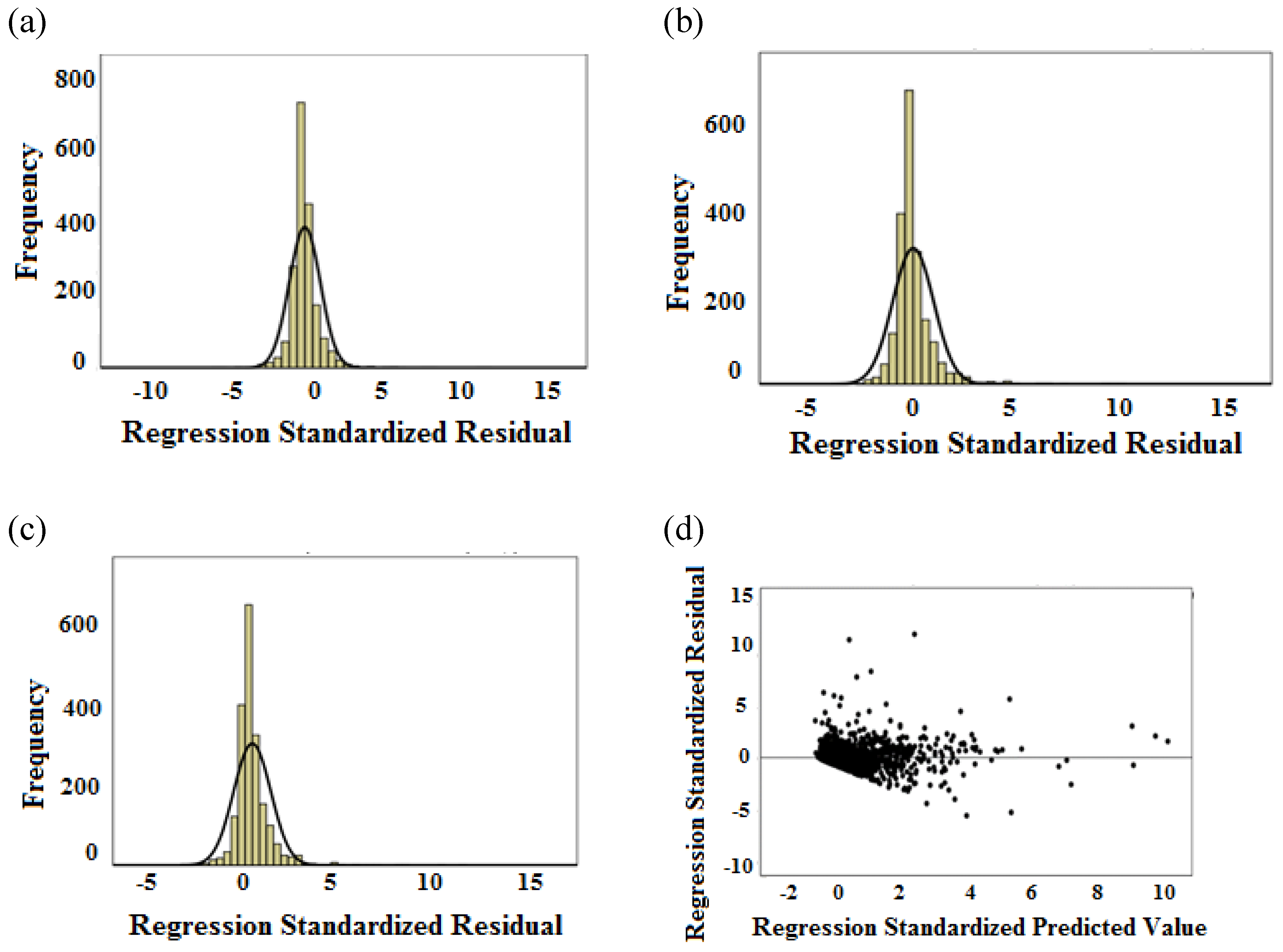
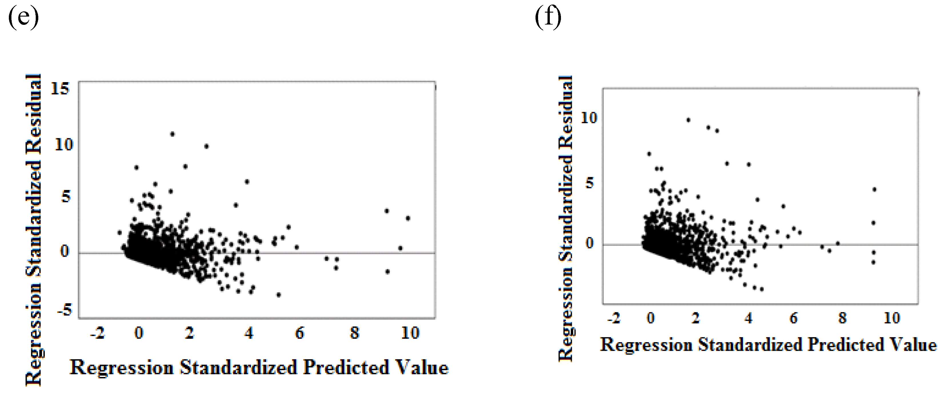
The normal distribution of residuals is illustrated with zero mean and constant variances for all three models in Figure 2a–c. Meanwhile, the fitted values plot with PM10 prediction model’s residuals show that the residuals are uncorrelated due to the residuals accumulating around the horizontal band, further indicating that the variance is constant and uncorrelated as depicted in Figure 2d–f. Unfortunately, more residuals dispersed away from the horizontal band as the prediction hour increased to the second to third hour of PM10 prediction time. Hence, this condition would hinder the best fit of the models, which reduced the precision of PM10 concentration forecasting.
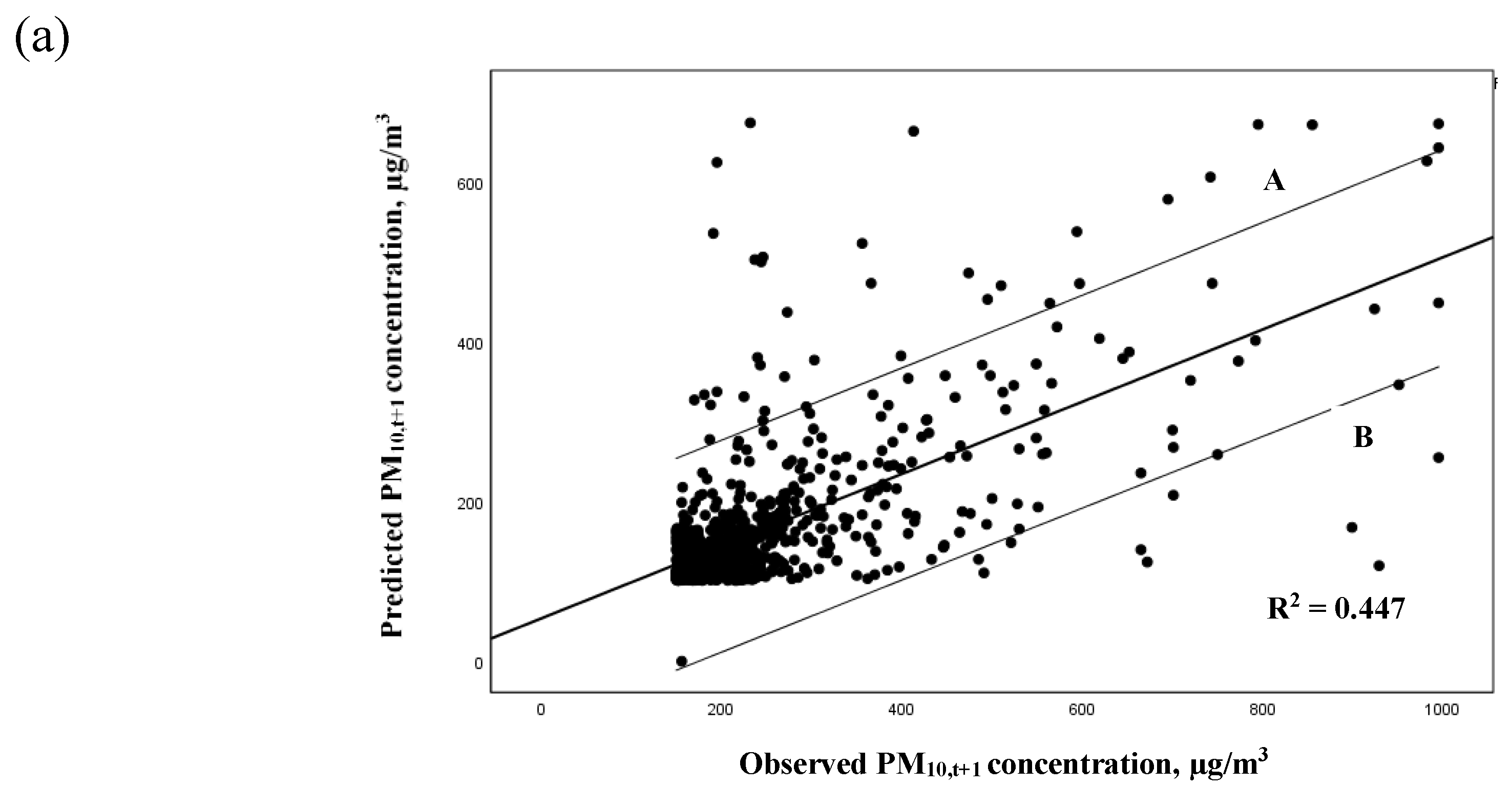
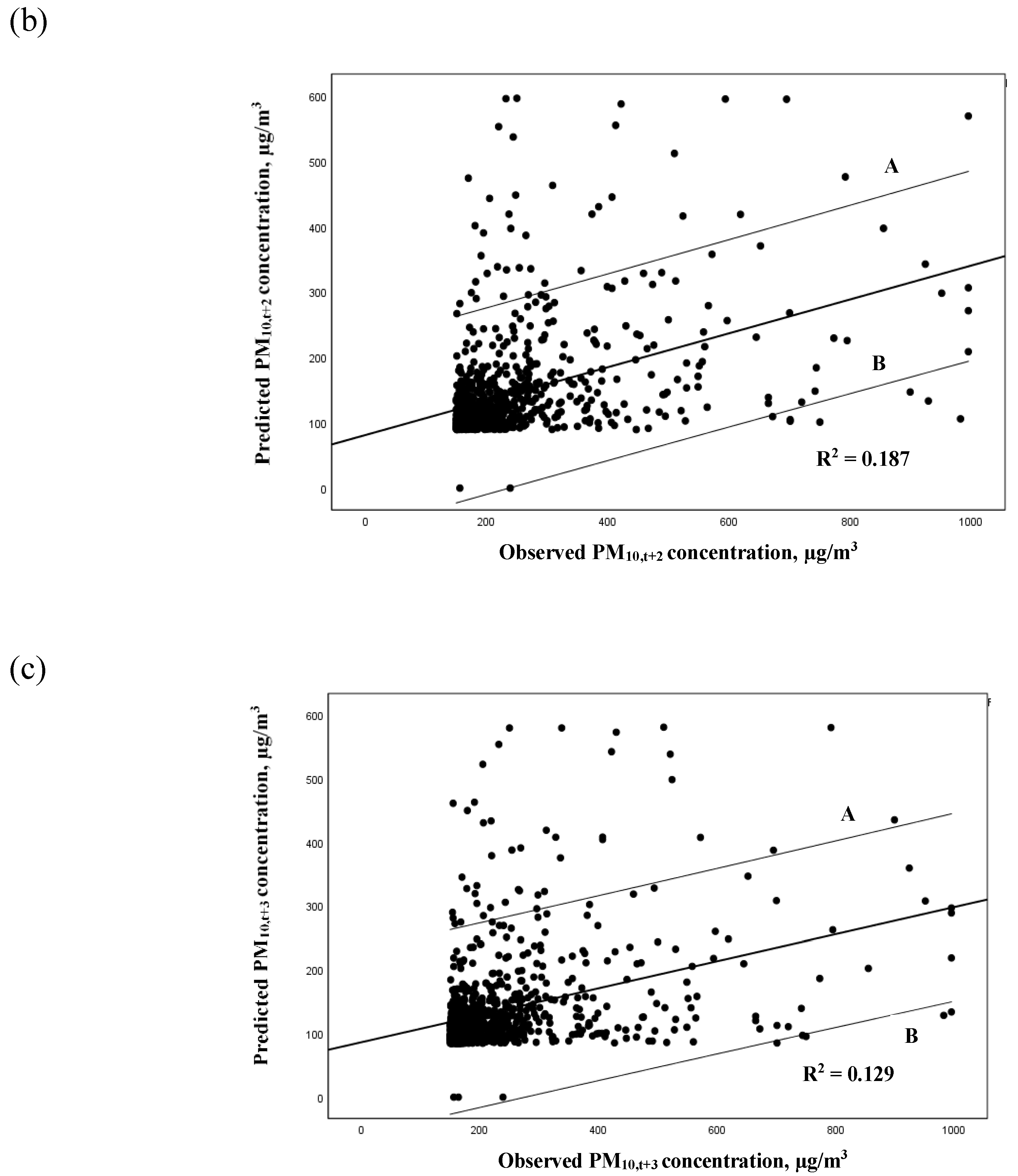
The predicted daily PM10 concentration was plotted against the observed PM10 concentration by prediction hour based on the 30% of haze chronology event data. Figure 3a–c illustrates the goodness-of-fit of the PM10 forecasting models in Malaysia. The regression lines drawn showing 95% confidence interval and most of the points were accumulated in between lines A and B, which were the upper and lower ranges of 95% confidence interval for the regression model. The accuracy of the predicted model for the next hour (PM10,t+1) was thus proven by having the highest R2 values of 0.447 compared to models PM10,t+2 (0.186) and PM10,t+3 (0.129). Hence, the increase of prediction hours of the models reduced their respective performance by increasing some of the errors of the prediction models, rendering it less precise [29,49].
The RMSE, NAE, and PA components were chosen in this study to measure the performance of the models. RMSE and NAE are considered as suitable indexes for determining model accuracy in which the model is noted as having a high accuracy when their values are close to zero, while the PA value is nearest to 1 [32,50,51]. According to a previous study [32], a comparison of the best statistical PM10 forecasting methods with the lowest values of RMSE and NAE and the highest PA value has been conducted to select the best-fit prediction model. Table 5 depicts the performance indicator values for all PM10 forecasting models in this study. It showed that the PM10,t+1 model yielded the lowest value of RMSE (126.728) and NAE (0.325), while it had the highest PA value (0.668) compared to the PM10,t+2, and PM10,t+3 models. Based on the results from this performance error and accuracy measures, the PM10,t+1 model provided better PM10 concentration forecasting capacity compared to model PM10,t+2, and model PM10,t+3 in Malaysia during transboundary haze events.

4. Conclusions

The maximum PM10 concentration was higher during transboundary haze events in the years 2013 and 2014 at 995 µg/m3 and the higher mean values of PM10 concentration was 274.860 µg/m3 (150–994 µg/m3) in the year 2005. Meanwhile, the lowest mean value obtained was 178.930 µg/m3 (150–497 µg/m3) in the year 2011. Next, the Spearman correlation analysis showed that CO was strongly and positively correlated with r = 0.512, p < 0.01. This was due to its higher emission through large-scale biomass combustion from neighboring countries. Furthermore, the best-fitted MLR model for PM10 prediction during transboundary haze events was PM10, t+1, which had a higher R2 of 0.447 compared to PM10,t+2 (0.186) and PM10,t+3 (0.129). On the other hand, PM10,t+1 was the best-fitted model with a higher accuracy of 0.668 and lower values of RMSE (126.728) and NAE (0.325) compared to models PM10,t+2 and PM10,t+3. The development of this model may thus aid the responsible parties in obtaining early information that can improve or initiate strategies in mitigating for better air quality.

Author Contributions

Conceptualization, S.A. and M.I.; methodology, S.A. and N.N.L.M.N.; software, W.N.W.M.; A.N.A.; validation, S.A. and N.N.L.M.N.; formal analysis, N.N.L.M.N.; writing—original draft preparation, N.N.L.M.N. and A.A.M.; writing—review and editing, S.A.; visualization, Z.T.A.R.; supervision, S.A., M.I. and W.N.W.M.; project administration, A.M.A.; funding acquisition, S.A., M.I. and A.M.A. All authors have read and agreed to the published version of the manuscript.

Funding

This research was funded by the Fundamental Research Grant Scheme for Research Acculturation of Early Career Researchers by the Malaysian Ministry of Education (RACER/1/2019/TK10/UMT//1) and the APC was funded by Research and Management Center, University Malaysia Terengganu.

Acknowledgments

The authors gratefully acknowledge the Malaysian Department of Environment for the air quality data.

Conflicts of Interest

The authors declare no conflict of interest.

References

  1. Thepnuan, D.; Chantara, S.; Lee, C.T.; Lin, N.H.; Tsai, Y.I. Molecular Markers for Biomass Burning Associated with the Characterization of PM2.5 and Component Sources during Dry Season Haze Episodes in Upper South East Asia. Sci. Total Environ. 2019, 658, 708–722. [Google Scholar] [CrossRef] [PubMed]
  2. Dotse, S.Q.; Dagar, L.; Petra, M.I.; Silva, L.C.D. Influence of Southeast Asian Haze Episodes on High PM10 Concentrations across Brunei Darussalam. Environ. Pollut. 2016, 219, 337–352. [Google Scholar] [CrossRef] [PubMed]
  3. Wen, Y.S.; Nor, A.F.M.; Fazilan, N.N.; Sulaiman, Z. Transboundary Air Pollution in Malaysia: Impact and Perspective on Haze. Nova J. Eng. Appl. Sci. 2016, 5, 1–11. [Google Scholar]
  4. Cheong, K.H.; Ngiam, N.J.; Morgan, G.G.; Pek, P.P.; Tan, B.Y.; Lai, J.W.; Koh, J.M.; Ong, M.E.H.; Ho, A.F.W. Acute Health Impacts of the Southeast Asian Transboundary Haze Problem—A Review. Int. J. Environ. Res. Public Health 2019, 16, 1–18. [Google Scholar] [CrossRef] [Green Version]
  5. Latif, M.T.; Othman, M.; Idris, N.; Juneng, L.; Abdullah, A.M.; Hamzah, W.P.; Khan, M.F.; Sulaiman, N.M.N.; Jewaratnam, J.; Aghamohammadi, N.; et al. Impact of Regional Haze towards Air Quality in Malaysia: A Review. Atmos. Environ. 2018, 177, 28–44. [Google Scholar] [CrossRef]
  6. Sahani, M.; Zainon, N.A.; Mahiyuddin, W.R.W.; Latif, M.T.; Hod, R.; Khan, M.F.; Tahir, N.M.; Chan, C.C. A Case-Crossover Analysis of Forest Fire Haze Events and Mortality in Malaysia. Atmos. Environ. 2014, 96, 257–265. [Google Scholar] [CrossRef]
  7. Forsyth, T. Public Concerns about Transboundary Haze: A Comparison of Indonesia, Singapore, and Malaysia. Glob. Environ. Chang. 2014, 25, 76–86. [Google Scholar] [CrossRef] [Green Version]
  8. Oanh, N.T.K.; Ly, B.T.; Tipayarom, D.; Manandhar, B.R.; Prapat, P.; Simpson, C.D.; Liu, L.J.S. Characterization of Particulate Matter Emission from Open Burning of Rice Straw. Atmos. Environ. 2011, 45, 493–502. [Google Scholar] [CrossRef] [Green Version]
  9. Li, Y.; Zheng, C.; Ma, Z.; Quan, W. Acute and Cumulative Effects of Haze Fine Particles on Mortality and the Seasonal Characteristics in Beijing, China, 2005–2013: A Time-Stratified Case-Crossover Study. Int. J. Environ. Res. Public Health 2019, 16, 1–11. [Google Scholar] [CrossRef] [Green Version]
  10. Sun, J.; Zhang, J.E.; Wang, C.; Duan, X.; Wang, Y. Escape or Stay? Effects of Haze Pollution on Domestic Travel: Comparative Analysis of Different Regions in China. Sci. Total Environ. 2019, 690, 151–157. [Google Scholar] [CrossRef]
  11. How, C.Y.; Ling, Y.E. The Influence of PM2.5 and PM10 on Air Pollution Index (API). Environmental Engineering, Hydraulics and Hydrology. In Proceedings of the Civil Engineering, Johor, Malaysia, 7–8 June 2016. [Google Scholar]
  12. Afroz, R.; Hassan, M.N.; Ibrahim, N.A. Review of Air Pollution and Health Impacts in Malaysia. Environ. Res. 2003, 92, 71–77. [Google Scholar] [CrossRef]
  13. Kusumaningtyas, S.D.A.; Aldrian, E. Impact of the June 2013 Riau Province Sumatera Smoke Haze Event on Regional Air Pollution. Environ. Res. Lett. 2016, 11, 075007. [Google Scholar] [CrossRef]
  14. Department of Environment, Malaysia. Malaysia Environmental Quality Report 2015. Available online: https://www.doe.gov.my/portalv1/en/ (accessed on 15 December 2019).
  15. Sun, J.; Wu, F.; Hu, B.; Tang, G.; Zhang, J.; Wang, Y. VOC Characteristics, Emissions and Contributions to SOA Formation during Hazy Episodes. Atmos. Environ. 2016, 141, 560–570. [Google Scholar] [CrossRef]
  16. Hoyle, C.R.; Boy, M.; Donahue, N.M.; Fry, J.L.; Glasius, M.; Guenther, A.; Hallar, A.G.; Huff Hartz, K.; Petters, M.D.; Petäjä, T.; et al. A Review of the Anthropogenic Influence on Biogenic Secondary Organic Aerosol. Atmos. Chem. Phys. 2011, 11, 321–343. [Google Scholar] [CrossRef] [Green Version]
  17. Jaafar, S.A.; Latif, M.T.; Razak, I.S.; Wahid, N.B.A.; Khan, M.F.; Srithawirat, T. Composition of Carbohydrates, Surfactants, Major Elements and Anions in PM2.5 during the 2013 Southeast Asia High Pollution Episode in Malaysia. Particuology 2018, 37, 119–126. [Google Scholar] [CrossRef]
  18. Othman, M.; Latif, M.T. Dust and Gas Emissions from Small-Scale Peat Combustion. Aerosol Air Qual. Res. 2013, 13, 1045–1059. [Google Scholar] [CrossRef]
  19. Koppmann, R.; Czapiewski, K.V.; Reid, J.S. A Review of Biomass Burning Emissions, Part I: Gaseous Emissions of Carbon Monoxide, Methane, Volatile Organic Compounds, and Nitrogen Containing Compounds. Atmos. Chem. Phys. Discuss. 2005, 5, 10455–10516. [Google Scholar] [CrossRef] [Green Version]
  20. Othman, J.; Sahani, M.; Mahmud, M.; Ahmad, M.K.S. Transboundary Smoke Haze Pollution in Malaysia: Inpatient Health Impacts and Economic Valuation. Environ. Pollut. 2014, 189, 194–201. [Google Scholar] [CrossRef]
  21. Hou, J.; An, Y.; Song, H.; Chen, J. The Impact of Haze Pollution on Regional Eco-Economic Treatment Efficiency in China: An Environmental Regulation Perspective. Int. J. Environ. Res. Public Health 2019, 16, 4059. [Google Scholar] [CrossRef] [Green Version]
  22. Rahman, H.A. Haze Phenomenon in Malaysia: Domestic or Transboudry Factor? Int. J. Chem. Environ. Biol. Sci. 2013, 1, 597–599. [Google Scholar]
  23. Song, Y.; Guo, S.; Zhang, M. Assessing Customers’ Perceived Value of the Anti-Haze Cosmetics under Haze Pollution. Sci. Total Environ. 2019, 685, 753–762. [Google Scholar] [CrossRef] [PubMed]
  24. Rembiesa, J.; Ruzgas, T.; Engblom, J.; Holefors, A. The Impact of Pollution on Skin and Proper Efficacy Testing for Anti-Pollution Claims. Cosmetics 2018, 5, 1–9. [Google Scholar] [CrossRef] [Green Version]
  25. Vierkötter, A.; Schikowski, T.; Ranft, U.; Sugiri, D.; Matsui, M.; Krämer, U.; Krutmann, J. Airborne Particle Exposure and Extrinsic Skin Aging. J. Investig. Dermatol. 2010, 130, 2719–2726. [Google Scholar] [CrossRef] [PubMed] [Green Version]
  26. Delavar, M.R.; Gholami, A.; Shiran, G.R.; Rashidi, Y.; Nakhaeizadeh, G.R.; Fedra, K.; Afshar, S.H. A Novel Method for Improving Air Pollution Prediction Based on Machine Learning Approaches: A Case Study Applied to the Capital City of Tehran. Int. J. Geo Inf. 2019, 8, 99. [Google Scholar] [CrossRef] [Green Version]
  27. Abdullah, S.; Ismail, M.; Fong, S.Y. Multiple Linear Regression (MLR) Models for Long Term PM10 Concentration Forecasting during Different Monsoon Seasons. J. Sustain. Sci. Manag. 2017, 12, 60–69. [Google Scholar]
  28. Mishra, D.; Goyal, P.; Upadhyay, A. Artificial Intelligence Based Approach to Forecast PM2.5 during Haze Episodes: A Case Study of Delhi, India. Atmos. Environ. 2015, 102, 239–248. [Google Scholar]
  29. Zounemat-Kermani, M. Hourly Predictive Levenberg-Marquardt ANN and Multi Linear Regression Models for Predicting of Dew Point Temperature. Meteorol. Atmos. Phys. 2012, 117, 181–192. [Google Scholar] [CrossRef]
  30. Yuen, F.S.; Abdullah, S.; Ismail, M. Forecasting of Particulate Matter (PM10) Concentration based on Gaseous Pollutants and Meteorological Factors for Different Monsoons of Urban Coastal Area in Terengganu. J. Sustain. Sci. Manag. 2018, 13, 3–17. [Google Scholar]
  31. Abdul-Wahab, S.A.; Bakheit, C.S.; Al-Alawi, S.M. Principal Component and Multiple Regression Analysis in Modelling of Ground-Level Ozone and Factors Affecting Its Concentrations. Environ. Model. Softw. 2005, 20, 1263–1271. [Google Scholar] [CrossRef]
  32. Abdullah, S.; Ismail, M.; Ahmed, A.N.; Abdullah, A.M. Forecasting Particulate Matter Concentration Using Linear and Non-Linear Approaches for Air Quality Decision Support. Atmosphere 2019, 10, 667. [Google Scholar] [CrossRef] [Green Version]
  33. Abdullah, S.; Ismail, M.; Fong, S.Y.; Ahmed, A.N. Evaluation for Long Term PM10 Concentration Forecasting Using Multi Linear Regression (MLR) and Principal Component Regression (PCR) Models. EnvironmentAsia 2016, 9, 101–110. [Google Scholar]
  34. Hashim, N.I.M.; Noor, N.M. Variations of Particulate Matter (PM10) Concentration during Haze Episodes in Malaysia. In Proceedings of the 2017 Bangkok International Intellectual Property, Invention, Innovation and Technology Exposition, Bangkok, Thailand, 4 January 2017. [Google Scholar]
  35. Awang, N.R.; Ramli, N.A.; Yahaya, A.S.; Elbayoumi, M. Multivariate Methods to Predict Ground Level Ozone during Daytime, Nighttime, and Critical Conversion Time in Urban Areas. Atmos. Pollut. Res. 2015, 6, 726–734. [Google Scholar] [CrossRef]
  36. Awang, N.R.; Elbayoumi, M.; Ramli, N.A.; Yahaya, A.S. Diurnal Variations of Ground-Level Ozone in Three Port Cities in Malaysia. Air Qual. Atmos. Health 2016, 9, 25–39. [Google Scholar] [CrossRef]
  37. Latif, M.T.; Dominick, D.; Ahamad, F.; Khan, M.F.; Juneng, L.; Hamzah, F.M.; Nadzir, M.S.M. Long Term Assessment of Air Quality from a Background Station on the Malaysian Peninsula. Sci. Total Environ. 2014, 482–483, 336–348. [Google Scholar] [CrossRef] [PubMed]
  38. Banan, N.; Latif, M.T.; Juneng, L.; Ahamad, F. Characteristics of Surface Ozone Concentrations at Stations with Different Backgrounds in the Malaysian Peninsula. Aerosol Air Qual. Res. 2013, 13, 1090–1106. [Google Scholar] [CrossRef] [Green Version]
  39. Kang, H. The Prevention and Handling of the Missing Data. Korean J. Anesthesiol. 2013, 64, 402–406. [Google Scholar] [CrossRef] [PubMed]
  40. Abdullah, S.; Ismail, M.; Samat, N.N.A.; Ahmed, A.N. Modelling Particulate Matter (PM10) Concentration in Industrialized Area: A Comparative Study of Linear and Nonlinear Algorithms. ARPN J. Eng. Appl. Sci. 2018, 13, 8227–8235. [Google Scholar]
  41. Roy, K.; Ambure, P. The Double Cross-Validation Software Tool for MLR QSAR Model Development. Chemom. Intell. Lab. Syst. 2016, 159, 108–126. [Google Scholar] [CrossRef]
  42. Ul-Saufie, A.Z.; Yahya, A.S.; Ramli, N.A.; Hamid, N.A. Comparison Between Multiple Linear Regression and Feed Forward Back Propagation Neural Network Models for Predicting PM10 Concentration Level Based On Gaseous and Meteorological Parameters. Int. J. Appl. Sci. Technol. 2011, 1, 42–49. [Google Scholar]
  43. Department of Environment, Malaysia. Malaysia Environmental Quality Report 2016. Available online: https://www.doe.gov.my/portalv1/en/ (accessed on 15 December 2019).
  44. Latif, M.T.; Abidin, E.Z.; Praveena, S.M. The Assessment of Ambient Air Pollution Trend in Klang Valley. World Environ. 2015, 5, 1–11. [Google Scholar]
  45. Rajab, J.M.; Tan, K.C.; Lim, H.S.; Matjafri, M.Z. Investigation on the Carbon Monoxide Pollution over Peninsular Malaysia Caused by Indonesia Forest Fires from AIRS Daily Measurement. Adv. Air Pollut. 2011, 8, 115–136. [Google Scholar]
  46. Bartington, S.E.; Bakolis, I.; Devakumar, D.; Kurmi, O.P.; Gulliver, J.; Chaube, G.; Manandhar, D.S.; Saville, N.M.; Costello, A.; Osrin, D.; et al. Patterns of Domestic Exposure to Carbon Monoxide and Particulate Matter in Households Using Biomass Fuel in Janakpur, Nepal. Environ. Pollut. 2017, 220, 38–45. [Google Scholar] [CrossRef] [PubMed] [Green Version]
  47. Yusof, K.M.K.K.; Azid, A.; Sani, M.S.A.; Samsudin, M.S.; Amin, S.N.M.; Rani, N.L.A.; Jamalani, M.A. The Evaluation on Artificial Neural Networks (ANN) and Multiple Linear Regressions (MLR) Models over Particulate Matter (PM10) Variability during Haze and Non-Haze Episodes: A Decade Case Study. Malays. J. Fundam. Appl. Sci. 2019, 15, 164–172. [Google Scholar] [CrossRef]
  48. Petetin, H.; Sauvage, B.; Parrington, M.; Clark, H.; Fontaine, A.; Athier, G.; Blot, R.; Boulanger, D.; Cousin, J.M.; Nédélec, P.; et al. The Role of Biomass Burning as Derived from the Tropospheric CO Vertical Profiles Measured by IAGOS Aircraft in 2002–2017. Atmos. Chem. Phys. 2018, 18, 17277–17306. [Google Scholar] [CrossRef] [Green Version]
  49. Wang, Z.; Wang, Y.; Zeng, R.; Srinivasan, R.S.; Ahrentzen, S. Random Forest Based Hourly Building Energy Prediction. Energy Build. 2018, 171, 11–25. [Google Scholar] [CrossRef]
  50. Vakili, M.; Sabbagh-Yazdi, S.R.; Khosrojerdi, S.; Kalhor, K. Evaluating the Effect of Particulate Matter Pollution on Estimation of Daily Global Solar Radiation Using Artificial Neural Network Modeling Based on Meteorological Data. J. Clean. Prod. 2017, 141, 1275–1285. [Google Scholar] [CrossRef]
  51. Domańska, D.; Wojtylak, M. Explorative Forecasting of Air Pollution. Atmos. Environ. 2014, 92, 19–30. [Google Scholar] [CrossRef]
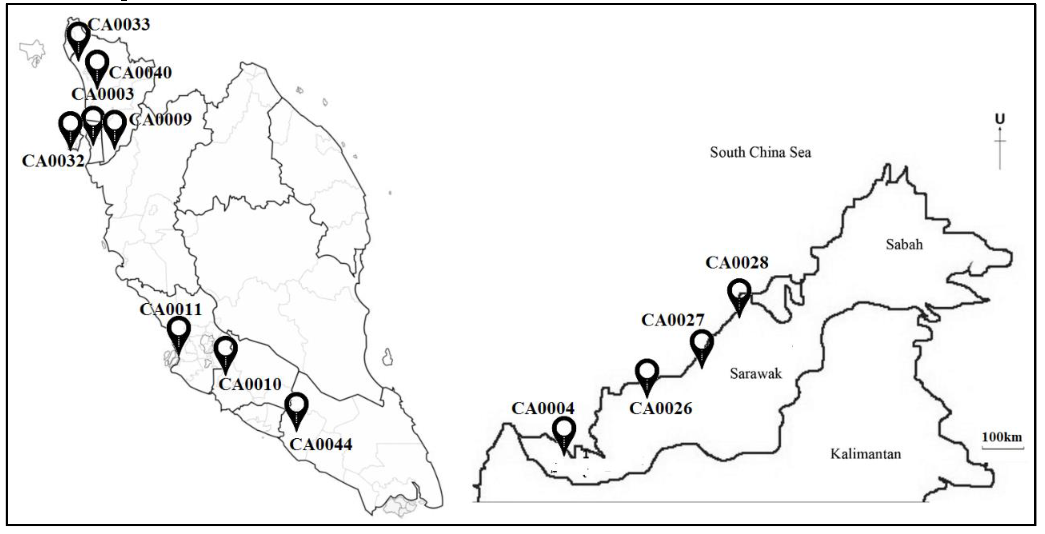
Figure 1. Study Areas.
Atmosphere 11 00289 g001
Figure 2. (a) Standardized residual analysis of PM10,t+1, (b) standardized residual analysis of PM10,t+2, (c) standardized residual analysis of PM10,t+3, (d) testing assumption of variance and uncorrelated with mean equal to zero for model PM10,t+1, (e) testing assumption of variance and uncorrelated with mean equal to zero for model PM10,t+2, (f) testing assumption of variance and uncorrelated with mean equal to zero for model PM10,t+3.
Atmosphere 11 00289 g002aAtmosphere 11 00289 g002b
Figure 3. Scatter plot of predicted PM10 concentration (µg/m3) against observed PM10 concentration (µg/m3) for (a) PM10,t+1 model, (b) PM10,t+2 model, and (c) PM10,t+3 model.
Atmosphere 11 00289 g003aAtmosphere 11 00289 g003b
Table 1. Selected air monitoring stations in Malaysia affected during haze events.
ClassificationStation IDLocationLatitudeLongitude
IndustrialCA0003Cenderawasih Primary School, PeraiN05° 23.470E100° 23.213
IndustrialCA0004Medical Store, Kuching, SarawakN01° 33.734E110° 23.329
Sub-UrbanCA0009Seberang Jaya II Primary School, Perai, PenangN05° 23.890E100° 24.194
IndustrialCA0010Taman Semarak (Phase II), Nilai, Negeri SembilanN02° 49.246E101° 48.877
UrbanCA0011Raja Zarina Secondary School, Klang, SelangorN03° 00.620E101°24.484
Sub-UrbanCA0026Sibu Police Main Office, SarawakN02° 18.856E111° 49.906
Sub-UrbanCA0027Bintulu Police Station, SarawakN03° 10.587E113° 02.433
Sub-UrbanCA0028Dato Permaisuri Secondary School, Miri, SarawakN04° 25.456E114° 00.731
Sub-UrbanCA0032Langkawi Sport Complex, Langkawi, KedahN06° 19.903E099° 51.517
Sub-UrbanCA0033MADA, Behor Temak, Kangar, PerlisN06° 25.424E100° 11.046
UrbanCA0040Islamic Religious Secondary School, Mergong, Alor Setar, KedahN06° 08.218E100° 20.880
Sub-UrbanCA0044Vocational Secondary School, Muar, JohorN02° 03.715E102° 35.587
Table 2. Summary of descriptive statistics during periodic haze events in Malaysia.
Descriptive Statistical2005
(N = 369)
2006
(N = 918)
2010
(N = 61)
2011
(N = 260)
2012
(N = 402)
2013
(N = 236)
2014
(N = 613)
Mean (µg/m3)274.860199.100275.100178.930204.270260.650233.520
Median (µg/m3)237.000180.000196.000168.000181.000210.000187.000
Std. Deviation (µg/m3)136.10356.435170.71737.29963.071141.508131.163
Variance18524.0963184.95529144.3231392.1803977.93120024.50017203.855
Minimum (µg/m3)150.000150.000150.000150.000150.000150.000150.000
Maximum (µg/m3)994.000573.000866.000497.000533.000995.000995.000
Table 3. Spearman correlation of PM10 between meteorological factors and other gaseous pollutants during periodic haze events.
ParameterPM10WSTRHNOSO2NO2O3CO
PM101.000.0430.055 *−0.076 **−0.0250.131 **0.059 **0.046 *0.512 **
WS 1.000.517 **−0.537 **−0.380 **−0.029−0.372 **0.615 **−0.206 **
T 1.00−0.820 **−0.259 **0.050 *−0.088 **0.621 **0.006
RH 1.000.230 **−0.196 **0.003−0.590 **−0.038
NO 1.000.259 **0.617 **−0.671 **0.325 **
SO2 1.000.458 **−0.141 **0.356 **
NO2 1.00−0.443 **0.437 **
O3 1.00−0.243 **
CO 1.00
Note ** Correlation is significant at the 0.01 level (2-tailed), * Correlation is significant at the 0.05 level (2-tailed).
Table 4. Model summary for PM10 concentration forecasting during transboundary haze events in Malaysia.
Prediction HourModelR2VIFDurbin-Watson
Hour 1, t+1PM10,t+1 = 0.004 + 0.673 PM10 + 0.230 CO − 0.057 NO0.6381.275–2.1492.125
Hour 2, t+2PM10,t+2 = 0.019 + 0.597 PM10 + 0.141 CO − 0.053 NO0.4521.275–2.1491.201
Hour 3, t+3PM10,t+3 = 0.069 + 0.586 PM10 − 0.047 RH − 0.046 O30.3531.006–1.6290.932
Table 5. Summary of performance indicator for all PM10 forecasting models during the transboundary haze events.
Prediction HourRMSENAEPA
Hour 1, t+1126.7280.3250.668
Hour 2, t+2156.5060.4030.431
Hour 3, t+3164.9780.4290.359