Quantitative Fluxes of the Greenhouse Gases CH4 and CO2 from the Surfaces of Selected Polish Reservoirs


Abstract
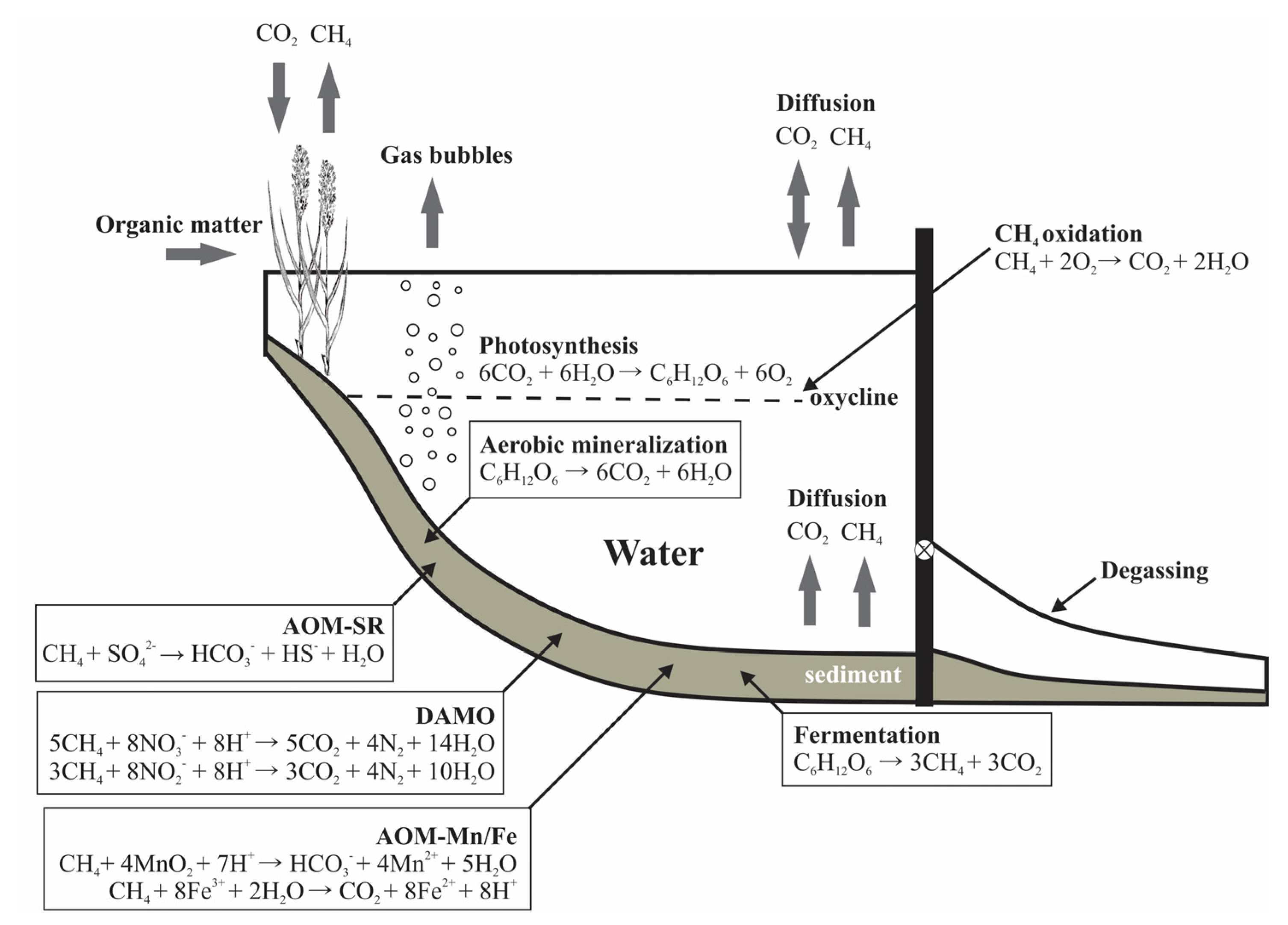
1. Introduction
2. Materials and Methods
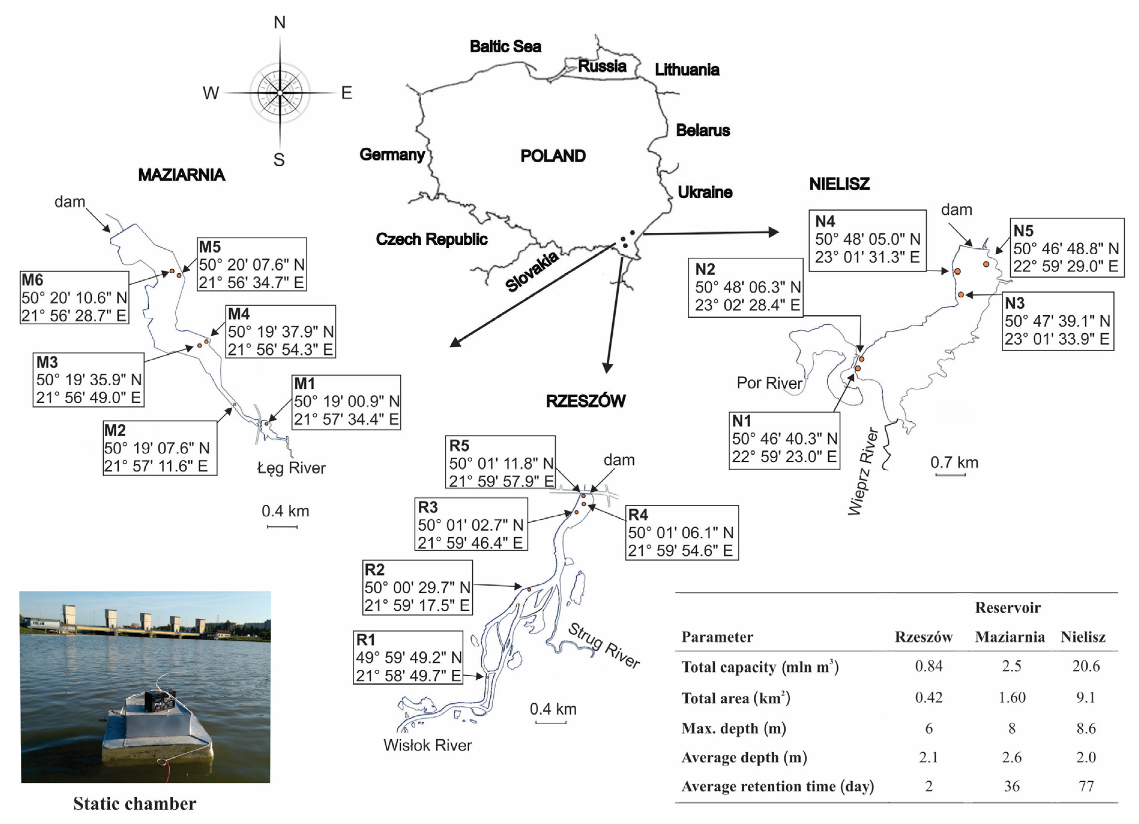
2.1. Research Periods and Sites
2.2. Measurement of CH4 and CO2 Fluxes at the Water–Air Interface
2.3. Sediment Analysis
2.4. Statistical Calculations
3. Results
3.1. Sediment Characteristics
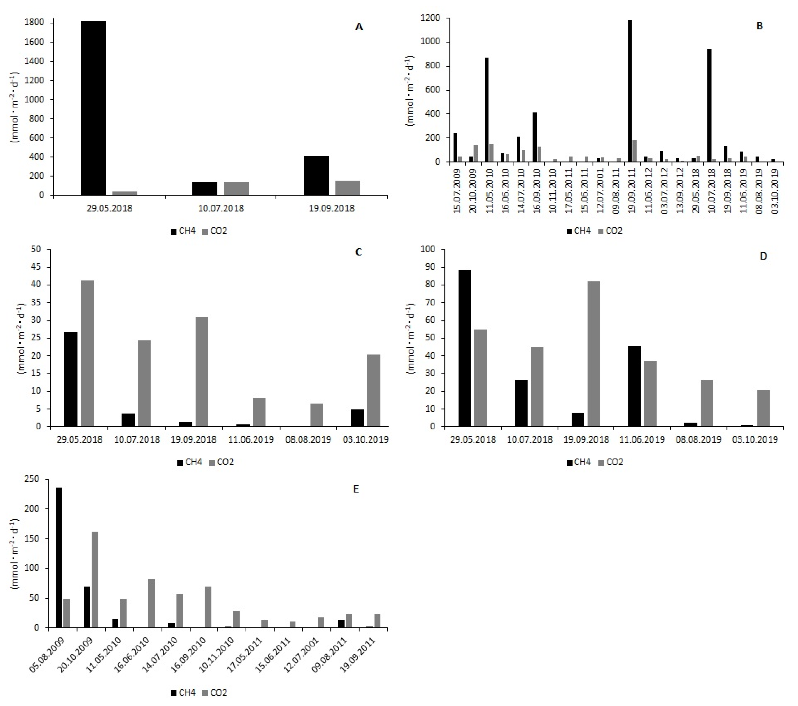
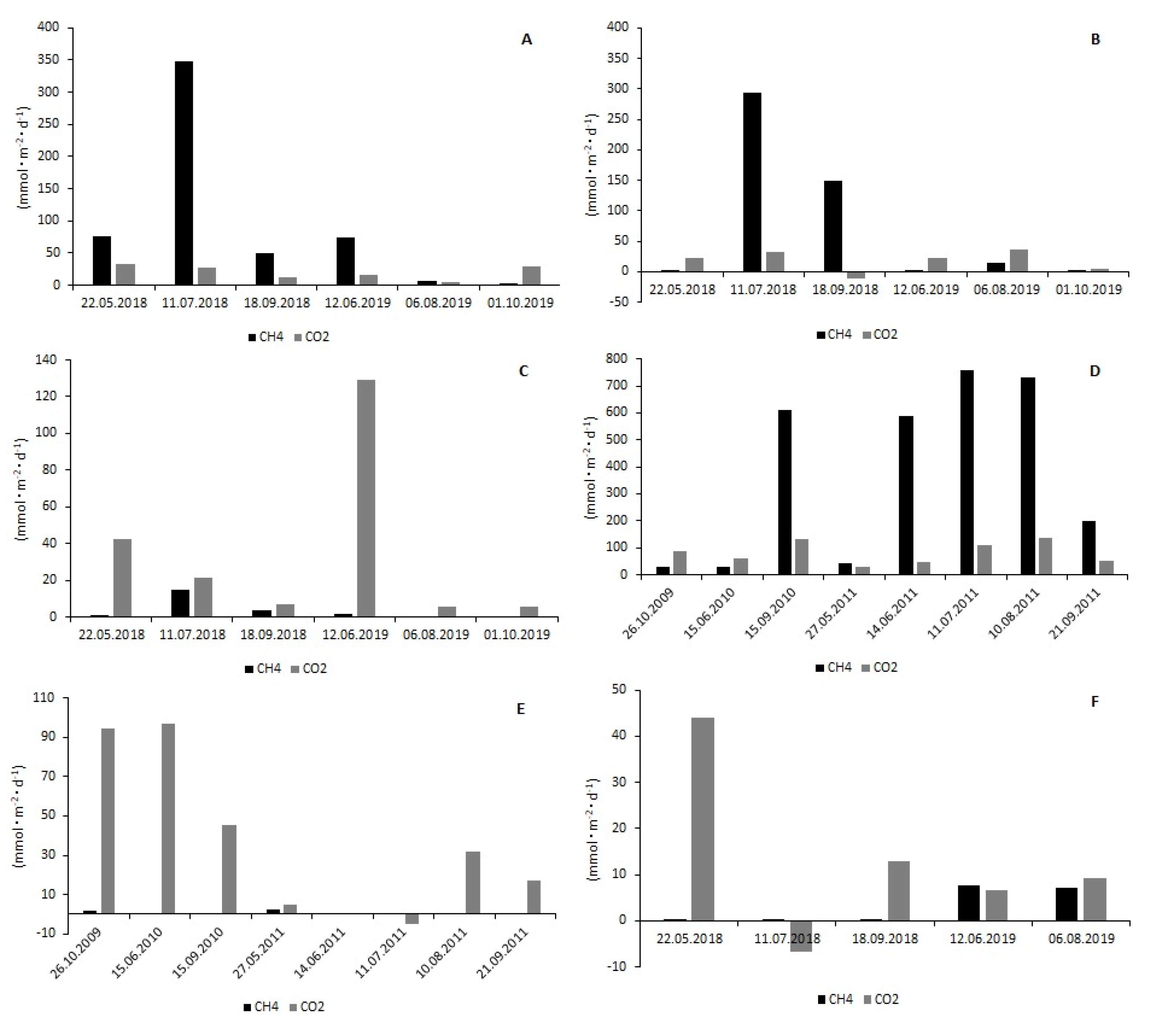
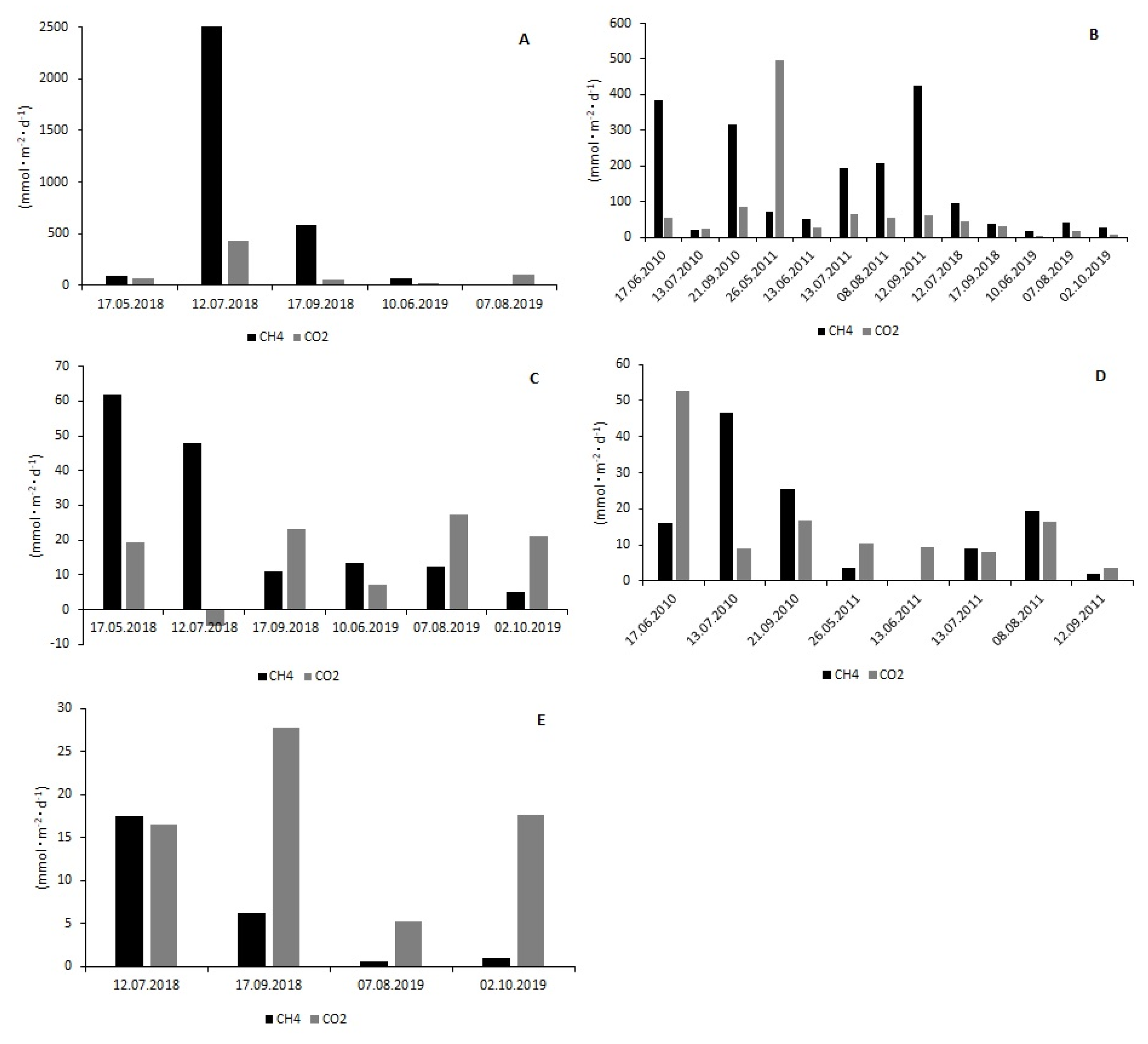
3.2. CH4 and CO2 Fluxes at the Water–Air Interface
4. Discussion

| Reservoir/Lake | CH4 | CO2 | Source |
|---|---|---|---|
| (mmol·m−2·d−1) | (mmol·m−2·d−1) | ||
| Boreal Zone | |||
| Grand Rapids (Canada) | −0.004–1.73 (0.036) | −8.00–165.00 (14.00) | [57] |
| Jenpeg (Canada) | −0.004–0.68 (0.069) | −21.00–48.00 (7.00) | [57] |
| Kettle (Canada) | −0.012–0.06 (0.000) | −16.00–128.00 (12.00) | [57] |
| McArthur (Canada) | −0.002–0.45 (0.002) | −24.00–81.00 (8.00) | [57] |
| EM-1 (Canada) | 0.00–0.51 (0.048) | 0.00–447.00 (55.00) | [57] |
| RDP (Canada) | 0–0.40 (0.031) | −5.00–213.00 (15.00) | [57] |
| LG-2 (Canada) | 0–0.16 (0.009) | 1.00–148.00 (15.00) | [57] |
| Lokka (Finland) | 0.33–7.40 (1.44) | 11.00–73.00 (34.50) | [3] |
| Porttipahta (Finland) | 0.16–0.30 (0.22) | 20.00–52.00 (35.00) | [3] |
| Temperate Zone | |||
| Wohlen (Switzerland) | (53.44) | [44] | |
| Gruyere (Switzerland) | (0.009) | (22.25) | [58] |
| Lungern (Switzerland) | (0.008) | (5.50) | [58] |
| Sihl (Switzerland) | (0.013) | (25.00) | [58] |
| Luzzone (Switzerland) | (0.008) | (32.14) | [58] |
| Solina (Poland) | −20.78–14.73 | [59] | |
| F. D. Roosevelt (USA) | 0.10–0.51 (0.20) | −19.36–5.70 (−10.5) | [35] |
| Dworshak (USA) | 0.04–0.93 (0.21) | −51.77–−16.36 (−27.16) | [35] |
| Wallula (USA) | 0.22–1.06 (0.56) | −37.02–24.09 (−7.93) | [35] |
| Shasta (USA) | −0.09–1.83 (0.59) | 7.98–48.86 (28.34) | [35] |
| Oroville (USA) | 0.07–0.66 (0.26) | 6.05–55.23 (23.32) | [35] |
| Eagle Creek (USA) | (0.66) | (45.68) | [60] |
| 5 lakes (Netherlands) | 2.10–27.15 (5.85) | −3.27–67.58 (33.60) | [51] |
| Three Gorges (China) | 0–0.99 (0.24) | [45] | |
| Three Gorges (China) | (0.08) | (56.96) | [48] |
| Three Gorges (China) | (89.07) | [61] | |
| Shuibuya (China) | (0.08) | (85.00) | [62] |
| Temperate reservoirs | 0.63–5.00 (1.25) | 17.05–70.45 (31.82) | [27] |
| Reservoir | CH4 | CO2 | Source |
|---|---|---|---|
| (mmol·m−2·d−1) | (mmol·m−2·d−1) | ||
| Subtropical zone | |||
| Gold Creek (Australia) | 0.41–306.25 | [67] | |
| Tropical zone | |||
| Balbina (Brazil) | (0.31) | (36.36) | [53] |
| Balbina (Brazil) | 28.59–710.75 (314.66) | [68] | |
| Miranda (Brazil) | 1.25–296.72 (16.40) | 0.36–1390.51 (113.18) | [69] |
| Tres Marias (Brazil) | 0.06–90.38 (23.89) | −282.64–0.94 (-3.23) | [69] |
| Barra Bonita (Brazil) | 0.19–3.13 (1.20) | 36.68–759.64 (146.23) | [69] |
| Segredo (Brazil) | 0.00–5.81 (0.62) | 0.00–1064.98 (108.84) | [69] |
| Xingó (Brazil) | 0.21–9.81 (1.87) | 0.66–2027.34 (223.57) | [69] |
| Samuel (Brazil) | 0.31–152.63 (11.48) | 52.57–371.56 (183.80) | [69] |
| Tucurui (Brazil) | 0.00–6.81 (12.84) | 29.86–3243.73 (237.11) | [69] |
| Itaipu (Brazil) | 0.09–3.13 (0.81) | −60.14–181.38 (27.39) | [69] |
| Serra da Messa (Brazil) | −0.24–63.21 (7.56) | −14.34–134.14 (29.91) | [69] |
| Funil (Brazil) | 0.04–13.50 (0.99) | [34] | |
| Santo Antonio (Brazil) | 0.33–72.10 (9.30) | [34] | |
| Petit Saut (French Guyana) | 0.31–237.50 (71.25) | 13.18–238.59 (101.36) | [70] |
| Nam Ngum (Laos) | 0.10–0.60 | −21.20–−2.70 | [71] |
| Nam Leuk (Laos) | 0.80–11.90 | −10.60–38.20 | [71] |
| Tropical reservoir | 1.25–93.75 (18.75) | 10.23–231.82 (79.55) | [27] |
5. Summary
Supplementary Materials
Funding
Conflicts of Interest
References
- IPCC. Climate Change 2014: Mitigation of Climate Change. Contribution of Working Group III to the Fifth Assessment Report of the Intergovernmental Panel on Climate Change; Edenhofer, O., Pichs-Madruga, R., Sokona, Y., Farahani, E., Kadner, S., Seyboth, K., Adler, A., Baum, I., Brunner, S., Eickemeier, P., et al., Eds.; Cambridge University Press: Cambridge, UK, 2014. [Google Scholar]
- Conrad, R. Control of microbial methane production in wetland rice fields. Nutr. Cycl. Agroecosyst. 2002, 64, 59–69. [Google Scholar] [CrossRef]
- Huttunen, J.T.; Alm, J.; Liikanen, A.; Juutinen, S.; Larmola, T.; Hammar, T.; Silvola, J.; Martikainen, P.J. Fluxes of methane, carbon dioxide and nitrous oxide in boreal lakes and potential anthropogenic effects on the aquatic greenhouse gas emission. Chemosphere 2003, 52, 609–621. [Google Scholar] [CrossRef]
- Bergier, I.; Novo, E.M.L.; Ramos, F.M.; Mazzi, E.A.; Rasera, M.F.F.L. Carbon dioxide and methane fluxes in the littoral zone of a tropical Savanna Reservoir (Corumba, Brazil). Oecologia Aust. 2011, 15, 666–681. [Google Scholar] [CrossRef]
- Gruca-Rokosz, R.; Tomaszek, J.A.; Czerwieniec, E. Methane emission from the Nielisz Reservoir. Environ. Prot. Eng. 2011, 37, 101–109. [Google Scholar]
- Zhao, Y.; Wu, B.F.; Zeng, Y. Spatial and temporal patterns of greenhouse gas emissions from Three Gorges Reservoir of China. Biogeosciences 2013, 10, 1219–1230. [Google Scholar] [CrossRef]
- Sepulveda-Jauregui, A.; Walter Anthony, K.M.; Martinez-Cruz, K.; Greene, S. Methane and carbon dioxide emissions from 40 lakes along a north–south latitudinal transect in Alaska. Biogeosci. Discuss. 2014, 11, 13251–13307. [Google Scholar] [CrossRef]
- Borhan, M.S.; Capareda, S.C.; Mukhtar, S.; Faulkner, W.B.; McGee, R.; Parnell, C.B. Greenhouse Gas Emissions from Ground Level Area Sources in Dairy and Cattle Feedyard Operations. Atmosphere 2011, 2, 303. [Google Scholar] [CrossRef]
- Różański, K.; Nęcki, J.; Chmura, Ł.; Śliwka, I.; Zimnoch, M.; Bielewski, J.; Gałkowski, M.; Bartyzel, J.; Rosiek, J. Anthropogenic changes of CO2, CH4, N2O, CFCl3, CF2Cl2, CCl2FCClF2, CHCl3, CH3CCl3, CCl4, SF6 and SF5CF3 mixing ratios in the atmosphere over southern Poland. Geol. Q. 2014, 58, 673–684. [Google Scholar] [CrossRef]
- Sun, W.; Deng, L.; Wu, G.; Wu, L.; Han, P.; Miao, Y.; Yao, B. Atmospheric monitoring of methane in Beijing using a mobile observatory. Atmosphere 2019, 10, 554. [Google Scholar] [CrossRef]
- Belikov, D.; Arshinov, M.; Belan, B.; Davydov, D.; Fofonov, A.; Sasakawa, M.; Machida, T. Analysis of the diurnal, weekly, and seasonal cycles and annual trends in atmospheric CO2 and CH4 at Tower Network in Siberia from 2005 to 2016. Atmosphere 2019, 10, 689. [Google Scholar] [CrossRef]
- Froelich, P.N.; Klinkhammer, G.P.; Bender, M.L.; Luedtke, N.A.; Heath, G.R.; Cullen, D.; Dauphin, P.; Maynard, V. Early oxidation of organic matter in pelagic sediments of the eastern equatorial Atlantic: Suboxic diagenesis. Geochim. Cosmochim. Acta 1979, 43, 1075–1090. [Google Scholar] [CrossRef]
- Guérin, F.; Abril, G. Significance of pelagic aerobic methane oxidation in the methane and carbon budget of tropical reservoir. J. Geophys. Res. 2007, 112, G03006. [Google Scholar] [CrossRef]
- Jędrysek, M.O.; Hałas, S.; Pieńkos, T. Carbon isotopic composition of early-diagenetic methane: Variations with sediments depth. Ann. Univ. Mariae Curie Skłodowska 2014, LXIX, 29–52. [Google Scholar]
- Boon, P.I. Carbon cycling in Australian wetlands: The importance of methane. Verh. Internat. Verein. Limnol. 2000, 27, 37–50. [Google Scholar] [CrossRef]
- Chen, H.; Wu, N.; Yao, S.; Gao, Y.; Zhu, D.; Wang, Y.; Xions, W.; Yuan, X. High methane emissions from a littoral zone on the Qinghai-Tibetan Plateau. Atmos. Environ. 2009, 43, 4995–5000. [Google Scholar] [CrossRef]
- Fearnside, P.M. Greenhouse gas emissions from hydroelectric dams: Controversies provide a springboard for rethinking a supposedly “clean” energy source—An editorial comment. Clim. Chang. 2004, 66, 1–8. [Google Scholar] [CrossRef]
- Barros, N.; Cole, J.J.; Tranvik, L.J.; Prairie, Y.T.; Bastviken, D.; Huszar, V.L.M.; Del Giorgio, P.; Roland, F. Carbon emission from hydroelectric reservoirs linked to reservoir age and latitude. Nat. Geosci. 2011, 4, 593–596. [Google Scholar] [CrossRef]
- Juutinen, S. Methane Fluxes and Their Environmental Controls in the Littoral Zone of Boreal Lakes. Ph.D. Thesis, University of Joensuu, Joensuu, Finland, 2004. [Google Scholar]
- Narvenkar, G.; Naqvi, S.W.A.; Kurian, S.; Shenoy, D.M.; Pratihary, A.K.; Naik, H.; Patil, S.; Sarkar, A.; Gauns, M. Dissolved methane in Indian freshwater reservoirs. Environ. Monit. Assess. 2013, 185, 6989–6999. [Google Scholar] [CrossRef]
- Schubert, C.J.; Vazquez, F.; Lösekann-Behrens, T.; Knittel, K.; Tonolla, M.; Boetius, A. Evidence for anaerobic oxidation of methane in sediments of a freshwater system (Lago di Cadagno). FEMS Microbiol. Ecol. 2011, 76, 26–38. [Google Scholar] [CrossRef]
- Sivan, O.; Adler, M.; Pearson, A.; Gelman, F.; Bar-Or, I.; John, S.G.; Eckert, W. Geochemical evidence for iron-mediated anaerobic oxidation of methane. Limnol. Oceanogr. 2011, 56, 1536–1544. [Google Scholar] [CrossRef]
- He, Z.; Zhang, Q.; Feng, Y.; Luo, H.; Pan, X.; Gadd, G.M. Microbiological and environmental significance of metal-dependent anaerobic oxidation of methane. Sci. Total Environ. 2018, 610–611, 759–768. [Google Scholar] [CrossRef] [PubMed]
- Martinez-Cruz, K.; Sepulveda-Jauregui, A.; Casper, P.; Walter Anthony, K.; Smemo, K.A.; Thalasso, F. Ubiquitous and significant anaerobic oxidation of methane in freshwater lake sediments. Water Res. 2018, 144, 332–340. [Google Scholar] [CrossRef] [PubMed]
- Yang, Y.; Chen, J.; Li, B.; Liu, Y.; Xie, S. Anaerobic methane oxidation potential and bacteria in freshwater lakes: Seasonal changes and the influence of trophic status. Syst. Appl. Microbiol. 2018, 41, 650–657. [Google Scholar] [CrossRef] [PubMed]
- Szal, D.; Gruca-Rokosz, R. Denitrification-dependent anaerobic oxidation of methane in freshwater sediments of reservoirs in SE Poland. J. Ecol. Eng. 2019, 20, 218–227. [Google Scholar] [CrossRef]
- St Louis, V.L.; Kelly, C.A.; Duchemin, E.; Rudd, J.W.M.; Rosenberg, D.M. Reservoir surfaces as sources of greenhouse gases to the atmosphere: A global estimate. BioScience 2000, 50, 766–775. [Google Scholar] [CrossRef]
- Guérin, F.; Abril, G.; Richard, S.; Burban, B.; Reynouard, C.; Seyler, P.; Delmas, R. Methane and carbon dioxide emission from tropical reservoirs: Significance of downstream rivers. Geophys. Res. Lett. 2006, 33, L21407. [Google Scholar] [CrossRef]
- Raymond, P.A.; Hartman, J.; Lauerwald, R.; Sobek, S.; Mcdonald, C.; Hoover, M.; Butman, D.; Striegl, R.; Mayorga, E.; Humborg, C.; et al. Global carbon dioxide emissions from inland waters. Nature 2013, 503, 355. [Google Scholar] [CrossRef]
- Tranvik, L.J.; Downing, J.A.; Weyhenmeyer, G.A. Lakes and reservoirs as regulators of carbon cycling and climate. Limnol. Oceanogr. 2009, 54, 2298–2314. [Google Scholar] [CrossRef]
- Bastviken, D.; Tranvik, L.J.; Downing, J.A.; Crill, P.M.; Enrich-Prast, A. Freshwater methane emissions offset the continental carbon sink—supporting information. Science 2011, 331, 50. [Google Scholar] [CrossRef]
- Gruca-Rokosz, R. Dynamics of Carbon Greenhouse Gases in Reservoirs: Production Pathways, Emission to the Atmosphere; Printing House of Rzeszów University of Technology: Rzeszów, Poland, 2015. [Google Scholar]
- Koszelnik, P.; Tomaszek, J.; Gruca-Rokosz, R. Carbon and nitrogen and their elemental and isotopic ratios in the bottom sediment of the Solina-Myczkowce complex of reservoirs. Oceanol. Hydrobiol. Stud. 2008, 37, 71–78. [Google Scholar] [CrossRef]
- Grandin, K. Variations of CH4 Emissions within and between Hydroelectric Reservoirs in Brazil. Master’ Thesis, Uppsala University, Uppsala, Sweden, 2012. [Google Scholar]
- Soumis, N.; Duchemin, E.; Canuel, R.; Lucotte, M. Greenhouse gas emissions from reservoirs of the western United States. Glob. Biogeochem. Cycles 2004, 18, GB3022. [Google Scholar] [CrossRef]
- Mander, U.; Maddison, M.; Soosaar, K.; Karabelnik, K. The impact of pulsing hydrology and fluctuating water table on greenhouse gas emissions from constructed wetlands. Wetlands 2011, 31, 1023–1032. [Google Scholar] [CrossRef]
- Topp, E.; Pattey, E. Soils as sources and sinks for atmospheric methane. Can. J. Soil Sci. 1997, 77, 167–178. [Google Scholar] [CrossRef]
- Jones, J.G.; Simon, B.E.M.; Gardener, S. Factors affecting methanogenesis and associated anaerobic processes in the sediment of a stratified eutrophic lake. J. Gen. Microbiol. 1982, 128, 1–11. [Google Scholar] [CrossRef][Green Version]
- Dunfield, P.; Knowles, R.; Dumont, R.; Moore, T. Production of greenhouse gases CH4 and CO2. Glob. Biogeochem. Cycles 1993, 9, 529–540. [Google Scholar]
- Middelburg, J.J.; Klaver, G.; Nieuwenhuize, J.; Wielemaker, A.; De Hass, W.; Vlug, T.; Van Der Nat, J.F.W.A. Organic matter mineralization in intertidal sediments along an estuarine gradient. Mar. Ecol. Prog. Ser. 1996, 132, 157–168. [Google Scholar] [CrossRef]
- Juutinen, S.; Alm, J.; Martikainen, P.; Silvola, J. Effects of spring flood and water level draw-down on methane dynamics in the littoral zone of boreal lakes. Freshw. Biol. 2001, 46, 855–869. [Google Scholar] [CrossRef]
- Liikanen, A.; Murtoniemi, T.; Tanskanen, H.; Väisänen, T.; Martikainen, P.J. Effect of temperature and oxygen availability on greenhouse gas and nutrient dynamics in sediment of a eutrophic mid-boreal lake. Biogeochemistry 2002, 59, 269–286. [Google Scholar] [CrossRef]
- Xing, Y.; Xie, P.; Yang, H.; Ni, L.; Wang, Y.; Rong, K. Methane and carbon dioxide fluxes from a shallow hypereutrophic subtropical Lake in China. Atmos. Environ. 2005, 39, 5532–5540. [Google Scholar] [CrossRef]
- Delsontro, T.; Mcginnis, D.F.; Sobek, S.; Ostrovsky, I.; Wehrli, B. Extreme methane emission from Swiss hydropower reservoir: Contribution from bubbling sediments. Environ. Sci. Technol. 2010, 44, 2419–2425. [Google Scholar] [CrossRef]
- Xiao, S.; Liu, D.; Wang, Y.; Yang, Z.; Chen, W. Temporal variation of methane flux from Xiangxi Bay of the Three Gorges Reservoir. Sci. Rep. 2013, 3, 2500. [Google Scholar] [CrossRef] [PubMed]
- Zhao, X.J.; Zhao, T.Q.; Zheng, H.; Duan, X.N.; Chen, F.L.; Ouyang, Z.Y.; Wang, X.K. Greenhouse gas emission from reservoir and its influence factors. Environ. Sci. 2008, 29, 2377–2384. [Google Scholar]
- Lü, Y.C.; Liu, C.Q.; Wang, S.L.; Xu, G.; Liu, F. Seasonal variability of p(CO2) in the two Karst Reservoirs, Hongfeng and Baihua lakes in Guizhou province, China. Environ. Sci. 2007, 28, 2674–2681. [Google Scholar]
- Xiao, S.; Wang, Y.; Liu, D.; Yang, Z.; Lei, D.; Zhang, C. Diel and seasonal variation of methane and carbon dioxide fluxes at Site Guojiaba, the Three Gorges Reservoir. J. Environ. Sci. 2013, 25, 2065–2071. [Google Scholar] [CrossRef]
- Kumar, A.; Sharma, M.P. Impact of water quality on GHG emissions from Hydropower Reservoir. J. Mater. Environ. Sci. 2014, 5, 95–100. [Google Scholar]
- Gruca-Rokosz, R.; Bartoszek, L.; Koszelnik, P. The influence of environmental factors on the carbon dioxide flux across the water–air interface of reservoirs in south-eastern Poland. J. Environ. Sci. 2017, 56, 290–299. [Google Scholar] [CrossRef]
- Schrier-Uijl, A.P.; Veraart, A.J.; Leffelaar, P.A.; Berendse, F.; Veenendaal, E.M. Release of CO2 and CH4 from lakes and drainage ditches in temperate wetlands. Biogeochemistry 2011, 102, 265–279. [Google Scholar] [CrossRef]
- Furlanetto, L.M.; Marinho, C.C.; Palma-Silva, C.; Albertoni, E.F.; Figueiredo-Barros, M.P.; De Assis Estenes, F. Methane levels in shallow subtropical lake sediments: Dependence on the trophic status of the lake and allochthonous input. Limnologica 2012, 42, 151–155. [Google Scholar] [CrossRef]
- Abe, D.S.; Adams, D.D.; Sidagis Galli, C.V.; Sikar, E.; Tundisi, J.G. Sediment greenhouse gases (methane and carbon dioxide) in the Lobo-Broa Reservoir, São Paulo State, Brazil: Concentrations and diffuse emission fluxes for carbon budget considerations. Lakes Reserv. Res. Manag. 2005, 10, 201–209. [Google Scholar] [CrossRef]
- Gruca-Rokosz, R.; Koszelnik, P. Production pathways for CH4 and CO2 in sediments of two freshwater ecosystems in south-eastern Poland. PLoS ONE 2018, 13, e0199755. [Google Scholar] [CrossRef]
- Benner, R.; Maccubin, A.E.; Hodson, R.E. Anaerobic biodegradation of lignin polysaccharide components of lignocellulose and synthetic lignin by sediment microflora. Appl. Environ. Microbiol. 1984, 47, 998–1004. [Google Scholar] [CrossRef] [PubMed]
- Gruca-Rokosz, R.; Tomaszek, J.A. Impact of the reservoir trophic state on the carbon greenhouse gases emission. In Water Supply, Water Quality and Protection; Dymaczewski, Z., Jeż-Walkowiak, J., Nowak, M., Eds.; Poznań: Toruń, Poland, 2014. [Google Scholar]
- Demarty, M.; Bastien, J.; Tremblay, A.; Hesslein, R.H.; Gill, R. Greenhouse gas emissions from boreal reservoirs in Manitoba and Quebec, Canada, measured with automated systems. Environ. Sci. Technol. 2009, 43, 8908–8915. [Google Scholar] [CrossRef] [PubMed]
- Diem, T.; Koch, S.; Schwarzenbach, S.; Wehrli, B.; Schubert, C.J. Greenhouse gas emissions (CO2, CH4, and N2O) from several perialpine and alpine hydropower reservoirs by diffusion and loss in turbines. Aquat. Sci. 2012, 74, 619–635. [Google Scholar] [CrossRef]
- Gruca-Rokosz, R.; Tomaszek, J.A.; Koszelnik, P.; Czerwieniec, E. Methane and carbon dioxide emission from some reservoirs in SE Poland. Limnol. Rev. 2010, 1, 15–21. [Google Scholar] [CrossRef]
- Jacinthe, P.A.; Filippelli, G.M.; Tedesco, L.P.; Raftis, R. Carbon storage and greenhouse gases emission from a fluvial reservoir in an agricultural landscape. Catena 2012, 94, 53–63. [Google Scholar] [CrossRef]
- Yang, L.; Lu, F.; Wang, X.; Duan, X.; Tong, L.; Ouyang, Z.; Li, H. Spatial and seasonal variability of CO2 flux at the air-water interface of the Three Gorges Reservoir. J. Environ. Sci. 2013, 25, 2229–2238. [Google Scholar] [CrossRef]
- Zhao, D.Z.; Tan, D.B.; Wang, Z.H.; Hao, C.Y. Measurement and analysis of greenhouse gas fluxes from Shuibuya Reservoir in Qingjiang river basin. J. Yangtze River Sci. Res. Inst. 2011, 28, 197–204. [Google Scholar]
- Zinder, S.H. Physiological Ecology of Methanogenesis. In Methanogenesis: Ecology, Physiology, Biochemistry and Genetics; Ferry, J.G., Ed.; Chapman & Hall: New York, NY, USA, 1993. [Google Scholar]
- Tremblay, A.; Therrien, J.; Hamlin, B.; Wichmann, E.; Ledrew, L. GHG emissions from boreal reservoirs and natural aquatic ecosystems. In Greenhouse Gas Emission—Fluxes and Processes, Hydroelectric Reservoirs and Natural Environments; Tremblay, A., Varfalvy, L., Roehm, C., Garneau, M., Eds.; Springer: Berlin/Heidelberg, Germany, 2005. [Google Scholar]
- Wang, Y.-H.; Huang, H.-H.; Chu, C.-P.; Chuag, Y.-J. A preliminary survey of greenhouse gas emission from three reservoirs in Taiwan. Sustain. Environ. Res. 2013, 23, 215–225. [Google Scholar]
- Tremblay, A.; Varfalvy, L.; Roehm, C.; Garneau, M. The Issue of Greenhouse Gases from Hydroelectric Reservoirs: From Boreal to Tropical Regions. Available online: https://www.un.org/esa/sustdev/sdissues/energy/op/hydro_tremblaypaper.pdf (accessed on 12 January 2020).
- Sturm, K.; Yuan, Z.; Gibbes, B.; Werner, U.; Grinham, A. Methane and nitrous oxide sources and emissions in a subtropical freshwater reservoir, South East Queensland, Australia. Biogeosciences 2014, 11, 5245–5258. [Google Scholar] [CrossRef]
- Kemenes, A.; Forsberg, B.R.; Melack, J.M. CO2 emissions from tropical hydroelectric reservoir (Balbina, Brazil). J. Geophys. Res. 2011, 116, G03004. [Google Scholar] [CrossRef]
- Dos Santos, M.A.; Rosa, L.P.; Sikar, B.; Sikar, E.; Dos Santos, E.O. Gross greenhouse gas fluxes from hydro-power reservoir compared to thermo-power plants. Energy Policy 2006, 34, 481–488. [Google Scholar] [CrossRef]
- Galy-Lacaux, C.; Delmas, R.; Jambert, C.; Dumestre, J.-F.; Labroue, L.; Richard, S.; Gosse, P. Gaseous emissions and oxygen consumption in hydroelectric dams: A case study in French Guyana. Glob. Biogeochem. Cycles 1997, 11, 471–483. [Google Scholar] [CrossRef]
- Chanudet, V.; Descloux, S.; Harby, A.; Sundt, H.; Hansen, B.H.; Brakstad, O.; Serca, D.; Guérin, F. Gross CO2 and CH4 emissions from the Nam Ngum and Nam Leuk sub-tropical reservoirs in Lao PDR. Sci. Total Environ. 2011, 409, 5382–5391. [Google Scholar] [CrossRef] [PubMed]


| Reservoir | Rzeszów | |||||
| Station | R1 | R2 | R3 | R4 | R5 | |
| OM (%) | 6.15–8.44 (7.42 ± 1.16) | 4.44–16.56 (9.71 ± 2.92) | 4.23–8.57 (6.44 ± 1.29) | 3.38–6.86 (5.66 ± 1.29) | 6.63–10.57 (8.53 ± 1.29) | |
| TOC (%) | 1.79–3.02 (2.40 ± 0.62) | 1.62–6.54 (3.06 ± 1.50) | 1.45–2.79 (2.25 ± 0.21) | 1.69–2.27 (1.95 ± 0.21) | 1.61–3.34 (2.24 ± 0.60) | |
| TN (%) | 0.13–0.22 (0.19 ± 0.05) | 0.12–0.50 (0.25 ± 0.11) | 0.08–0.22 (0.17 ± 0.02) | 0.12–0.18 (0.15 ± 0.02) | 0.14–0.31 (0.21 ± 0.06) | |
| pH | 7.33–7.58 | 7.07–8.35 | 7.54–8.58 | 7.65–8.60 | 7.04–7.40 | |
| Reservoir | Maziarnia | |||||
| Station | M1 | M2 | M3 | M4 | M5 | M6 |
| OM (%) | 5.17–7.80 (6.78 ± 1.17) | 0.55–7.09 (2.55 ± 2.34) | 2.38–5.80 (4.02 ± 1.21) | 2.47–19.32 (12.96 ± 5.64) | 0.16–1.85 (0.82 ± 0.61) | 13.78–17.17 (14.57 ± 1.04) |
| TOC (%) | 1.72–4.28 (2.80 ± 0.96) | 0.16–3.06 (0.99 ± 1.06) | 0.77–2.40 (1.37 ± 0.62) | 0.98–5.90 (4.06 ± 1.93) | 0.08–0.87 (0.22 ± 0.27) | 4.11–9.76 (5.94 ± 1.53) |
| TN (%) | 0.14–0.38 (0.24 ± 0.08) | 0.01–0.20 (0.07 ± 0.07) | 0.05–0.18 (0.10 ± 0.05) | 0.06–0.59 (0.36 ± 0.18) | 0.01–0.22 (0.04 ± 0.07) | 0.32–0.67 (0.48 ± 0.10) |
| pH | 5.70–6.92 | 5.30–6.95 | 5.71–7.28 | 5.08–6.80 | 7.36–7.80 | 5.33–6.59 |
| Reservoir | Nielisz | |||||
| Station | N1 | N2 | N3 | N4 | N5 | |
| OM (%) | 1.25–9.64 (5.96 ± 3.19) | 1.88–13.02 (5.10 ± 2.99) | 0.68–5.35 (2.39 ± 1.73) | 0.75–8.04 (2.55 ± 2.90) | 0.39–1.52 (0.95 ± 0.48) | |
| TOC (%) | 0.56–4.55 (2.63 ± 1.63) | 0.84–4.77 (2.08 ± 1.11) | 0.24–2.76 (1.10 ± 0.98) | 0.21–2.54 (0.82 ± 0.80) | 0.16–0.58 (0.34 ± 0.18) | |
| TN (%) | 0.05–0.44 (0.23 ± 0.16) | 0.06–0.23 (0.14 ± 0.06) | 0.02–0.21 (0.08 ± 0.07) | 0.02–0.22 (0.08 ± 0.08) | 0.01–0.03 (0.03 ± 0.01) | |
| pH | 7.70–8.99 | 7.20–8.88 | 8.44–9.24 | 7.40–7.99 | 8.40–9.43 | |
| Reservoir | Rzeszów | |||||||||||
| Station | R1 | R2 | R3 | R4 | R5 | |||||||
| Gas | CH4 | CO2 | CH4 | CO2 | CH4 | CO2 | CH4 | CO2 | CH4 | CO2 | ||
| (mmol·m−2·d−1) | ||||||||||||
| Min. | 137.21 | 71.80 | 0.00 | 6.06 | 0.14 | 6.52 | 0.88 | 20.41 | 0.00 | 11.49 | ||
| Max. | 1817.00 | 621.69 | 1181.90 | 183.78 | 26.68 | 41.20 | 88.61 | 81.89 | 235.60 | 162.51 | ||
| Median | 413.89 | 155.25 | 45.98 | 43.66 | 2.55 | 22.28 | 17.14 | 40.97 | 2.68 | 38.82 | ||
| n | 3 | 3 | 21 | 21 | 6 | 6 | 6 | 6 | 12 | 12 | ||
| Reservoir | Maziarnia | |||||||||||
| Station | M1 | M2 | M3 | M4 | M5 | M6 | ||||||
| Gas | CH4 | CO2 | CH4 | CO2 | CH4 | CO2 | CH4 | CO2 | CH4 | CO2 | CH4 | CO2 |
| (mmol·m−2·d−1) | ||||||||||||
| Min. | 1.11 | 3.74 | 1.15 | −10.96 | 0.32 | 5.73 | 27.70 | 29.05 | 0.00 | −4.70 | 0.02 | −6.77 |
| Max. | 347.62 | 33.60 | 293.42 | 36.24 | 14.59 | 128.84 | 758.18 | 138.33 | 2.23 | 96.70 | 7.64 | 43.96 |
| Median | 61.68 | 21.68 | 8.55 | 22.47 | 1.18 | 14.10 | 392.06 | 74.06 | 0.00 | 25.00 | 0.41 | 9.18 |
| n | 6 | 6 | 6 | 6 | 6 | 6 | 8 | 8 | 8 | 8 | 5 | 5 |
| Reservoir | Nielisz | |||||||||||
| Station | N1 | N2 | N3 | N4 | N5 | |||||||
| Gas | CH4 | CO2 | CH4 | CO2 | CH4 | CO2 | CH4 | CO2 | CH4 | CO2 | ||
| (mmol·m−2·d−1) | ||||||||||||
| Min. | 10.14 | 22.12 | 17.46 | 4.96 | 4.97 | −4.63 | 0.00 | 3.58 | 0.55 | 5.20 | ||
| Max. | 2513.48 | 429.27 | 426.50 | 495.35 | 61.73 | 27.52 | 46.75 | 52.48 | 17.43 | 27.73 | ||
| Median | 89.75 | 74.7793 | 72.35 | 46.32 | 12.93 | 20.20 | 12.45 | 9.79 | 3.59 | 17.00 | ||
| n | 5 | 5 | 13 | 13 | 6 | 6 | 8 | 8 | 4 | 4 | ||
© 2020 by the author. Licensee MDPI, Basel, Switzerland. This article is an open access article distributed under the terms and conditions of the Creative Commons Attribution (CC BY) license (http://creativecommons.org/licenses/by/4.0/).
Share and Cite
Gruca-Rokosz, R. Quantitative Fluxes of the Greenhouse Gases CH4 and CO2 from the Surfaces of Selected Polish Reservoirs. Atmosphere 2020, 11, 286. https://doi.org/10.3390/atmos11030286
Gruca-Rokosz R. Quantitative Fluxes of the Greenhouse Gases CH4 and CO2 from the Surfaces of Selected Polish Reservoirs. Atmosphere. 2020; 11(3):286. https://doi.org/10.3390/atmos11030286
Chicago/Turabian StyleGruca-Rokosz, Renata. 2020. "Quantitative Fluxes of the Greenhouse Gases CH4 and CO2 from the Surfaces of Selected Polish Reservoirs" Atmosphere 11, no. 3: 286. https://doi.org/10.3390/atmos11030286
APA StyleGruca-Rokosz, R. (2020). Quantitative Fluxes of the Greenhouse Gases CH4 and CO2 from the Surfaces of Selected Polish Reservoirs. Atmosphere, 11(3), 286. https://doi.org/10.3390/atmos11030286