The Comprehensive Study of Low Thermospheric Sodium Layers during the 24th Solar Cycle

 ,
,
Abstract
1. Introduction
2. Data Sources
3. Results and Discussion
3.1. Statistical Results
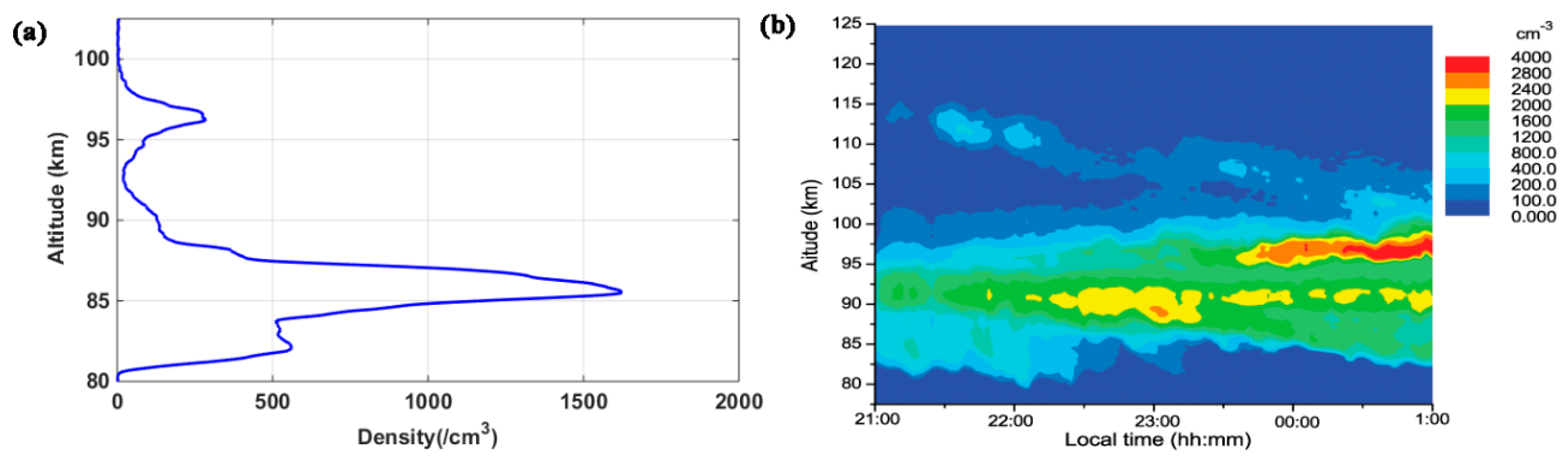
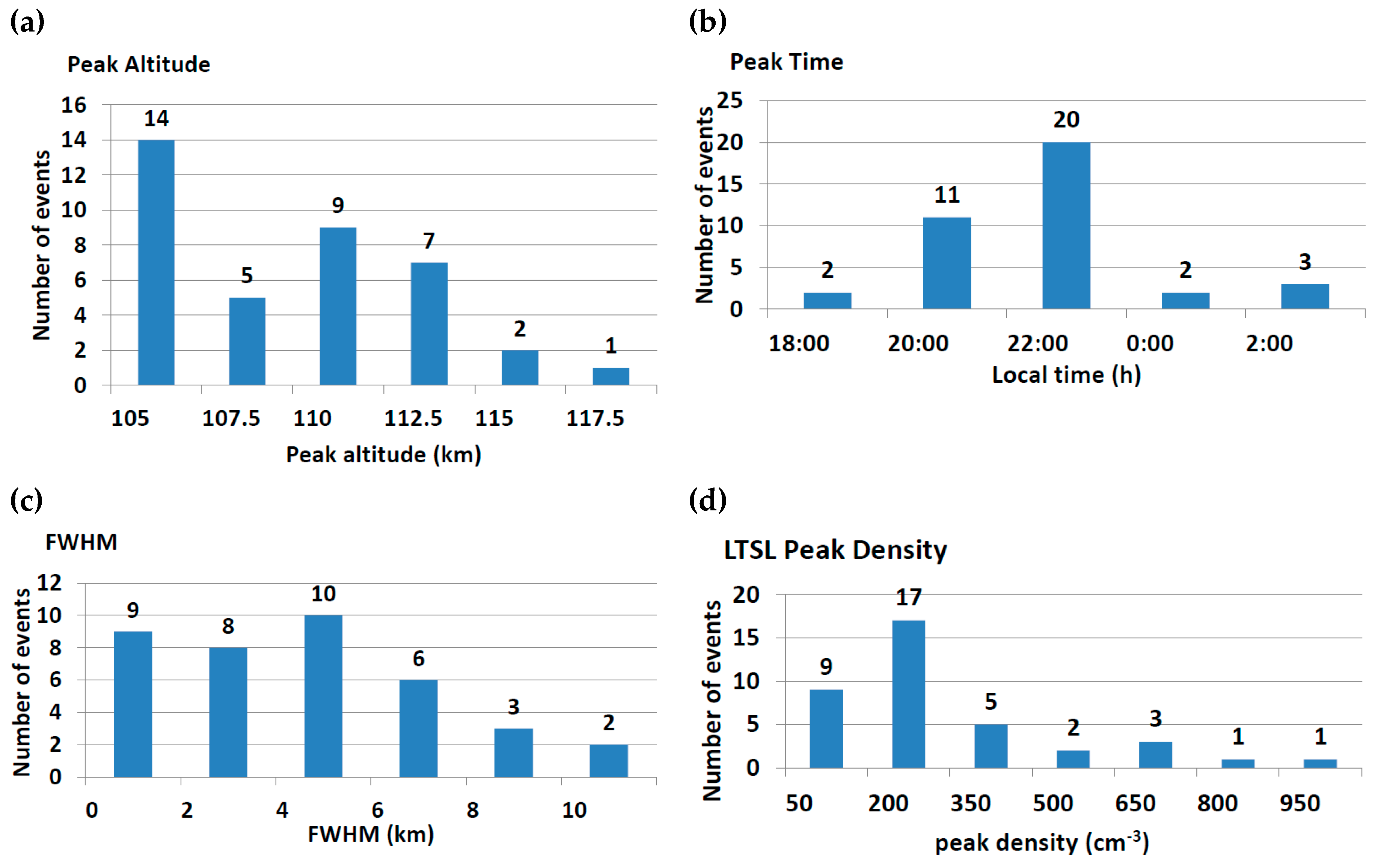
3.1.1. The Parameters of the LTSLs
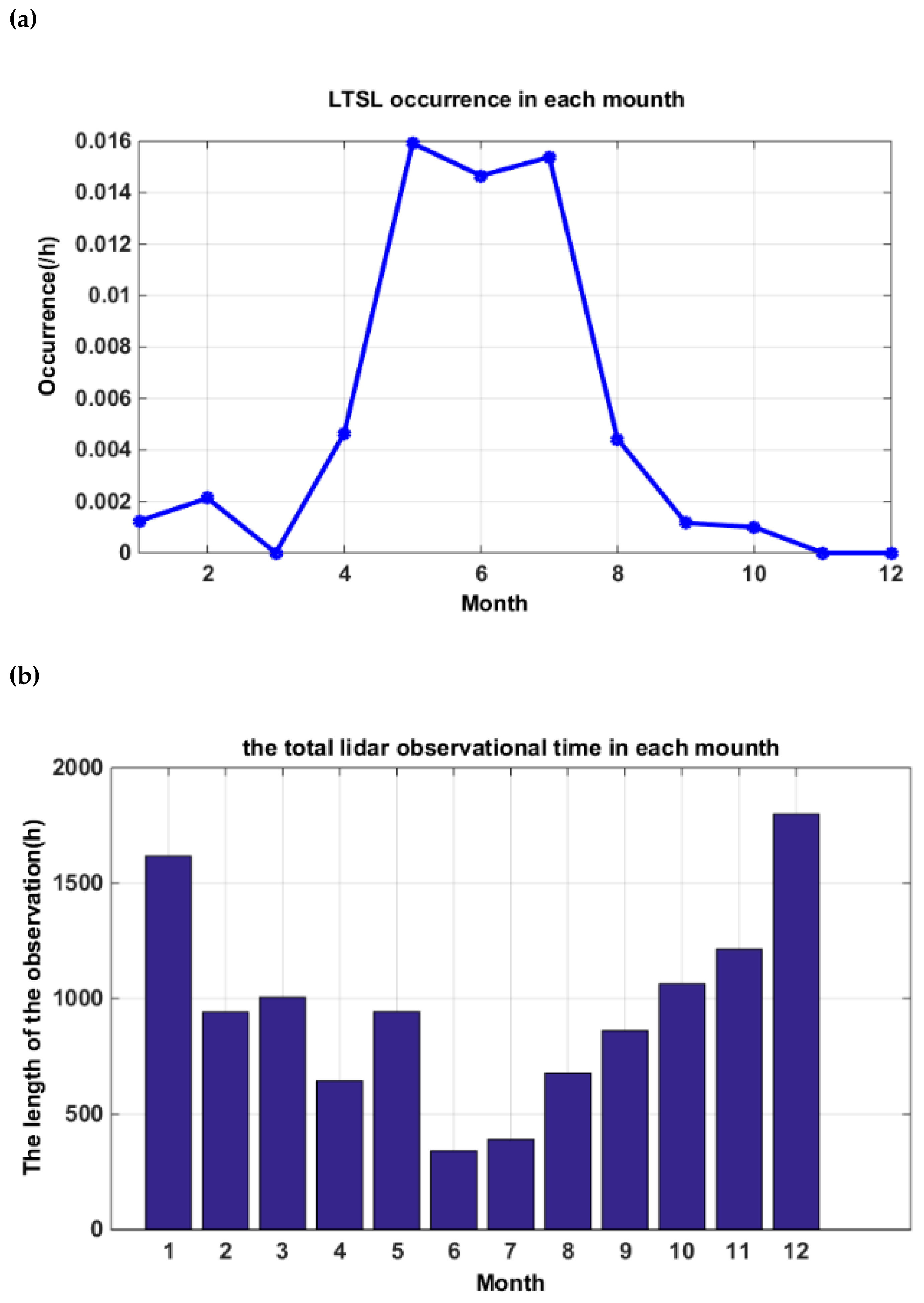
3.1.2. The Seasonal Variations of LTSLs
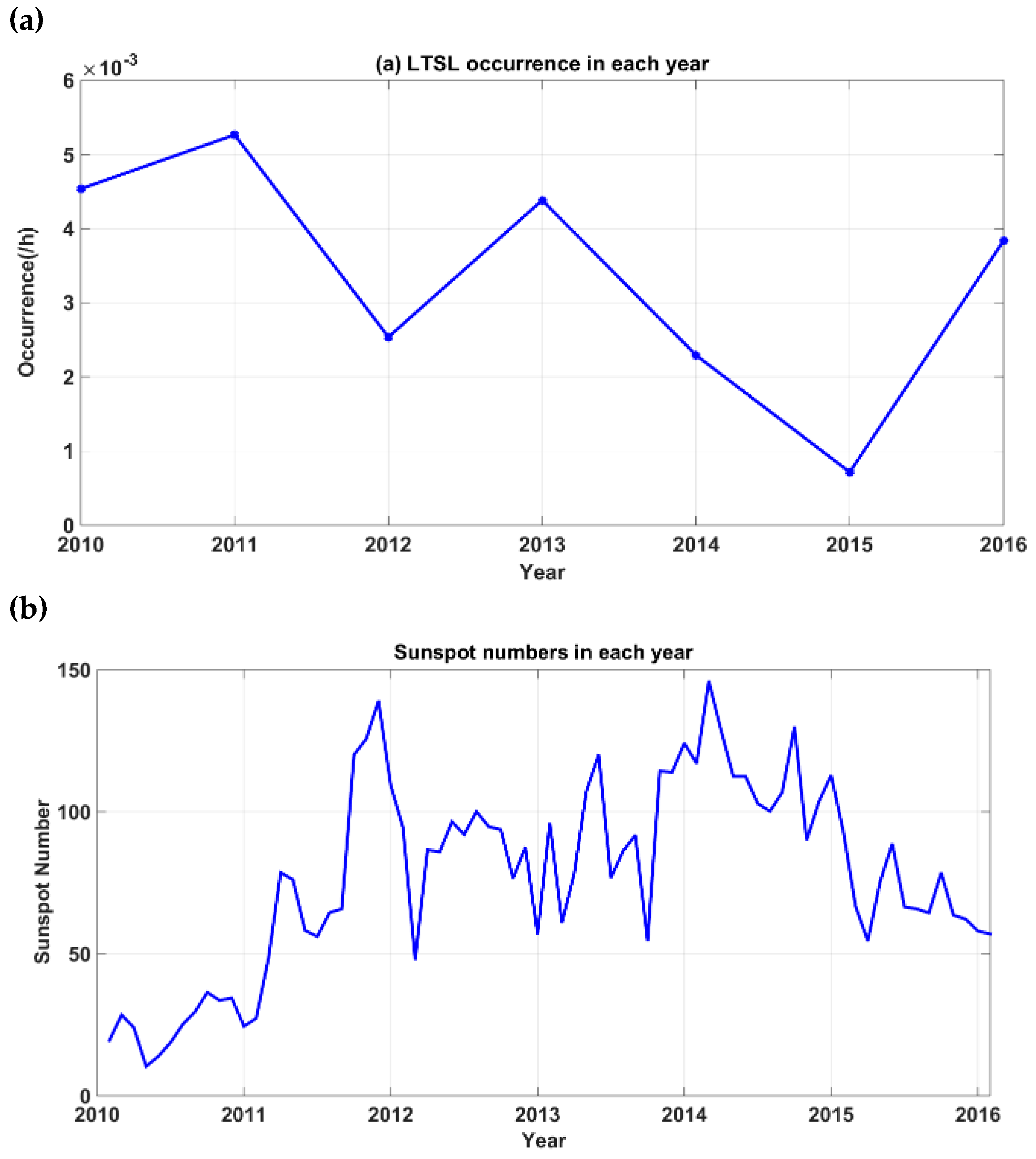
3.1.3. The Inter-Annual Variation of LTSLs
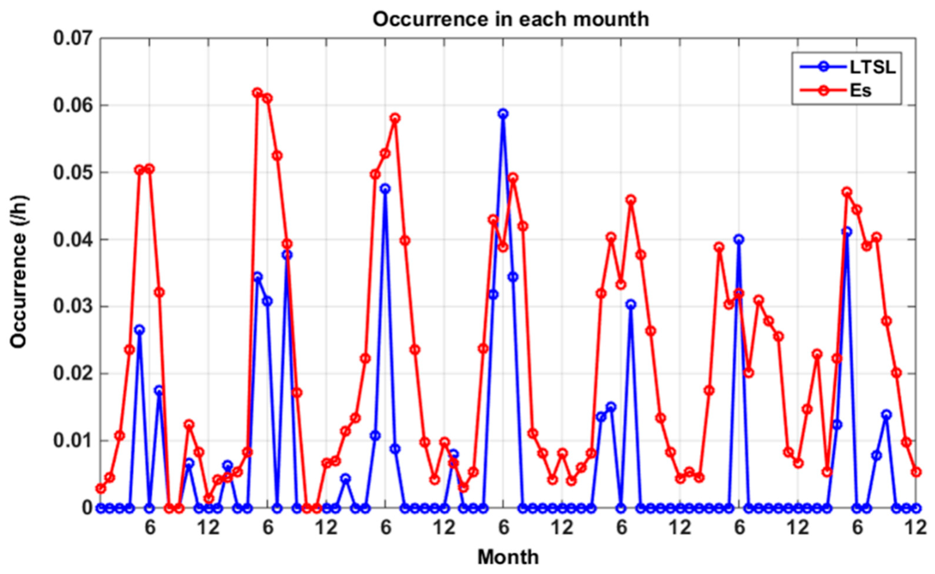
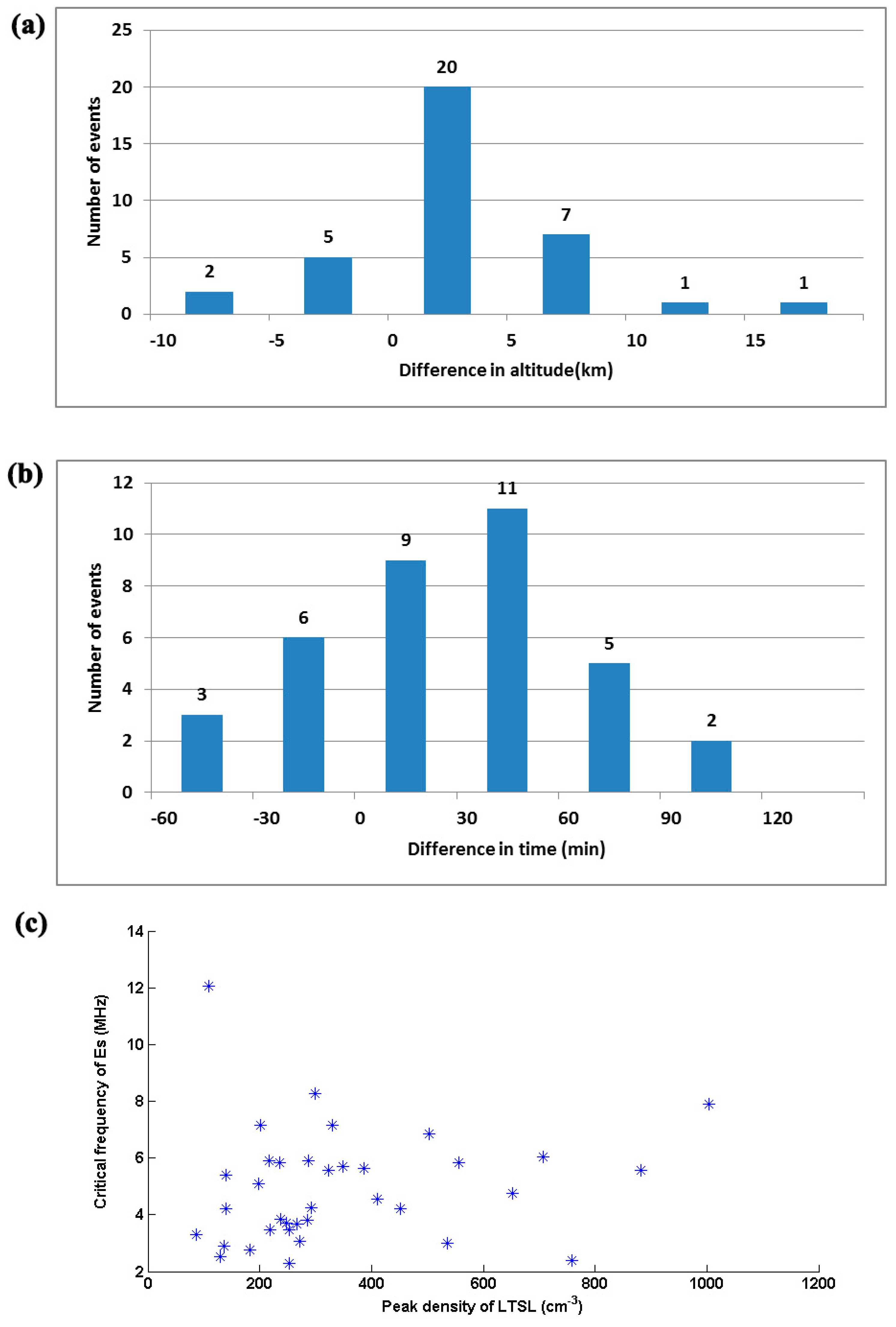
3.2. The Correlation between LTSLs and Es
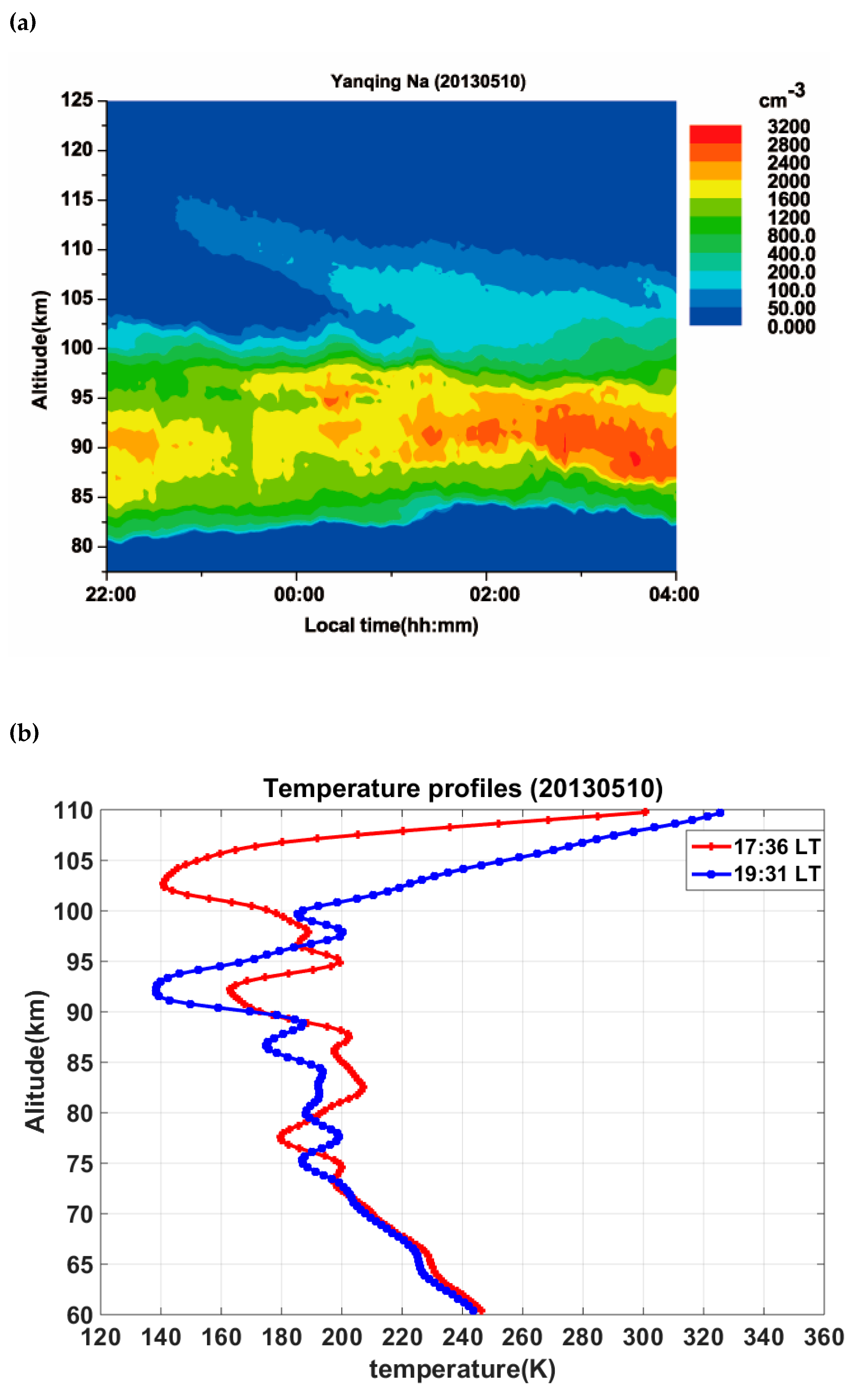
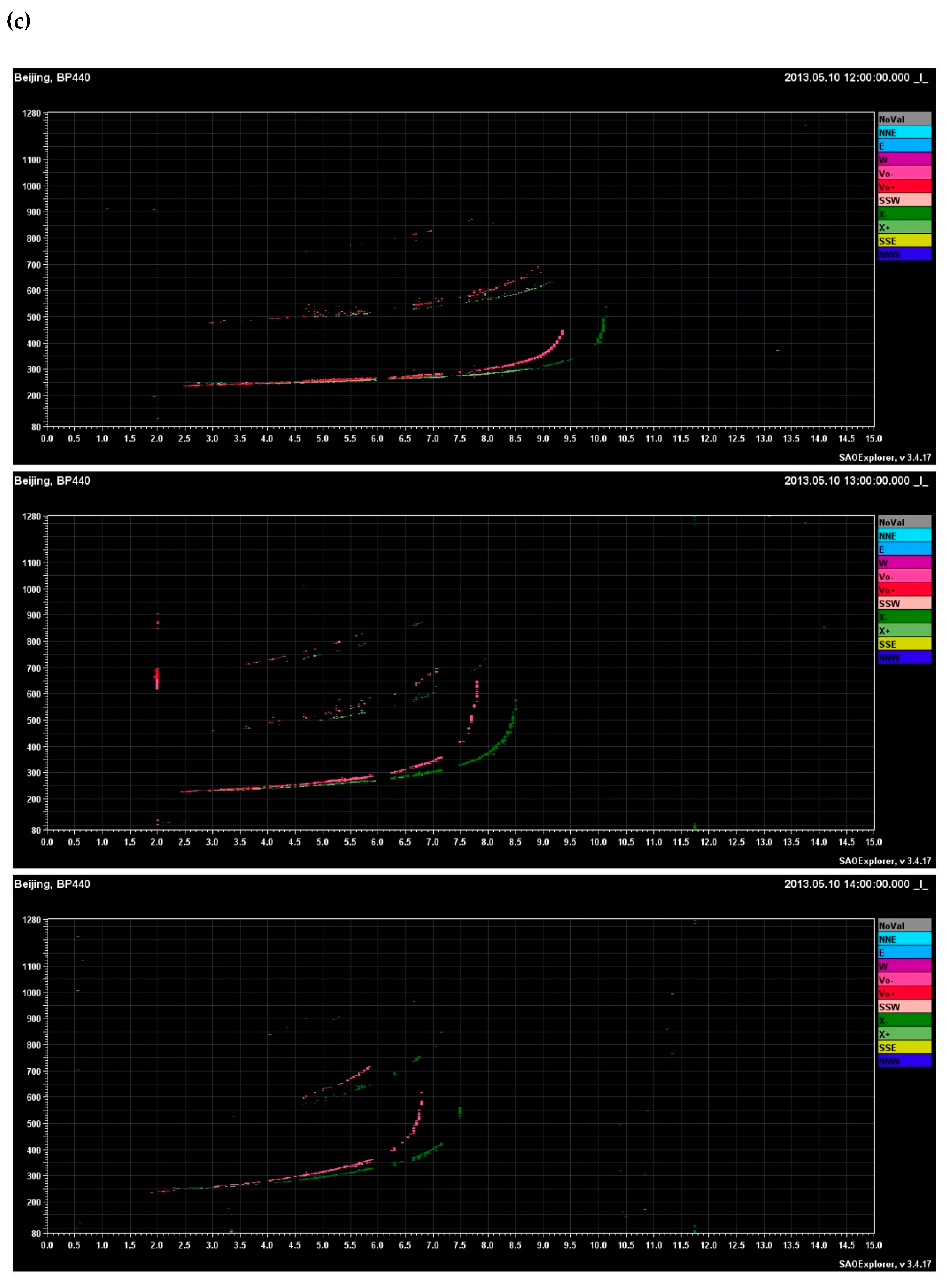
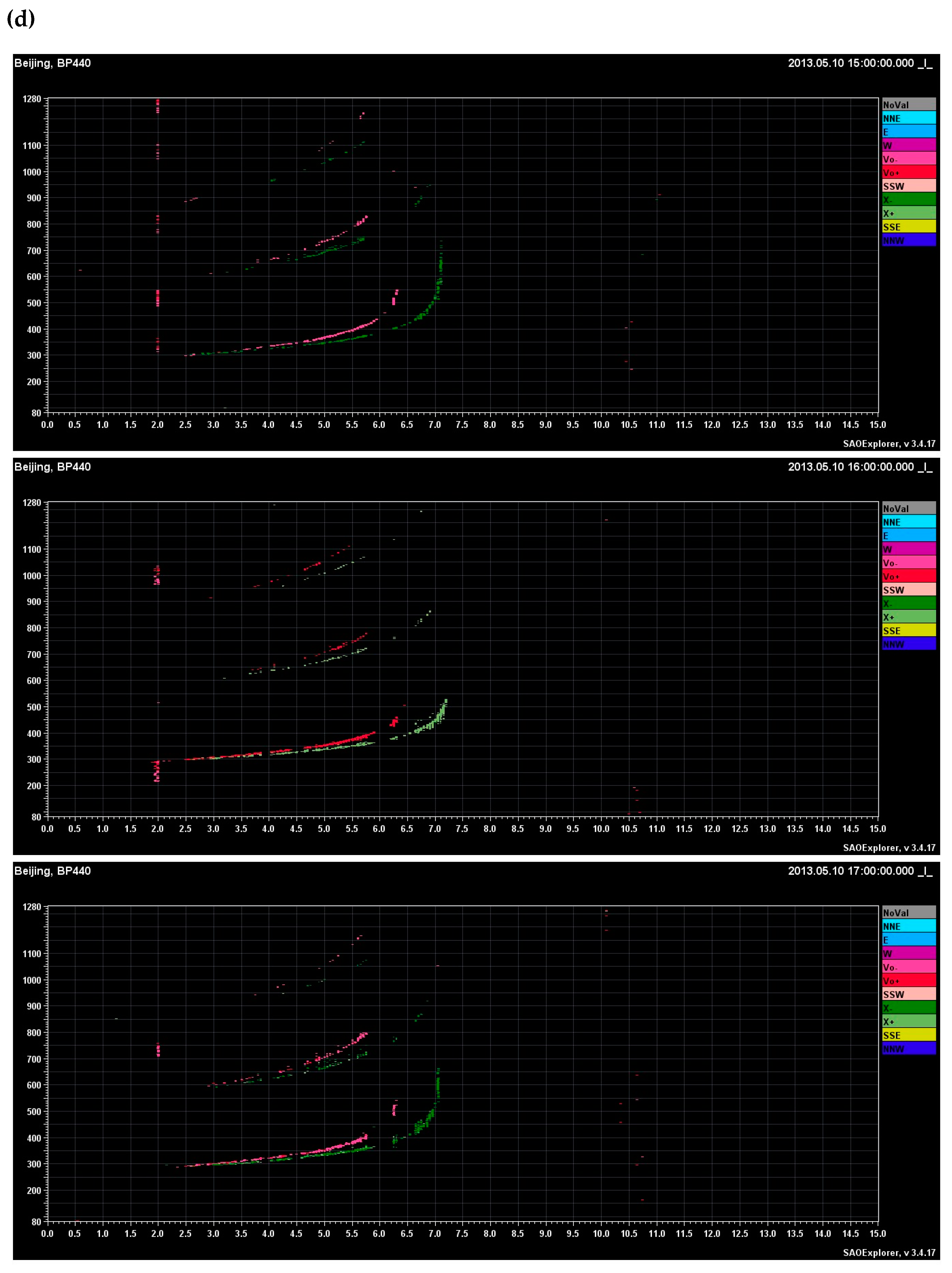
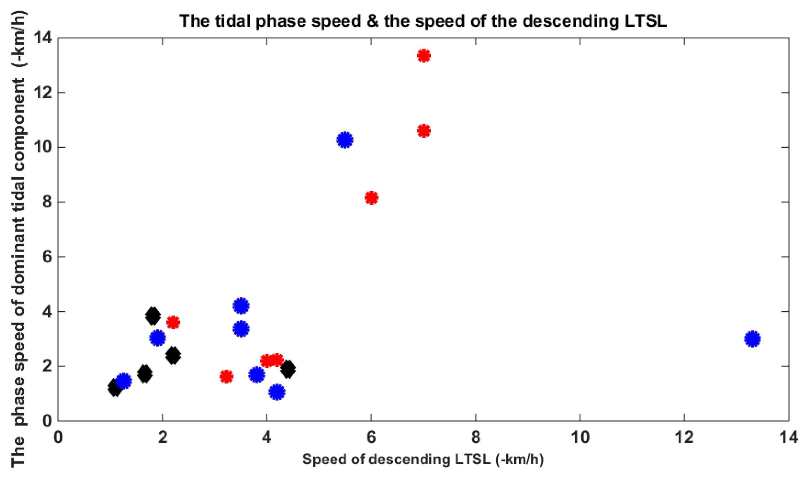
3.3. The Correlation between LTSLs and Tidal Wave
4. Summary
Author Contributions
Funding
Acknowledgments
Conflicts of Interest
References
- Slipher, V.M. Emission in the spectrum of light in the night sky. Publ. Astron. Soc. Pac. 1929, 242, 262–263. [Google Scholar]
- Plane, J.M.; Feng, W.; Dawkins, E.C. The mesosphere and metals: Chemistry and changes. Chem. Rev. 2015, 115, 4497–4541. [Google Scholar] [CrossRef] [PubMed]
- Clemesha, B.R.; Kirchhoff, V.; Simonich, D.; Takahashi, H. Evidence of an extra-terrestrial source for the mesospheric sodium layer. Geophys. Res. Lett. 1978, 5, 873–876. [Google Scholar] [CrossRef]
- Heinselman, C.J.; Thayer, J.P.; Watkins, B.J. A high-latitude observation of sporadic sodium and sporadic E-layer formation. Geophys. Res. Lett. 1998, 25, 3059–3062. [Google Scholar] [CrossRef]
- Fan, Z.Y.; Plane, J.M.C.; Gumbel, J. On the global distribution of sporadic sodium layers. Geophys. Res. Lett. 2007, 34. [Google Scholar] [CrossRef]
- Williams, B.P.; Berkey, F.T.; Sherman, J.; She, C.Y. Coincident extremely large sporadic sodium and sporadic E layers observed in the lower thermosphere over Colorado and Utah. Ann. Geophys. 2007, 25, 3–8. [Google Scholar] [CrossRef][Green Version]
- Simonich, D.; Clemesha, B. Sporadic sodium layers and the average vertical distribution of atmospheric sodium: Comparison of different Nas layer strengths. Adv. Space Res. 2008, 42, 229–233. [Google Scholar] [CrossRef]
- Dou, X.; Xue, X.; Li, T.; Chen, T.; Chen, C.; Qiu, S. Possible relations between meteors, enhanced electron density layers, and sporadic sodium layers. J. Geophys. Res. Space Phys. 2010, 115. [Google Scholar] [CrossRef]
- Tsuda, T.T.; Nozawa, S.; Kawahara, T.D.; Kawabata, T.; Saito, N.; Wada, S.; Hall, C.M.; Oyama, S.; Ogawa, Y.; Suzuki, S.; et al. Fine structure of sporadic sodium layer observed with a sodium lidar at Tromsø, Norway. Geophys. Res. Lett. 2011, 38. [Google Scholar] [CrossRef]
- Takahashi, T.; Nozawa, S.; Tsuda, T.T.; Ogawa, Y.; Saito, N.; Hidemori, T.; Kawahara, T.D.; Hall, C.; Fujiwara, H.; Matuura, N.; et al. A case study on generation mechanisms of a sporadic sodium layer above Tromsø (69.6° N) during a night of high auroral activity. Ann. Geophys. 2015, 33, 941–953. [Google Scholar] [CrossRef]
- Jiao, J.; Yang, G.; Zou, X.; Gong, S.; Wang, J.; Tian, D.; Zhang, W.; Zhang, T.; Yang, X.; Fu, J.; et al. Joint observations of sporadic sodium and sporadic E layers at middle and low latitudes in China. Chin. Sci. Bull. 2014, 59, 3868–3876. [Google Scholar] [CrossRef]
- Nagasawa, C.; Abo, M. Lidar observation of a lot of sporadic sodium layers in mid-latitude. Geophys. Res. Lett. 1995, 22, 263–266. [Google Scholar] [CrossRef]
- Clemesha, B.R.; Batista, P.P.; Simonich, D.M. Formation of sporadic sodium layers. J. Geophys. Res. Space Phys. 1996, 101, 19701–19706. [Google Scholar] [CrossRef]
- Kirkwood, S.; von Zahn, U. On the role of auroral electric fields in the formation of low altitude sporadic-E and sudden sodium layers. J. Atmos. Terr. Phys. 1991, 53, 389–407. [Google Scholar] [CrossRef]
- Cox, R.M.; Plane, J.M.C. An ion-molecule mechanism for the formation of neutral sporadic Na layers. J. Geophys. Res. 1998, 103, 6349–6359. [Google Scholar] [CrossRef]
- Collins, S.C.; Plane, J.M.C.; Kelley, M.C.; Wright, T.G.; Soldán, P.; Kane, T.J. A study of the role of ion–molecule chemistry in the formation of sporadic sodium layers. J. Atmos. Sol. Terr. Phys. 2002, 64, 845–860. [Google Scholar] [CrossRef]
- Collins, S.C.; Hallinan, T.J.; Smith, R.W. Lidar observations of a large high-altitude sporadic Na during active aurora. Geophys. Res. Lett. 1996, 23, 3655–3658. [Google Scholar] [CrossRef]
- Gong, S.; Yang, G.; Wang, J.; Cheng, X.; Li, F.; Wan, W. A double sodium layer event observed over Wuhan, China by lidar. Geophys. Res. Lett. 2003, 30. [Google Scholar] [CrossRef]
- Wang, J.; Yang, Y.; Cheng, X.; Yang, G.; Song, S.; Gong, S. Double sodium layers observation over Beijing, China. Geophys. Res. Lett. 2012, 39, L15801. [Google Scholar] [CrossRef]
- Xue, X.; Dou, X.-K.; Lei, J.; Chen, J.S.; Ding, Z.H.; Li, T.; Gao, Q.; Tang, W.W.; Cheng, X.W.; Wei, K. Lower thermospheric-enhanced sodium layers observed at low latitude and possible formation: Case studies. J. Geophys. Res. Space Phys. 2013, 118, 2409–2418. [Google Scholar] [CrossRef]
- Dou, X.; Qiu, S.; Xue, X.; Chen, T.; Ning, B. Sporadic and thermospheric enhanced sodium layers observed by a lidar chain over China. J. Geophys. Res. Space Phys. 2013, 118, 6627–6643. [Google Scholar] [CrossRef]
- Ma, Z.; Wang, X.; Chen, L.; Wu, J. First report of sporadic Na layers at Qingdao (36° N, 120° E), China. Ann. Geophys. 2014, 32, 739–748. [Google Scholar] [CrossRef][Green Version]
- Tsuda, T.T.; Chu, X.; Nakamura, T.; Ejiri, M.K.; Kawahara, T.D.; Yukimatu, A.S.; Hosokawa, K. A thermospheric Na layer event observed up to 140 km over Syowa Station (69.0° S, 39.6° E) in Antarctica. Geophys. Res. Lett. 2015, 42, 3647–3653. [Google Scholar] [CrossRef]
- Gao, Q.; Chu, X.; Xue, X.; Dou, X.; Chen, T.; Chen, J. Lidar observations of thermospheric Na layers up to 170 km with a descending tidal phase at Lijiang (26.7° N, 100.0° E), China. J. Geophys. Res. Space Phys. 2015, 120, 9213–9220. [Google Scholar] [CrossRef]
- Alan, Z.; Guo, Y.; Vargas, F.; Swenson, G. Firstmeasurement of horizontal wind and temperature in the lower thermosphere (105–140 km) with a Na Lidar at Andes Lidar Observatory. Geophys. Res. Lett. 2016, 43, 2374–2380. [Google Scholar] [CrossRef]
- Xun, Y.; Yang, G.; She, C.-Y.; Wang, J.; Du, L.; Yan, Z.; Yang, Y.; Cheng, X.; Li, F. The first concurrent observations of thermospheric Na layers from two nearby central midlatitude lidar stations. Geophys. Res. Lett. 2019, 46, 1892–1899. [Google Scholar] [CrossRef]
- Chu, X.; Yu, Z.; Gardner, C.S.; Chen, C.; Fong, W. Lidar observations of neutral Fe layers and fast gravity waves in the thermosphere (110–155 km) at McMurdo (77.8° S, 166.7° E), Antarctica. Geophys. Res. Lett. 2011, 38. [Google Scholar] [CrossRef]
- Friedman, J.S.; Chu, X.; Brum, C.G.M.; Lu, X. Observation of a thermospheric descending layer of neutral K over Arecibo. J. Atmos. Sol. Terr. Phys. 2013, 104, 253–259. [Google Scholar] [CrossRef]
- Raizada, S.; Brum, C.M.; Tepley, C.A.; Lautenbach, J.; Friedman, J.S.; Mathews, J.; Djuth, F.T.; Kerr, C. First simultaneous measurements of Na and K thermospheric layers along with TILs from Arecibo. J. Geophys. Res. Space Phys. 2015, 42, 106–112. [Google Scholar] [CrossRef]
- Yuan, T.; Wang, J.; Cai, X.; Sojka, J.; Rice, D.; Oberheide, J.; Criddle, N. Investigation of the seasonal and local time variations of the high-altitude sporadic Na layer (Nas) formation and the associated midlatitude descendingElayer (Es) in lowerEregion. J. Geophys. Res. Space Phys. 2014, 119, 5985–5999. [Google Scholar] [CrossRef]
- Cai, X.; Yuan, T.; Eccles, J.V. A numerical investigation on tidal and gravity wave contributions to the summer time Na variations in the midlatitude E region. J. Geophys. Res. Space Phys. 2017, 122, 10577–10595. [Google Scholar] [CrossRef]
- Cai, X.; Yuan, T.; Pedatella, N.M.; Ban, C.; Liu, A.Z. A Numerical Investigation on the Variation of Sodium ion and observed Thermospheric Sodium Layer at Cerro Pachón, Chile during Equinox. J. Geophys. Res. Space Phys. 2019, 124, 10395–10414. [Google Scholar] [CrossRef]
- Chu, X.; Yu, Z. Formation mechanisms of neutral Fe layers in the thermosphere at Antarctica studied with a thermosphere-ionosphere Fe/Fe+ (TIFe) model. J. Geophys. Res. Space Phys. 2017, 122, 6812–6848. [Google Scholar] [CrossRef]
- Wang, C. Development of the Chinese Meridian Project. Chin. J. Space Sci. 2010, 30, 382–384. [Google Scholar]
- Jiao, J.; Yang, G.; Wang, J.; Cheng, X.; Li, F.; Yang, Y.; Gong, W.; Wang, Z.; Du, L.; Yan, C.; et al. First report of sporadic K layers and comparison with sporadic Na layers at Beijing, China (40.6° N, 116.2° E). J. Geophys. Res. Space Phys. 2015, 120, 5214–5225. [Google Scholar] [CrossRef]
- Wang, Z.; Yang, G.; Wang, J.; Yue, C.; Yang, Y.; Jiao, J.; Du, L.; Cheng, X.; Wang, C. Seasonal variations of meteoric potassium layer over Beijing (40.41°N, 116.01°E). J. Geophys. Res. Space Phys. 2017, 122, 2106–2118. [Google Scholar] [CrossRef]
- Dawkins, E.C.M.; Plane, J.M.C.; Chipperfield, M.P.; Feng, W.; Marsh, D.R.; Höffner, J.; Janches, D. Solar cycle response and long-term trends in the mesospheric metal layers. J. Geophys. Res. Space Phys. 2016, 121, 7153–7165. [Google Scholar] [CrossRef]
- Forbes, J.M.; Zhang, X.; Marsh, D.R. Solar cycle dependence of middle atmosphere temperatures. J. Geophys. Res. Atmos. 2014, 119, 9615–9625. [Google Scholar] [CrossRef]
- Zhou, Q.; Mathews, J.; Tepley, C. A proposed temperature dependent mechanism for the formation of sporadic sodium layers. J. Atmos. Terr. Phys. 1993, 55, 513–521. [Google Scholar] [CrossRef]
- Qiu, S.; Soon, W.; Xue, X.; Li, T.; Wang, W.; Jia, M.; Ban, C.; Fang, X.; Tang, Y.; Dou, X. Sudden sodium layers: Their appearance and disappearance. J. Geophys. Res. Space Phys. 2018, 123, 5102–5118. [Google Scholar] [CrossRef]
- Chimonas, G. Enhancement of sporadic E by horizontal transport within the layer. J. Geophys. Res. 1971, 76, 4578–4586. [Google Scholar] [CrossRef]
- Batista, P.P.; Clemesha, B.R.; Tokumoto, A.S.; Lima, L.M. Structure of the mean winds and tides in the meteor region over Cachoeira Paulista, Brazil (22.7° S, 45° W) and its comparison with models. J. Atmos. Sol. Terr. Phys. 2004, 66, 623–636. [Google Scholar] [CrossRef]


| Date | Peak Time (LT) | Peak Altitude (km) | Peak Density (cm−3) | FWHM (km) | Peak Density of Main Sodium Layer (cm−3) | Ratio |
|---|---|---|---|---|---|---|
| 20100427 | 04:36 | 110 | 130 | 6.8 | 1648 | 7.89% |
| 20100512 | 23:24 | 115 | 247 | 5.4 | 1659 | 14.89% |
| 20100522 | 21:25 | 111 | 1004 | 6.5 | 1707 | 58.82% |
| 20100525 | 22:21 | 115 | 236 | 5.3 | 1505 | 15.68% |
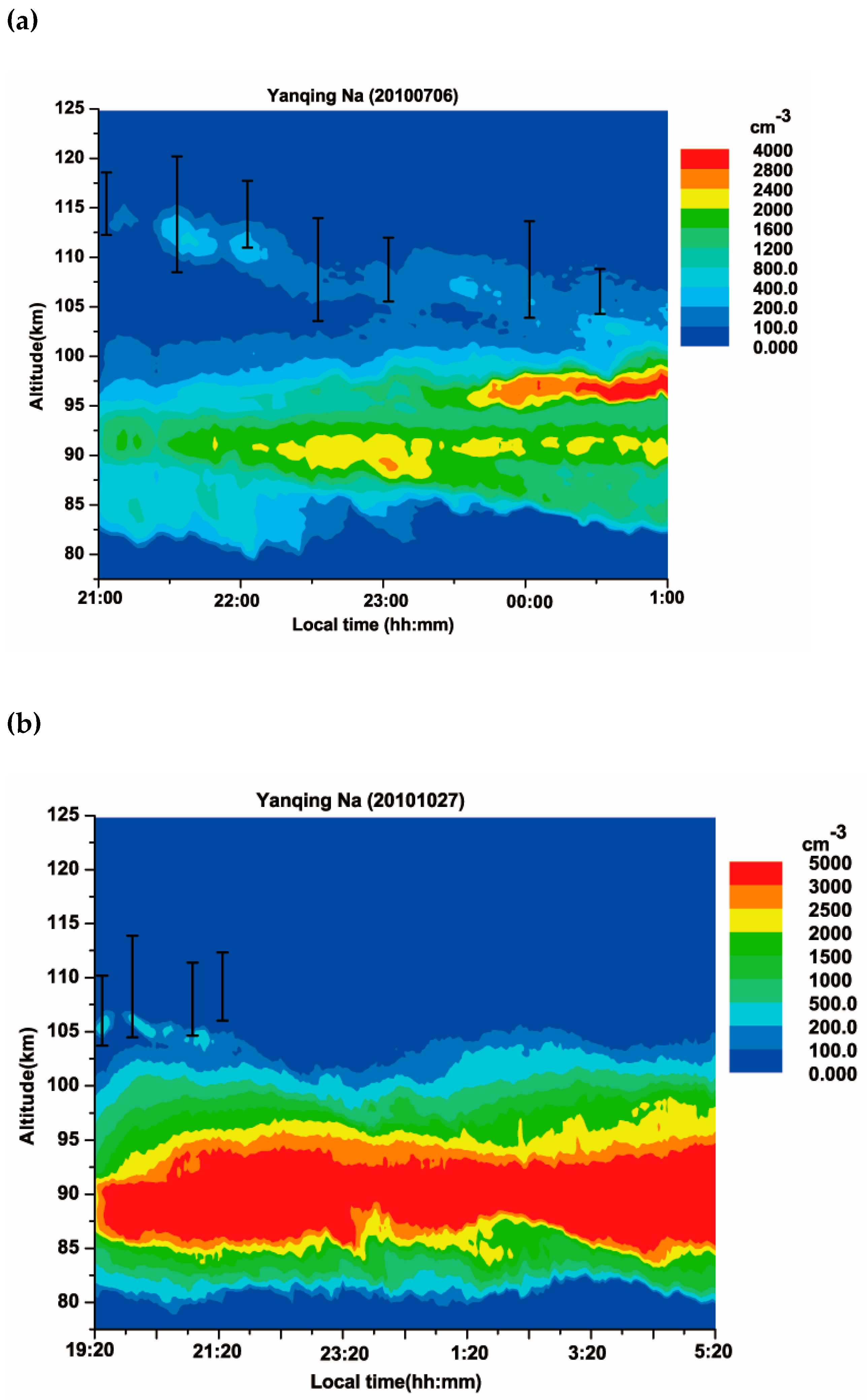
| 20100706 | 21:40 | 112 | 451 | 2.7 | 1706 | 26.44% |
| 20101027 | 19:57 | 106 | 286 | 1.2 | 4202 | 6.81% |
| 20110201 | 22:32 | 105 | 536 | 1.8 | 4889 | 10.96% |
| 20110502 | 22:22 | 110 | 86 | 4.7 | 1700 | 5.06% |
| 20110526 | 20:38 | 113 | 410 | 4.0 | 1656 | 24.76% |
| 20110530 | 22:28 | 113 | 201 | 11.5 | 1366 | 14.71% |
| 20110531 | 22:27 | 105 | 272 | 4.2 | 2087 | 13.03% |
| 20110624 | 23:30 | 110 | 882 | 9.5 | 1666 | 52.94% |
| 20110625 | 21:49 | 110 | 652 | 7.4 | 1670 | 39.04% |
| 20110810 | 22:02 | 105 | 183 | 2.7 | 2723 | 6.72% |
| 20110816 | 22:44 | 106 | 140 | 6.6 | 2591 | 5.40% |
| 20120203 | 23:20 | 105 | 253 | 1.5 | 3552 | 7.12% |
| 20120502 | 23:27 | 115 | 219 | 8.9 | 2923 | 7.49% |
| 20120610 | 23:41 | 115 | 137 | 5.7 | 1644 | 8.34% |
| 20120701 | 21:40 | 118 | 198 | 7 | 2175 | 9.10% |
| 20130116 | 00:12 | 109 | 267 | 3.6 | 5238 | 5.10% |
| 20130117 | 22:51 | 105 | 293 | 4.2 | 5239 | 5.59% |
| 20130510 | 23:42 | 111 | 90 | 5.5 | 1838 | 5.00% |
| 20130519 | 23:10 | 113 | 323 | 3.5 | 2754 | 11.73% |
| 20130611 | 21:38 | 108 | 299 | 4.5 | 2686 | 7.41% |
| 20130705 | 21:21 | 105 | 237 | 1.7 | 1600 | 14.81% |
| 20130716 | 21:17 | 113 | 109 | 5.2 | 1449 | 7.52% |
| 20140430 | 21:06 | 105 | 253 | 1.6 | 4187 | 6.04% |
| 20140504 | 00:23 | 111 | 446 | 6.6 | 3322 | 13.43% |
| 20140525 | 23:51 | 108 | 556 | 3.1 | 3163 | 17.58% |
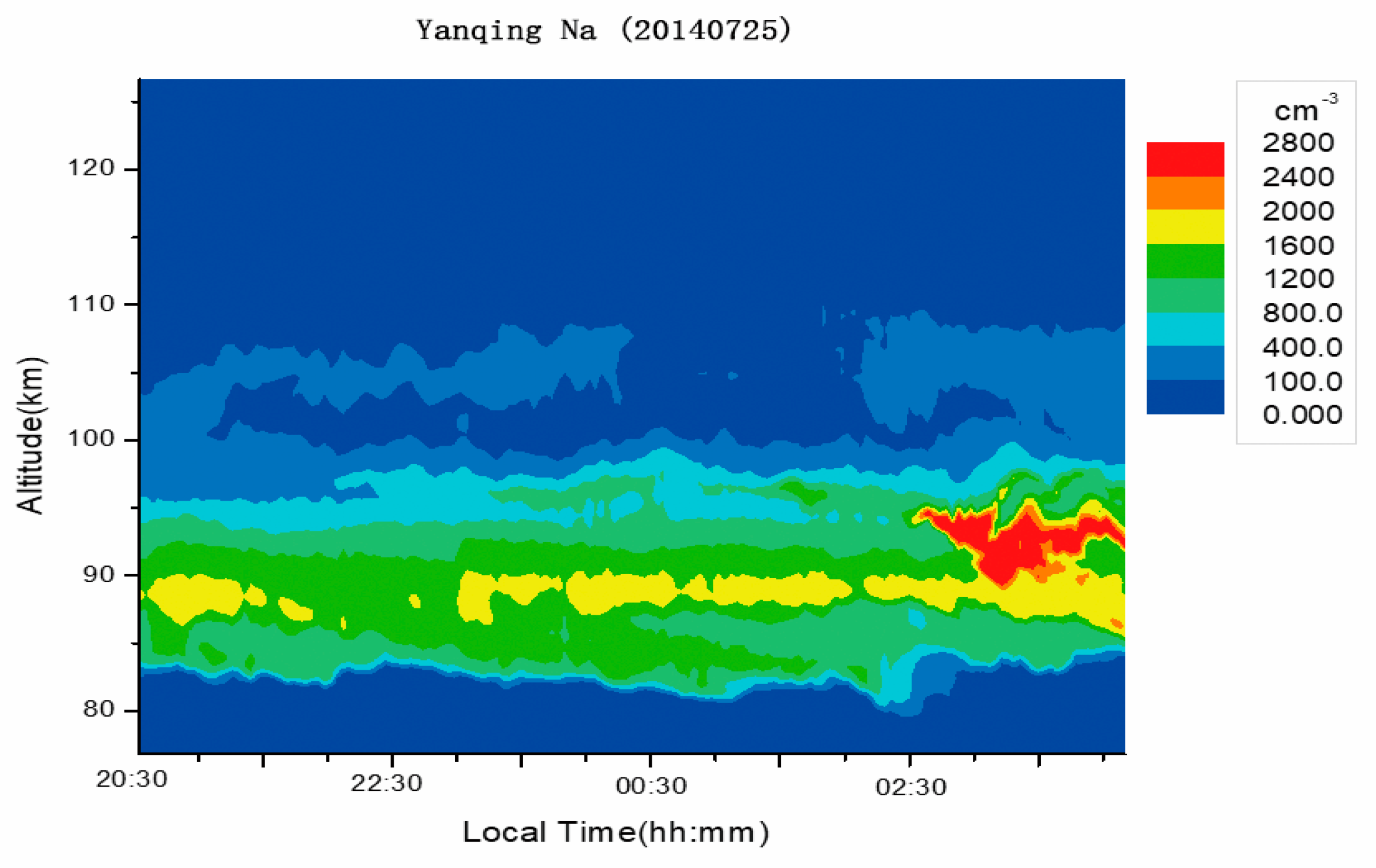
| 20140725 | 22:36 | 106 | 287 | 1.7 | 2211 | 12.98% |
| 20140727 | 21:57 | 106 | 759 | 2.8 | 2873 | 26.00% |
| 20150601 | 22:44 | 110 | 330 | 9.8 | 3380 | 9.76% |
| 20160407 | 02:12 | 107 | 139 | 0.6 | 2502 | 5.56% |
| 20160503 | 23:01 | 110 | 349 | 2.0 | 1831 | 19.06% |
| 20160512 | 02:16 | 113 | 503 | 10.8 | 4519 | 11.13% |
| 20160516 | 20:07 | 108 | 217 | 1.5 | 3004 | 7.22% |
| 20160819 | 22:41 | 105 | 707 | 4.3 | 3405 | 20.76% |
| 20160908 | 19:50 | 106 | 386 | 3.0 | 4375 | 8.82% |
| Data | Beginning of LTSL (LT) | Es Height (km) | Es Time (LT) | Critical Frequency of Es (MHz) |
|---|---|---|---|---|
| 20100427 | 3:34 | 136 | 02:30 | 2.51 |
| 20100512 | 22:59 | 114 | 21:00 | 3.7 |
| 20100522 | 21:22 | 116 | 20:36 | 7.9 |
| 20100525 | 20:52 | 118 | 21:06 | 5.85 |
| 20100706 | 21:26 | 116 | 21:36 | 4.2 |
| 20101027 | 19:20 | 110 | 19:06 | 3.8 |
| 20110201 | 18:22 | 107 | 19:00 | 2.99 |
| 20110502 | 21:42 | 109 | 20:00 | 3.3 |
| 20110526 | 20:38 | 115 | 21:00 | 4.55 |
| 20110530 | 21:40 | 114 | 21:00 | 7.15 |
| 20110531 | 22:27 | 110 | 21:00 | 3.05 |
| 20110624 | 21:48 | 113 | 21:00 | 5.55 |
| 20110625 | 21:14 | 115 | 21:00 | 4.75 |
| 20110810 | 21:07 | 105 | 22:00 | 2.75 |
| 20110816 | 21:29 | 113 | 20:00 | 5.4 |
| 20120203 | 23:20 | 107 | 23:00 | 3.48 |
| 20120502 | 21:39 | 106 | 21:00 | 3.48 |
| 20120610 | 23:18 | 111 | 23:00 | 2.91 |
| 20120701 | 21:40 | 111 | 20:00 | 5.1 |
| 20130116 | 23:02 | 105 | 21:35 | 3.67 |
| 20130117 | 22:51 | 105 | 21:05 | 4.25 |
| 20130510 | 22:41 | None | None | None |
| 20130519 | 21:03 | 113 | 22:00 | 5.55 |
| 20130611 | 21:38 | 113 | 21:00 | 8.27 |
| 20130705 | 20:33 | 120 | 19:05 | 3.85 |
| 20130716 | 20:38 | 112 | 20:00 | 12.07 |
| 20140430 | 20:04 | 113 | 20:00 | 2.3 |
| 20140504 | 22:24 | None | None | None |
| 20140525 | 19:24 | 115 | 18:00 | 5.85 |
| 20140725 | 18:30 | 108 | 18:00 | 5.9 |
| 20140727 | 20:36 | 114 | 20:00 | 2.4 |
| 20150601 | 20:53 | 115 | 21:00 | 7.14 |
| 20160407 | 21:16 | 109 | 20:00 | 4.2 |
| 20160503 | 20:03 | 120 | 20:00 | 5.7 |
| 20160512 | 20:13 | 114 | 20:00 | 6.86 |
| 20160516 | 19:47 | 110 | 19:00 | 5.9 |
| 20160819 | 20:08 | 115 | 20:00 | 6.04 |
| 20160908 | 19:36 | 124 | 20:00 | 5.62 |
| Date | Speed of Descending LTSL (−km/h) | Dominant Tidal Component | Phase Speed of Dominant Tidal Component (−km/h) |
|---|---|---|---|
| 20100427 | - | 24 h | 1 |
| 20100512 | 3.36 | 24 h | 3.5 |
| 20100522 | 1.96 | 8 h | 4.4 |
| 20100525 | 10.59 | 12 h | 7 |
| 20100706 | 3.15 | No data | No data |
| 20101027 | 2.24 | 12 h | 4.2 |
| 20110201 | - | 12 h | 5.25 |
| 20110502 | - | 24 h | 2.34 |
| 20110526 | 1.47 | 24 h | 1.25 |
| 20110530 | 1.71 | 8 h | 1.67 |
| 20110531 | - | - | - |
| 20110624 | - | 12 h | 10 |
| 20110625 | 10.27 | 24 h | 5.5 |
| 20110810 | - | 24 h | 5 |
| 20110816 | 3 | 24 h | 13.3 |
| 20120203 | 1.07 | 24 h | 4.2 |
| 20120502 | 2.19 | 12 h | 4 |
| 20120610 | 1.23 | 8 h | 1.1 |
| 20120701 | 2.31 | - | - |
| 20130116 | 8.14 | 12 h | 6 |
| 20130117 | 1.62 | 12 h | 3.23 |
| 20130510 | 3.6 | 12 h | 2.2 |
| 20130519 | 4.22 | 24 h | 3.5 |
| 20130611 | 1.7 | 24 h | 3.8 |
| 20130705 | - | 24 h | 3 |
| 20130716 | - | 12 h | 5 |
| 20140430 | 13.34 | 12 h | 7 |
| 20140504 | 3.84 | 8 h | 1.82 |
| 20140525 | 3.02 | 24 h | 1.9 |
| 20140725 | - | 6 h | 4 |
| 20140727 | 2.4 | 8 h | 2.2 |
| 20150601 | - | 24 h | 4.67 |
© 2020 by the authors. Licensee MDPI, Basel, Switzerland. This article is an open access article distributed under the terms and conditions of the Creative Commons Attribution (CC BY) license (http://creativecommons.org/licenses/by/4.0/).
Share and Cite
Xun, Y.; Yang, G.; Wang, J.; Du, L.; Wang, Z.; Jiao, J.; Cheng, X.; Li, F.; Zou, X. The Comprehensive Study of Low Thermospheric Sodium Layers during the 24th Solar Cycle. Atmosphere 2020, 11, 284. https://doi.org/10.3390/atmos11030284
Xun Y, Yang G, Wang J, Du L, Wang Z, Jiao J, Cheng X, Li F, Zou X. The Comprehensive Study of Low Thermospheric Sodium Layers during the 24th Solar Cycle. Atmosphere. 2020; 11(3):284. https://doi.org/10.3390/atmos11030284
Chicago/Turabian StyleXun, Yuchang, Guotao Yang, Jihong Wang, Lifang Du, Zelong Wang, Jing Jiao, Xuewu Cheng, Faquan Li, and Xu Zou. 2020. "The Comprehensive Study of Low Thermospheric Sodium Layers during the 24th Solar Cycle" Atmosphere 11, no. 3: 284. https://doi.org/10.3390/atmos11030284
APA StyleXun, Y., Yang, G., Wang, J., Du, L., Wang, Z., Jiao, J., Cheng, X., Li, F., & Zou, X. (2020). The Comprehensive Study of Low Thermospheric Sodium Layers during the 24th Solar Cycle. Atmosphere, 11(3), 284. https://doi.org/10.3390/atmos11030284