Article

Directional Extreme Value Models in Wave Energy Applications

by
Flora Karathanasi
1,2,*,
Takvor Soukissian
2 and
Kostas Belibassakis
1
1
School of Naval Architecture & Marine Engineering, National Technical University of Athens, 15780 Athens, Greece
2
Institute of Oceanography, Hellenic Centre for Marine Research, 19013 Anavyssos, Greece
*
Author to whom correspondence should be addressed.
Atmosphere 2020, 11(3), 274; https://doi.org/10.3390/atmos11030274
Submission received: 28 January 2020 / Revised: 28 February 2020 / Accepted: 7 March 2020 / Published: 10 March 2020
(This article belongs to the Special Issue Waves and Wave Climate Analysis and Modeling)

Abstract

:
A wide range of wave energy applications relies on the accurate estimation of extreme wave conditions, while some of them are frequently affected by directionality. For example, attenuators and terminators are the most common types of wave energy converters whose performance is highly influenced by their orientation with respect to the prevailing wave direction. In this work, four locations in the eastern Mediterranean Sea are selected with relatively high wave energy flux values and extreme wave heights are examined with wave direction as a covariate. The Generalized Pareto distribution is used to model the extreme values of wave height over a pre-defined threshold, with its parameters being expressed as a function of wave direction through Fourier series expansion. In order to be consistent with the analysis obtained from the independent fits for directional sectors, the estimation of parameters is based on a penalized maximum likelihood criterion that ensures a good agreement between the two approaches. The obtained results validate the integration of directionality in extreme value models for the examined locations and design values of significant wave height are provided with respect to direction for the 50- and 100-year return period with bootstrap confidence intervals.

1. Introduction

The design of offshore and marine structures, such as wind turbines and wave energy devices, requires the accurate knowledge of extreme metocean conditions for reliability, viability and safety purposes, since the corresponding variables (e.g., wind speed, significant wave height, current speed) characterize the immediate environment. Most of the relevant studies focus on the estimation of the n—year design values (return levels), for n = 10, 20, …, 100 years, since extreme wave conditions are the most important parameter with respect to safety and reliability of such structures (e.g., Naess [1]; Caires and Sterl [2]; Soukissian and Kalantzi [3]; Caires [4]; Wang [5]). One of the methods that are used for this purpose is the so-called Peaks over Threshold (POT). The POT method is based on the Generalized Pareto (GP) distribution, with which the exceedances of the variable of interest over an appropriately selected high threshold u are modelled under specific assumptions. More details can be found in the reference books of Coles [6] and Leadbetter et al. [7].
The GP distribution [8,9] is a two-parameter distribution, specified by the scale and the shape parameters, σ and ξ, respectively. It has been widely used by many scientists, especially for engineering and environmental studies and hydrology; see, for example, Vanmontfort and Witter [10], Rosbjerg et al. [11], Vogel, et al. [12], Katz, et al. [13], Prudhomme, et al. [14]. The most common methods to estimate the unknown parameters of the GP distribution are the following: (i) the maximum likelihood (ML) method [15]; (ii) the method of moments [16]; (iii) the method of probability weighted moments [17]; (iv) the least squares (LS) method [18]; (v) the elemental percentile method [19] and (vi); the Bayesian technique, proposed by Castellanos and Cabras [20]. Bermudez and Kotz [21] made a review of the above-mentioned estimation methods. The selection of threshold is critical for the accurate estimation of the parameters of the GP distribution and in turn, return levels. When the threshold value is reduced, the asymptotic arguments, which are important when selecting an extreme value distribution, might be invalid. On the other hand, a high enough threshold may lead to high variance of the estimator by reducing the sample size. However, since there is not a generally accepted method for the selection of the most appropriate threshold, a plethora of methods can be applied for threshold selection; see the recent reviews of Scarrott and MacDonald [22] and Langousis et al. [23] on this issue. One of the main categories for threshold selection belong to the graphical methods (e.g., Drees, et al. [24]), while methods based on the goodness-of-fit of the GP distribution are also popular (e.g., Choulakian and Stephens [25]; Northrop and Coleman [26]), for which the lowest threshold is selected so that the corresponding exceedances can adequately described by the GP distribution.
Another issue that needs attention is the validity of the independence assumption as regards the exceedances. The POT method assumes that exceedances are mutually independent and identically distributed. However, threshold exceedances of significant wave height Hs tend to occur in groups with a strong correlation of wave conditions in time, hence violating the assumption of independence. In order to ensure that the threshold exceedances are approximately independent so that they can be used to apply the GP distribution model, declustering of exceedances takes place; see, for example, Leadbetter, et al. [7]. This technique stipulates that the exceedances that are separated by fewer than r non-exceeding observations, with r an auxiliary parameter denoting the run length (minimum separation), form a single cluster. Then, the GP fitting is performed only for the largest exceedances from each cluster instead of all the observations exceeding the threshold.
In the context of ocean energy technology and monitoring systems (e.g., oceanographic buoys), the knowledge about the extreme behavior of wind and wave characteristics including directional dependence is crucial. For instance, most of the support structures for offshore wind turbines, either fixed or floating, are non-axisymmetric (apart from monopile foundations) leading to different operational response and capacity as regards loading intensity from metocean characteristics and fatigue performance. Analogously, there are wave energy converters (WECs), deployed either offshore or nearshore, whose performance is highly affected by their orientation with respect to the prevailing sea state direction. Specifically, attenuators are elongated floating devices that are oriented parallel to the wave direction, with a horizontal extent comparable to the wavelength, while terminators are oriented perpendicular to the predominant wave direction. The fact that the overall cost of energy can be lowered through the continuous development of design of such structures and improved risk assessment techniques render directionality an integral part of design optimization, reliability and safety maximization. On top of that, current regulations and standards from well-established organizations related to engineering design principles for structures at sea, such as the American Bureau of Shipping (ABS) and the Det Norske Veritas (DNV), recommend as well the consideration of directionality to ensure proper structural safety; see, for example, ABS [27] and DNV [28].
At a given location the long-term variability of a parameter under investigation depends inter alia on the component of direction. For instance, extreme values of Hs are usually observed for specific directional sectors depending on the particular characteristics of the location examined (e.g., fetch length, bathymetry). In the context of describing the extremal properties of wave parameters, it is common practice to work with hindcast data sets beside the fact that wave measurements are limited in time (and in space) rendering them inappropriate for extrapolation purposes. Hindcast products have the full information as regards wave conditions, hence mean wave direction can be taken into account and treated as a covariate in order to obtain an integrated and more accurate model for the estimation of the corresponding design values. The significance of directional behavior in works related to offshore/coastal structures for harvesting marine resources has been highlighted by many authors; see, for example, Soukissian [29]; Wei et al. [30]; Soukissian and Karathanasi [31]. Nevertheless, the involvement of directionality, along with other covariates such as space, in extreme value analysis has gained ground mainly the past 15 years, with some sporadic works in the meantime dating back to the early 80′s.
Specifically, Moriarty and Templeton [32] estimated extreme wind gusts for six directional sectors by fitting a Generalized Extreme Value distribution in the design of large buildings. Maximum wind speed as a function of direction has also been modelled by Coles and Walshaw [33], considering a dependence structure across directions, because their a priori division leads to correlated directional sectors and adapting techniques developed for spatial extremes. Similar approaches for modelling extreme wind speed with a directional dependence structure have been presented by for example, Simiu et al. [34] and Solari and Losada [35]. A methodology for the appropriate selection of uncorrelated directional sectors has been proposed by Folgueras et al. [36], which reduces also the uncertainty in the estimation of design values of wind speed. Sea currents have been investigated in the work of Robinson and Tawn [37] by means of a parametric model for extreme current data by handling not only directionality but temporal dependence and non-stationarity as well.
In a series of papers, Ewans and Jonathan [38], Ewans and Jonathan [39], Jonathan and Ewans [40] and Jonathan et al. [41] have highlighted the importance of including directionality and seasonality when studying extreme wave design criteria especially in storm-dominated regions. In the above studies, extreme value modelling of storm peak significant wave height was based on GP distribution with its unknown parameters expressed as a function of direction, while a risk-cost approach was proposed for the construction of directional design criteria.
A common approach for the estimation of the design values is to bin the Hs values above the defined threshold into directional sectors (either fixed or arbitrarily), perform extreme analysis in each sector and then specify design values for a given return period for each sector. However, as stated explicitly by Forristall [42], this sectoring approach leads to inconsistencies with the omni-directional case in terms of design values while it is insufficient at locations where directionality is limited to specific directional sectors. Following the rationale proposed by Robinson and Tawn [37] and Jonathan and Ewans [40], the directional effects vary smoothly so that wave data and their actual behavior in the marine environment are better represented by means of a smooth periodic function.
One of the objectives of this paper is to propose a penalized likelihood criterion for the estimation of the unknown parameters of the directional extreme value model, which seems to be numerically stable for optimization. The unknown parameters are expressed by means of a Fourier series expansion and even for higher-order expressions the solution seems to be stable, when the penalty term is considered. Moreover, a thorough analysis is performed as regards the methods of threshold selection and declustering in order to obtain a better understanding of the effects of the different combinations on the estimation of the GP parameters and the design values of Hs taking into account directionality effects. In this context, three methods as regards threshold selection that are widely used in the relevant literature are examined, namely mean excess function, threshold stability and percentiles, along with two common declustering methods, that is, intervals and runs declustering methods. An additional method for declustering extreme data proposed by Soukissian and Kalantzi [43] is also assessed.
The paper is structured as follows. In Section 2, the parameters of the GP distribution are expressed through the standard directional extreme value model and a synopsis for the estimation parameters using ML is presented. The inclusion of a penalty term in ML is also proposed in order to obtain a more stable and reliable solution in the estimation of parameters. Moreover, an outline for the estimation of the Hs design values is provided. The key features of the most frequently used threshold selection and declustering methods are briefly described along with the DeCA declustering method, which is physically consistent with the wave phenomenon. Section 3 deals with the estimation of the uncertainties of parameters and design values focusing on the bias-corrected and accelerated bootstrap method. In Section 4, the hindcast wave data are presented and statistically analyzed, with respect to Hs and mean sea state direction θw, for four locations in the eastern Mediterranean Sea. Section 5 includes some preliminary results regarding the determination of the proposed directional model by considering all the combinations of the methods presented in Section 2, while the final results of parameter estimates and design values along with their uncertainties is presented for a particular combination (based on the maximum number of exceedances) for all locations. The last section includes the concluding remarks of this analysis and suggestions for further research directions.

2. Directional Extreme Value Model

Let assume that there is a linear random variable X and a corresponding sample { x i } i = 1 n , along with the sample { θ i } i = 1 n for the associated directional random variable, say Θ . Assuming that the GP distribution describes the extreme observations above a threshold u , which is considered independent of the directional variable Θ , the cumulative distribution function (cdf) of Y j = X ( j ) u , j = 1 , , n u , with X ( j ) denoting the observations that exceed the threshold u , is given by
G Y j | θ j . u ( y ; σ u , ξ ) = 1 ( 1 + ξ ( θ j ) y σ u ( θ j ) ) 1 / ξ ( θ j ) , y > 0 ;   σ u > 0 ,
for 1 + ξ ( θ j ) y / σ u ( θ j ) > 0 , where ξ is the shape parameter and σ u > 0 is the scale parameter, both expressed as functions of θ j , with { θ j } j = 1 n u .
In the context of estimating the unknown parameters, as noted by Robinson and Tawn [37], it is expected that they vary smoothly with direction. Thus, a Fourier series expansion is used for the description of this (angular) dependence, which assures a periodic behavior of the estimates in terms of the direction. In this respect, the general form of the Fourier series is for ξ and σ u
k = 0 p b = 1 2 A b k t b ( k θ )   and   k = 0 p b = 1 2 B b k t b ( k θ ) ,
respectively, where p denotes the order of the Fourier model, t 1 , t 2 is the cosine and sine function, respectively. A b k , B b k are the unknown parameters for ξ and σ u , respectively. For example, the first order Fourier model results in the following relationships:
ξ ( θ ) = A 10 + A 11 cos ( θ ) + A 21 sin ( θ )   and   σ ( θ ) = B 10 + B 11 cos ( θ ) + B 21 sin ( θ ) .
As noted by Jonathan and Ewans [40], the proper order of the model is determined by the directional dependence of the data sample in hand; the more complex the directional dependence that characterize the data, the higher the model order is.

2.1. Parameter Estimation

The unknown parameters A b k and B b k , b = 1 ,   2 , k = 0 , ,   p , are estimated by applying ML estimation. The likelihood of the corresponding data sample { Y j } j = 1 n u is obtained by
L ( { A b k } , { B b k } ; { Y j } j = 1 n u ) = j = 1 n u 1 σ u ( θ j ) ( 1 + ξ ( θ j ) σ u ( θ j ) Y j ) ( 1 / ξ ( θ j ) ) 1 ,
and the negative log-likelihood (for ξ ( θ j ) 0 ) by
= i = 1 n u [ log σ u ( θ i ) + ( 1 + 1 ξ ( θ i ) ) log ( 1 + ξ ( θ i ) σ u ( θ i ) Y i ) ] .
ML estimates can be determined by setting the partial derivatives of with respect to A b k and B b k , b = 1 ,   2 , k = 0 , , p , equal to zero, that is:
A b k = j = 1 n u { [ 1 [ ξ ( θ j ) ] 2 ( log ( 1 + ξ ( θ j ) σ u ( θ j ) Y j ) ( 1 + ξ ( θ j ) ) ( ξ ( θ j ) Y j σ u ( θ j ) + ξ ( θ j ) Y j ) ) ] t b ( k θ j ) } = 0
and
B b k = j = 1 n u { 1 σ u ( θ j ) [ σ u ( θ j ) Y j σ u ( θ j ) + ξ ( θ j ) Y j ] t b ( k θ j ) } = 0 ,
respectively. For large samples, the restriction for the ML estimator for the GP distribution to ensure consistency, asymptotical normality and asymptotical efficiency is that ξ > 0.5 , referred to as the regular case [16]. For ξ 0.5 , we have the non-regular case and for ξ > 1 , ML estimators do not exist.
In this work, a penalty criterion is recommended for the extreme value estimates to ensure that the directional dependence of ξ and σ u is sufficiently described and that the solution is stable even if either the order of the Fourier model is high or the weighting constant of the penalty term is small, as is presented in Section 5. This penalty term is based on the absolute difference between the estimates and the initial values of the parameters obtained from the independent fits calculated using data from successive directional sectors of, say, 45-degree width so that ξ ( θ ) and σ u ( θ ) are consistent with ξ and σ u obtained from the independent fits of each directional sector. As discussed in Section 5, the minimum number of the 45-degree width sectors with sufficient amount of data should be set. This number depends on the order of the Fourier model, along with the amount of data of each sector per se. With the inclusion of the penalty term in the model fitting, the terms that are not consistent are penalized appropriately. In this case, the negative log-likelihood with the penalty term takes the form
P = + w i = 1 2 ( 1 + 2 p ) | ϑ i ϑ ^ i | ,
where w is a constant that gives the appropriate weight for the penalty term in model fitting and ϑ i , ϑ ^ i denote the initial and final values of the unknown parameters, respectively, with p indicating the order of the model. In Ewans and Jonathan [39], a roughness penalty, selected using the cross-validation criterion, was adopted in order to obtain as smooth as possible estimates. In Figure 1, a preliminary result is presented for a particular location (further analyzed in Section 4 and Section 5), which shows the instability of a high order Fourier model. The solid lines denote the form of the estimated parameters ξ and σ u obtained from the standard ML and the dashed lines denote the penalized version of ML with w = 1 . This result clearly shows the instability of the standard ML method when the order of the Fourier model is high. For this particular order, the Fourier model has a better fit compared with the independent fits with data from eight consecutive sectors of 45-degree width, while the standard directional model shows a rather oscillatory behavior with a poor performance.
The directional extreme value model can be determined if the order of the model p is specified and the constant w is selected. In order to justify whether the inclusion of the directional covariates into the model is significant and judge which order of the Fourier model is the most adaptable in terms of capturing directional dependence, the likelihood-ratio (LR) test can be applied [6,44]. This test is widely used when nested models are compared. Suppose that the basic model M 0 is nested within model M 1 , which is more complex (e.g., the zeroth- and first-order directional models, respectively) with values of the negative log-likelihood 0 and 1 , respectively. The LR test statistic is then expressed as
T LR = 2 ( 0 ( M 0 ) 1 ( M 1 ) ) .
Under the null hypothesis that model M 0 is the true model, the distribution of T LR is evaluated by assessing whether the additional complexity of model M 1 leads to a better improvement in terms of performance compared to model M 0 . The asymptotic distribution of T LR under the null model is a χ k 2 distribution with k denoting the degrees of freedom equal to the difference among the number of the models parameters. As long as the sample size is reasonably large, it is common to assume that this distribution is valid for finite samples as well. Consequently, the null hypothesis is rejected at the α level of significance if T LR exceeds the ( 1 α ) quantile of the χ k 2 distribution. Hence, model M 1 is selected in favour of model M 0 .
Given the order of the Fourier model for ξ ( θ ) and σ u ( θ ) , the constant w has to be set. This selection is based on the minimization of the distance between the values of the estimated parameters ξ and σ u from the independent fits and the corresponding ones from the directional model. The statistical metric that was selected due to the fair treatment of positive and negative differences is the mean absolute error that is defined as follows:
MAE = 1 N S i = 1 p | ϑ ^ i ϑ i | ,
where ϑ denotes the parameters ξ and σ u estimated from the independent fits, ϑ ^ the corresponding parameters estimated from the directional model and N S is the number of directional sectors. The optimum value for w is selected when the metric is minimized for both parameters simultaneously.

2.2. Design Values for Directional Extreme model

Supposing that the GP distribution is suitable for modelling the exceedances and having estimated its unknown parameters by the proposed method, we easily obtain the following result
P [ X > x ] = p u [ 1 + ξ ^ ( θ ) ( x u σ ^ u ( θ ) ) ] 1 / ξ ^ ( θ ) ,
where p u = P [ X > u ] , that is, the probability of threshold exceedance. Introducing the term ‘mean exceedance rate,’ which is the average number of observations above the threshold u per year, an estimate of p u can be given by the empirical distribution function
p ^ u = n u n ,
where n u is the number of observations exceeding the threshold u . Let it be noted that p ^ u is also the ML estimate of p u , since the number of threshold exceedances follow the binomial distribution B i n ( n , p u ) .
Now, assuming that n measurements X 1 , , X n were taken during n y observation years then it is implied that during T years there are n T / n y observations. Thus, the x T return level (that is exceeded on average once in T years) is obtained by rearranging Equation (8) and using Equation (9). The return level (design value) x T for a given return period T can be estimated by
x T = { u + σ ^ u ( θ ) ξ ^ ( θ ) [ ( n u T n y ) ξ ^ ( θ ) 1 ] ,           ξ ^ ( θ ) 0 u + σ ^ u ( θ ) l n ( n u T n y ) ,      ξ ^ ( θ ) = 0 ,

2.3. Methods for Threshold Selection

The a priori selection of a suitable threshold implies the existence of an additional unknown parameter for the GP distribution, which may affect the validity of the estimates and is still an open issue with no established commonly accepted approach. This selection is a trade-off between bias and variance. A low threshold will result in large bias and low variance leading to incorrect results for the obtained estimates since less representative extreme data are taken into account whereas a high threshold will result in small bias and large variance in the estimation of the parameters, leading to unreliable results due to the smaller sample size.
A plethora of statistical techniques has been proposed for the determination of the appropriate threshold. According to the work of Langousis et al. [23], these methods can be roughly categorized as follows: (i) graphical methods where one searches for linear behavior of the GP parameters (or related metrics) within a range of thresholds, such as mean residual life plot and parameter stability plot; (ii) goodness-of-fit-tests that detect the lowest threshold for which the GP distribution is suitable either by minimizing the asymptotic mean square error of the estimators or quantifying the deviations between the theoretical distribution and the empirical cdf, and; (iii) non-parametric methods that determine the appropriate starting point of the extreme region of the data record. Since each method leads to different threshold choices, the sensitivity of the inferences (as regards parameter estimation) is evaluated as well. Thus, in the subsequent sections, a summary of the most widely used approaches that will be used in this work is presented.

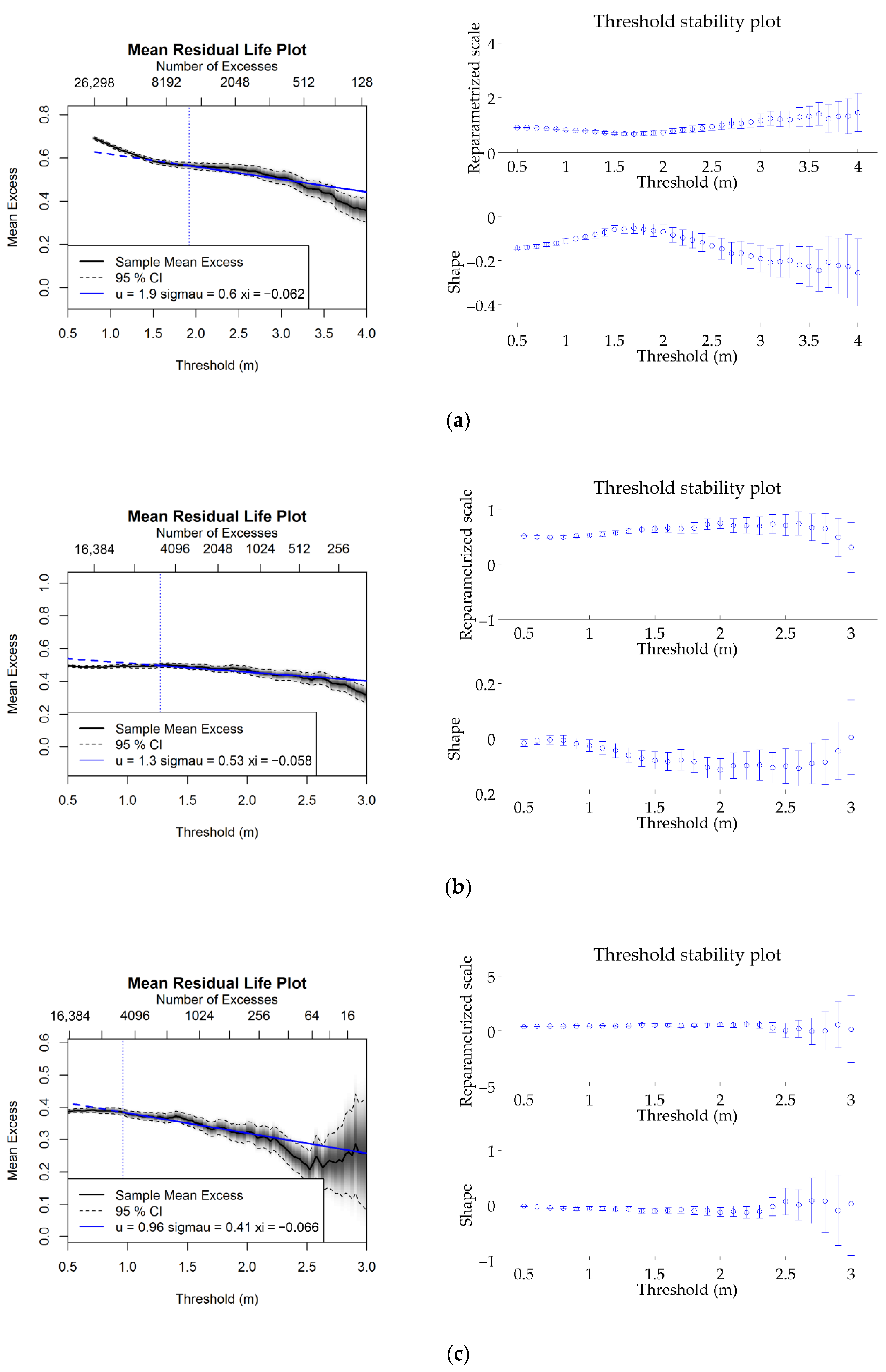
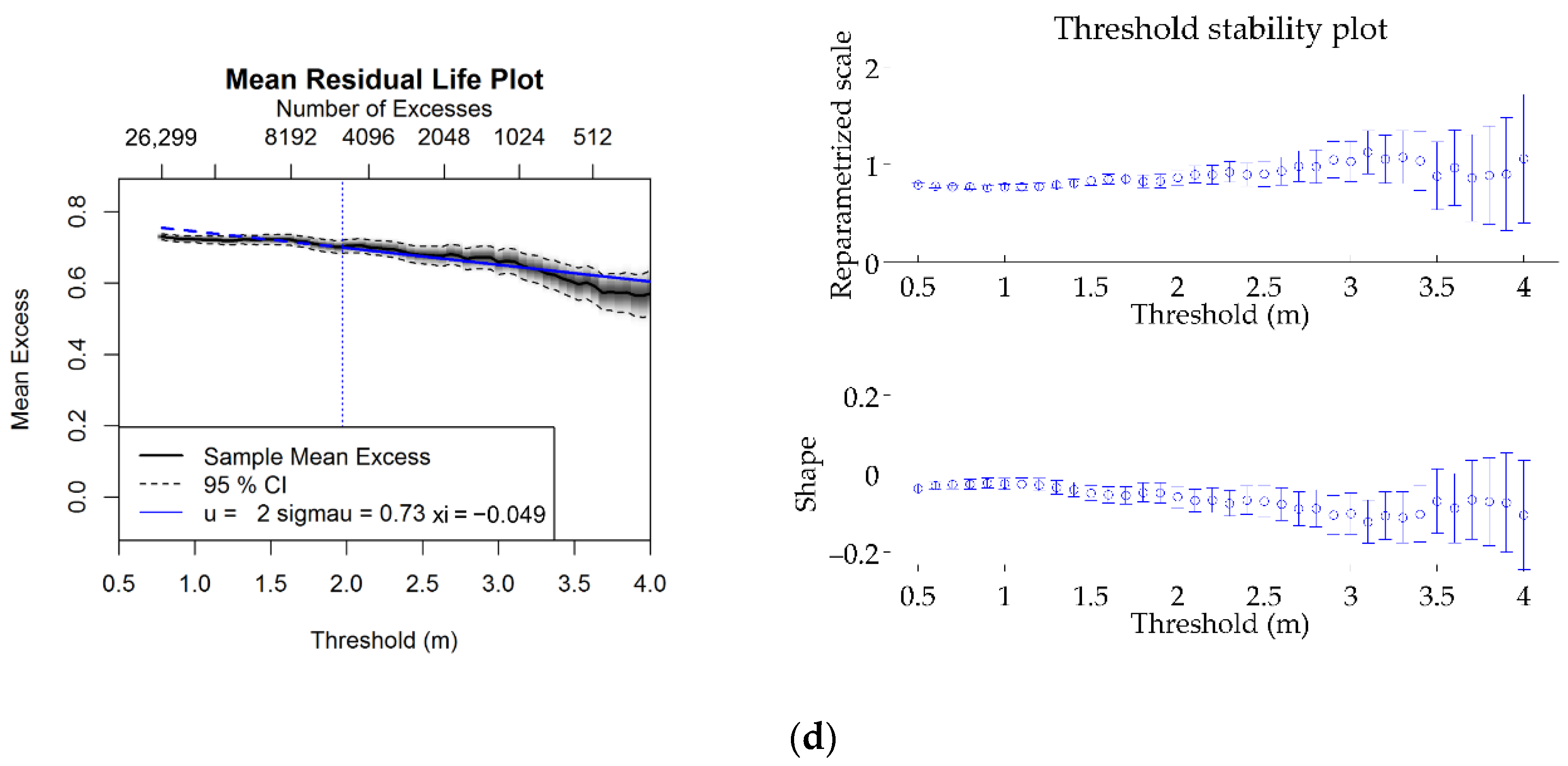
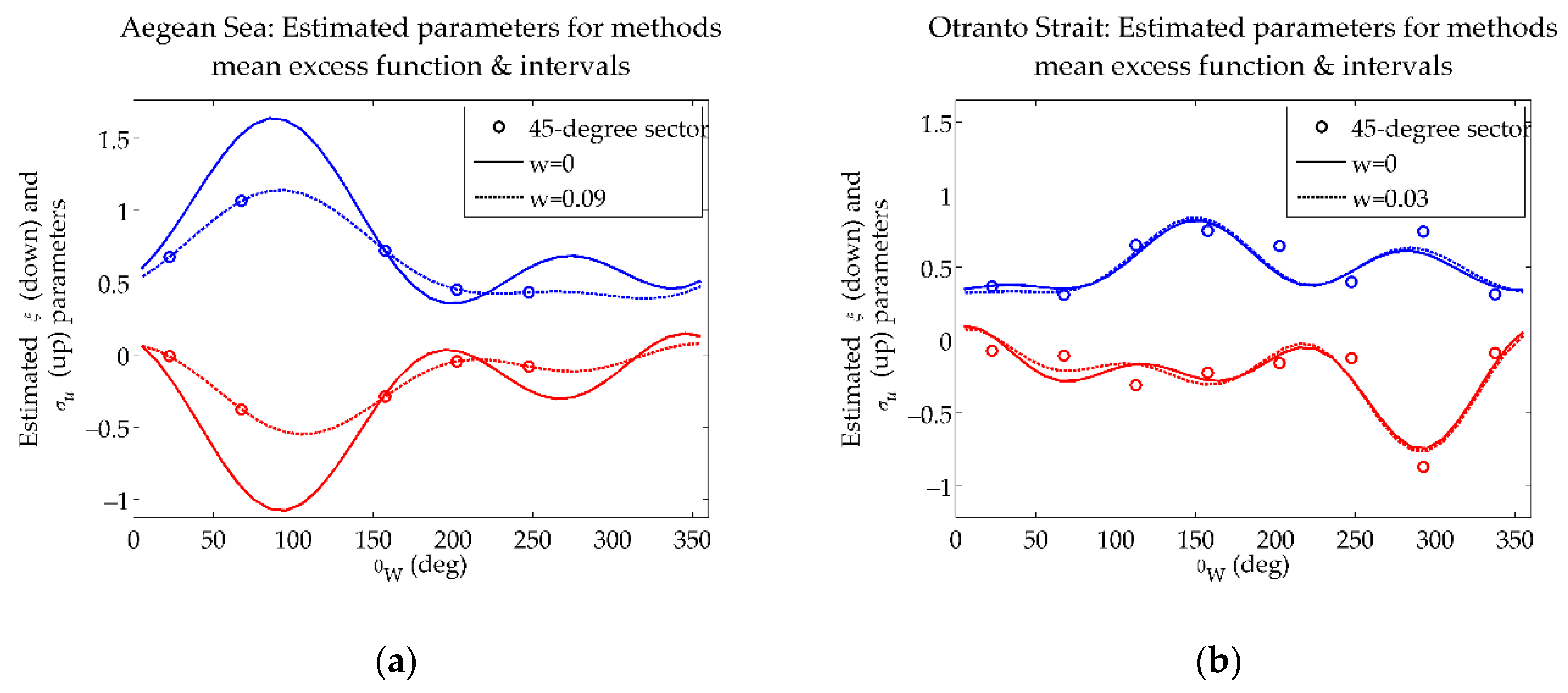
2.3.1. Mean Excess Plot

Following the threshold stability property of the GP distribution (i.e., shape and modified scale parameters remain constant for higher value of the threshold) and supposing that the excesses over a threshold u * follow this distribution, Davison and Smith [45] suggested using the mean of the GP distribution
E [ X u * | X > u * ] = σ u * 1 ξ ,
for ξ < 1 , which is called mean excess (or mean residual life) function of X . For any threshold u > u * , the above expectation takes the form
E [ X u | X > u ] = σ u 1 ξ = σ u * + ξ u 1 ξ ,
which is linear in u with slope ξ / ( 1 ξ ) .
Given an independent and identically distributed (iid) sample X 1 , , X n , an estimator of Equation (12), say e ^ ( u ) , is the empirical mean excess function defined as:
e ^ ( u ) = i = 1 n u ( X i u ) I { X i > u } i = 1 n u I { X i > u } ,
where I { X i > u } = 1 if X > u and 0 otherwise, meaning that it is estimated as the ratio of the sum of the exceedances over the threshold and the total number of observations exceeding the threshold. The properties of mean excess function are described in Hall and Weller [46]. A proper threshold can be obtained by plotting e ^ ( u ) as a function of the threshold u and identifying the lowest value of threshold above which e ^ ( u ) increases approximately linearly. This plot has been implemented in practice by Hogg and Klugman [47], Begueria [48], Sanchez-Arcilla et al. [49], among others.

2.3.2. Threshold Stability Plot

An alternative graphic technique focuses on the stability of parameter estimates for a range of threshold values u ; see Section 4.3.4 of Coles [6]. If a GP model is acceptable for fitting the excesses over a threshold u * , then for increased thresholds, for example, u > u * , the excesses should also follow a GP distribution with the same shape parameter at threshold u * and a new scale parameter. The scale parameter σ u is estimated by σ u = σ u * + ξ ( u u * ) . The modified scale parameter can be reparametrized as σ u ξ u , which is constant with respect to u . Consequently, the estimates of the shape and modified scale parameters remain constant above u * , if excesses follow the GP distribution with u * being a valid threshold.
Estimates of the shape and the modified scale parameters are plotted against u and the appropriate threshold corresponds to the lowest threshold value for which these estimates are nearly constant. Mean excess and threshold stability plots can be applied simultaneously to obtain the optimum threshold. The main drawbacks of the above graphic approaches as a method of threshold selection is that they require expertise from the analyst for the interpretation of these diagnostics and they can be quite subjective. In addition, as a non-automated method, it is not suggested when multiple locations need to be examined in the context of extreme value analysis.

2.3.3. Percentiles

Among the most common rules of thumb used to derive threshold values is the percentiles (or quantile method). After specifying the appropriate percentile value, the threshold is selected so that it corresponds to the percentile of the time series in hand. For example, the 95% percentile represents the value of the significant wave height that exceeds the 95% of the corresponding ordered sample and this value is selected as threshold. Despite its simplicity, the main drawback is the subjectivity involved. In the relevant literature, a range of percentiles has been proposed. For instance, Dumouchel [50] suggested the upper threshold of 10% but with inadequate theoretical justification, while Eastoe and Tawn [51] used the 95% percentile for river flow data. Grabemann and Weisse [52] chose to represent extreme conditions of wind speed and significant wave height by applying the 99th percentile, while in Arns et al. [53], percentiles varying between the 97.5th and the 99.7th percentile were examined in order to derive the most appropriate threshold for water level data from tide gauge records in various locations; the 99.7th percentile was identified as the most appropriate for the examined study areas.

2.4. Methods for Declustering

Regarding the extreme values of metocean parameters, it is valid that if the time step of the series is smaller than a typical duration of an extreme event (i.e., storm) then they occur in clusters, implying that there is temporal correlation between sequential values. However, in order to apply the POT method, it is essential to ensure that there is mutual independence between extreme events. The prerequisite of independence is achieved by means of declustering, a method that takes out the dependent observations from a correlated series of extreme events so that independent threshold exceedances are extracted reasonably. An alternative term for this method, usually adopted in hydrological studies, is ‘meteorological independence criterion’ [54,55]. This approach was implicitly applied first by Davenport [56] and its main principle is to select the maximum value between consecutive up- and down-crossings of the mean. Several declustering techniques have been developed in the context of extreme value analysis and the outline of this procedure is summarized below:
  • Define clusters of observations in case of consecutive exceedances based on an empirical criterion or parametric models (e.g., Markov chain models, Bartlett-Lewis process).
  • Identify the highest value in each cluster, called declustered peaks.
  • Assume the declustered peaks are independent and fit GP distribution to these peaks.
It is evident that the definition of the cluster entails some degree of subjectivity or arbitrariness, especially when empirical rules are applied, affecting in turn the results. On the other hand, in Davison and Smith [45] it was stated that if a reasonable selection is made as regards the average number of clusters per unit time for the identification of clusters then the results seem to be insensitive to this precise value. A brief overview of the most commonly used declustering methods for POT models is provided below.

2.4.1. Runs Declustering Method

Runs declustering method, described by Smith and Weissman [57], assumes that successive threshold exceedances form a separate cluster as long as their duration does not surpass a set run length, that is, a predefined minimum interval between two successive peaks indicating the termination of a cluster. As in the case of the threshold selection u , there is no formal procedure for the selection of run length; thus, in order to avoid improper choices of run length, which may lead to bias or high variance, the choice of the run length relies on the commonsense experience and the physical background that governs the variable of interest. For instance, when studying ocean waves variables, the run length should be large enough so that the entire duration of fully developed sea states is included. In the relevant literature, a run length of 30h to 96h is chosen to ensure independence between the declustered peaks [58,59,60,61,62,63].

2.4.2. Intervals Declustering Method

A more sophisticated and automatic declustering scheme was developed by Ferro and Segers [64] with the aim of determining the run length directly from the data. It is based on the a priori estimation of the extremal index θ u , θ u [ 0 , 1 ] , which measures the degree of the extreme events to cluster in a stationary process, with θ u = 1 denoting independent extreme data. The extremal index has a direct physical meaning since the inverse of θ u roughly corresponds to the mean cluster size. A review of estimation methods for the extremal index can be found in Ferreira [65] and Moloney et al. [66].
The main difference with runs declustering method is that it does not involve any arbitrary choice in the process of obtaining independent clusters of exceedances and that the automation of the technique lies in the interconnection of threshold selection and declustering, meaning that a different extremal index is chosen with changes in the POT threshold. This approach has been applied by Acero et al. [67] Cebrian and Abaurrea [68] and Della-Marta et al. [69], among others.

2.4.3. Declustering Algorithm (DeCA)

In the context of acquiring statistically independent values of significant wave height, a declustering method was developed by Soukissian and Kalantzi [43] that detects sequences of almost independent maxima from the initial time series in hand based on the physical features of a sea-state system. Specifically, large wave energy reductions between local maximum and subsequent minimum values of significant wave height imply the transition to a different sea-state system and hence leads to the identification of clusters of extreme events from the data series that are ”physically” independent. After a filtering procedure of the initial time series using monotonicity for the detection and removal of stationary sequences, the local maxima and minima are identified and then the corresponding wave energy differences are calculated. If the wave energy reduction is lower than a predefined percentage, then it is considered that the examined sea-state system has ended, forming thus a separate independent cluster. Again, the maximum value within each cluster is extracted to fit the GP model. A rational selection of energy reduction percentage is over 80% that was also adopted in that work. The use of this declustering technique can be also found in Soukissian and Arapi [70].

3. Uncertainty Quantification

The estimation of the uncertainties of the extreme values parameters and the design values were based on the bootstrapping technique, introduced by Efron [71], and it was used due to its generality and its automatic implementation. Various bootstrap methods have been reviewed by Tajvidi [72] for the construction of confidence intervals for the GP distribution parameters and quantiles and it was concluded that for small sample sizes none of the bootstrap methods gives satisfactory results. Moreover, Coles and Simiu [73] proposed an empirical correction of the bootstrap estimates, based on a bias correction to the bootstrap parameter estimates, since there is a tendency of the bootstrap procedure to provide generally shorter tails than the one from the original time series. In this respect, the bias-corrected and accelerated (BCA) bootstrap method, developed by Efron [74], is applied in this work since it attempts to correct for both bias and skewness in the distribution of bootstrap estimates; for more details, see Efron and Tibshirani [75].
Suppose that h is the parameter of interest and let denote by h ^ * a bootstrap replication of h ^ obtained by resampling with replacement from the original data sample. The underlying assumption of BCA method is that a monotone transformation ϕ = m ( h ) exists such that ϕ ^ ~ N ( ϕ z 0 ( 1 + a ϕ ) , ( 1 + a ϕ ) 2 ) , where z 0 and a are the bias-correction and acceleration constants, respectively. The former constant is related to the proportion of bootstrap estimates that are less than the corresponding estimate of the original sample and its estimate can be provided by
z ^ 0 = Φ 1 { # h ^ * ( r ) < h ^ R } ,
with Φ denoting the standard normal cumulative distribution function and r = 1 , 2 , , R denoting each bootstrap sample with total number of bootstrap samples R . The latter correction is proportional to the skewness of the bootstrap distribution and can obtained by the jackknife method. Let h ^ ( i ) , i = 1 , , n , denote the value of the estimate based on the entire original data sample apart from the i th observation. An estimate of the acceleration constant is given by
a ^ = i = 1 n ( h ^ ( · ) h ^ ( i ) ) 3 6 [ i = 1 n ( h ^ ( · ) h ^ ( i ) ) 2 ] 1.5 ,
where h ^ ( · ) = n 1 i = 1 n h ^ ( i ) .
Having the values of z ^ 0 and a ^ , the interval of BCA method is given by ( h ^ ( α 1 ) , h ^ ( α 2 ) ) , where α 1 = Φ ( z ^ 0 + z ^ 0 + z ( α ) 1 a ^ ( z ^ 0 + z ( α ) ) ) and α 2 = Φ ( z ^ 0 + z ^ 0 + z ( 1 α ) 1 a ^ ( z ^ 0 + z ( 1 α ) ) ) with z ( α ) the 100 α th percentile point of a standard normal distribution.
Given the original (random) sample of pairs of one linear and one directional variable ( x , θ ) , say { s i } i = 1 n , the procedure of the adopted bootstrapping is summarized in the following steps for estimating the confidence intervals of the extreme value parameters:
  • Step 1: Estimate the unknown parameters ( σ ^ u , ξ ^ ) of the GP distribution (as functions of θ ) from the initial sample using the ML method described above.
  • Step 2: Create r (random) samples { s i ( r ) } i = 1 n , r = 1 , , R , by random resampling with replacement from the initial sample and obtain the estimates ( σ ^ u * , ξ ^ * ) .
  • Step 3: Repeat step 2 for a large number R . The minimum number of bootstrap sample R for the calculation of reliable confidence intervals is 1000, as is suggested by various studies that address modelling of extremes of environmental parameters; see, for example, Kysely [76], Panagoulia, et al. [77] and Soukissian and Tsalis [78].
  • Step 4: Estimate the two constants of BCA bootstrap method, z ^ 0 and a ^ for each unknown parameter. Then estimate the lower and upper limits σ ^ u ( α 1 ) , ξ ^ ( α 1 ) and σ ^ u ( α 2 ) , ξ ^ ( α 2 ) , respectively.

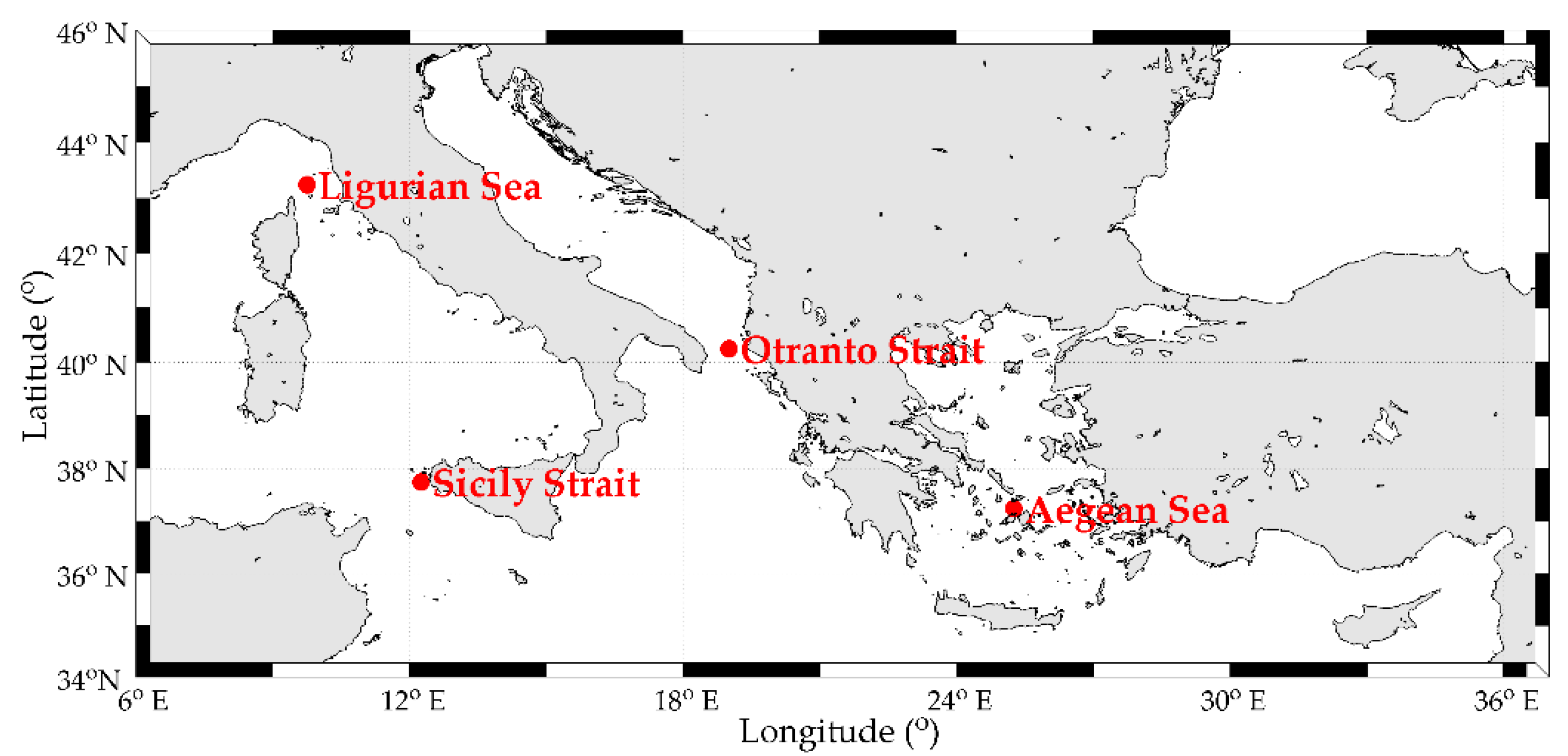
4. Description of Wave Data

Reanalysis wave data from the ERA-Interim database for four grid points located in the Eastern Mediterranean Sea were used. The wave parameters that were obtained for the purposes of this work were the significant wave height H S and the mean wave direction θ W . The geographical coordinates, the measurement period and the sample size of each grid point are listed in Table 1; see also Figure 2. The three areas (Aegean Sea, Otranto Strait and Sicily Strait) were selected as indicative locations with high wave energy flux and relatively low variability in the Mediterranean Sea; see, for example, Besio et al. [79]. On the contrary, Ligurian Sea is one of the most active areas of cyclogenesis in the Mediterranean. Moreover, this area is characterized by very strong and rapid variability of meteorological conditions [80].
The statistical parameters that are examined for H S are the mean value m H S , median m e d H S , minimum min H S and maximum max H S values, standard deviation s H S , coefficient of variation C V H S , skewness S k H S and kurtosis K u H S . The results for all these parameters are presented in Table 2. The locations Aegean Sea and Sicily Strait are characterized by the highest mean and median values of H S (1 m and 0.8 m, respectively), while in the latter location the maximum value of H S is encountered (6.4 m). On the other hand, the location Otranto Strait presents the highest values of S k H S and K u H S , denoting a highly right skewed distribution of H S and rather heavy tails.
In Table 3, the values of some basic circular (statistical) parameters (i.e., mean direction m θ W , mean resultant length R ¯ θ W , circular variance V θ W , circular standard deviation s θ W , skewness S k θ W , kurtosis K u θ W ) as regards wave direction are presented. The definitions of the above parameters can be found in Fisher [81]. It is noticed that the mean wave direction at Ligurian Sea and Sicily Strait (both located western of Italy) is coming from the western sector, while at Aegean Sea and Otranto Strait the mean direction of wave propagation is from the northern and south-eastern, respectively. Moreover, Aegean Sea has the highest value of R ¯ θ W (0.42) and the lowest value of V θ W (0.58), respectively, denoting quite concentrated data at a particular directional sector. The lowest absolute values for S k θ W (0.18) and K u θ W (0.20) are encountered at Ligurian Sea and Sicily Strait, respectively, implying that the corresponding dataset is rather multimodal.
In Figure 3, the bivariate histograms of H S and θ W are provided for each location. From these histograms it is clear that there is a strong dependence between the two wave characteristics, especially for particular directional sectors. For instance, for all locations, except for Ligurian Sea, the northern sector is highly associated with low (for Otranto Strait) to medium values of H S (for Aegean Sea and Sicily Strait), while Otranto Strait and Sicily Strait present moderate dependence of H S with other directional sectors as well.

5. Numerical Results

5.1. Preliminary Results

For each examined location, seven different combinations of the methods for threshold selection and declustering are performed. Each of the threshold selection methods (i.e., mean excess function, threshold stability plot, percentile) is combined with runs and intervals declustering methods along with DeCA declustering method. For the latter method, the threshold is obtained as the median of the declustered values. Firstly, the threshold values of H S are estimated irrespective of θ W . After a sensitivity analysis, the 95th percentile was used to derive threshold values, since higher percentiles provided a smaller sample of extreme data that result in large variance [82]. As regards threshold values from mean excess and threshold stability plots, the packages ‘evmix v2.11′ and ‘extRemes v2.0.10′ in R were used, respectively; the corresponding graphs are provided in Figure 4. In Table 4, the threshold values of H S for each location and method are summarized. The maximum threshold values are systematically provided by the DeCA method, while the minimum ones from the mean excess. It is obvious from the mean excess plots of all locations that the decreasing behavior of the mean excess function shows that the higher we go in the sample data, the lower the excess values are, indicating a thin-tailed behavior of the distribution.
In Table 5, the number of exceedances for H S after implementing the declustering methods for each threshold selection method is provided for the examined locations. These H S exceedances along with the corresponding values of θ W are used for fitting the directional extreme value model described in Section 2. Let it be noted that for runs declustering, a run length of 36h was chosen as the most representative for the examined locations, providing sufficient data for the subsequent analysis. Mean excess function and intervals declustering method provide systematically the largest number of exceedances for all locations. On the other hand, DeCA provides the smallest one, rendering its position disadvantageous in the directional extreme value analysis, since a sufficient number of exceedances (>20 ( H S ,   θ W ) pairs of extreme values) is preferred for each 45-degree sector in order to obtain reliable results from the GP distribution fit.
With the final exceedances in hand, the LR test was performed to determine the order of the Fourier model that sufficiently describes the variability of the extreme value parameters for each location. As shown in Table 6, the majority of the considered combinations of methods for threshold selection and declustering for the examined locations concerns the first order Fourier model apart from Otranto Strait, where the higher order model indicates its directional complexity (see also Section 4). Let it be noted that the initial values for the ML approach are obtained by estimating the parameters of the Fourier model from the independent fits by least squares method, which implies a sufficient number of equations according to the number of the unknown parameters (i.e., the order of the Fourier model). Thus, in order to ensure a fair comparison between the combinations of the abovementioned methods, when the number of the 45-degree width sectors with sufficient number of exceedances (>20) was less than three (out of eight) for the first order Fourier model, the corresponding combination of methods was omitted from the analysis. The restriction for the second and third order models is five and seven sectors, respectively. The results of Table 6 in italics denote the combinations of methods that satisfy these two restrictions. DeCA method is not included henceforth because even for the first order model, the sectors satisfying the above conditions was less than three.
In the estimation of parameters with the penalized ML, an additional constant w needs to be determined. This constant is estimated based on the minimum value of mean absolute error between the estimated parameters from the directional extreme model and the ones obtained by the independent fits from the successive directional sectors of 45-degree width, provided simultaneously for both extreme parameters ξ and σ u . The obtained results are shown within the parenthesis in Table 6.
In Figure 5, the proposed directional extreme value model (dashed line) is provided along with the standard directional model (solid line), which does not consider the penalty term for the estimation of parameters (i.e., w = 0 ), for Aegean Sea and Otranto Strait locations. From Figure 5, it is shown that the estimates obtained from the proposed model provide better results than the standard directional model, when compared with the estimates derived from the independent fits of successive sectors with width 45° (indicated by circles), even for a small weighting constant. Note these two examples consider different order for the Fourier model and different weighting constants w . From these preliminary results at the selected locations, it is evident that both the use of the directional extreme value model and the inclusion of the penalty term in ML method are important for the reliable estimation of the design values of H S and the confidence intervals.
In Figure 6, the cdfs obtained from the directional extreme value model with and without the inclusion of the penalty term along with the empirical cdf are presented for Aegean Sea and Otranto Strait locations. For the latter location, both cdfs have a similar behavior while for the former one, the cdf with the penalty term overestimates the empirical one.

5.2. Final Results

In this section, we focus on the estimation of the design values of H S for 50- and 100-year return period for the combination of methods that provide the largest sample size of exceedances, that is, the mean excess function for threshold selection and the intervals declustering method. In Table 7, Table 8, Table 9 and Table 10, the values of the estimates and the corresponding 97.5% confidence intervals using the BCA bootstrap method, with 2000 bootstrap resamples, are given for all locations. As was concluded by Coles and Simiu [73], bootstrapping can provide reliable and realistic estimates for uncertainties in extreme value analysis if carefully implemented.
Figure 7 shows H S design values with direction for the 50-year return period by considering three different approaches; the blue solid line represents the estimates from the proposed directional model, the green dashed line represents the estimate obtained by the GP distribution without the consideration of the directional complexity of its parameters (omni-directional case) and the red circles represent the estimates from the independent fits of the eight consecutive directional sectors. These results along with the 97.5% confidence intervals are also depicted in Figure 8b, Figure 9b, Figure 10b and Figure 11b. Note that in order to assure consistency between the results from the omni-directional case and the indep8endent fits from each directional sector, the return period is multiplied by the number of sectors as was suggested by Forristall [42]. In this way, the product of the probabilities obtained from each sector equals the probability of non-exceedance from the omni-directional criterion. For all locations, the design value obtained from the standard GP fit is lower compared to the estimates provided at the peaks of the directional model. Moreover, the design values estimated by the sectors with the largest number of observations are always higher than the corresponding design value obtained from the standard GP fit. The performance of the proposed directional model is apparently very satisfactory for Aegean Sea and Otranto Strait (Figure 7a,c, respectively), while for the rest of the locations, this model seems to provide consistently higher design values for H S when compared with the independent fits. A possible explanation could be the low order of the Fourier model; see also Figure 9b and Figure 11b, where the range of the lower bounds of confidence intervals is relatively high.
In Figure 8a, Figure 9a, Figure 10a and Figure 11a, the wave rose diagrams of H S and θ W representing the exceedances (as a frequency of occurrence) obtained from the implementation of mean excess function for threshold selection and the intervals declustering method are presented for all locations. In Figure 8b,c, Figure 9b,c, Figure 10b,c, and Figure 11b,c. the 50- and 100-year H S design values are shown along the 97.5% confidence intervals estimated by the BCA method. These levels seem reasonable when considering that the expected lifetime of WECs is 20–25 years on average [83]. A general remark concerning all locations is that the range between the H S design value and the upper bounds is much smaller than the corresponding range with the lower bounds. Another remarkable result is that in two locations it is not expected to encounter extreme H S values from the dominant directional sector but from the next one, which may have a more limited amount of data. Since the results of the 50- and 100-year return period are similar, the following comments can be summarized for both return periods per location:
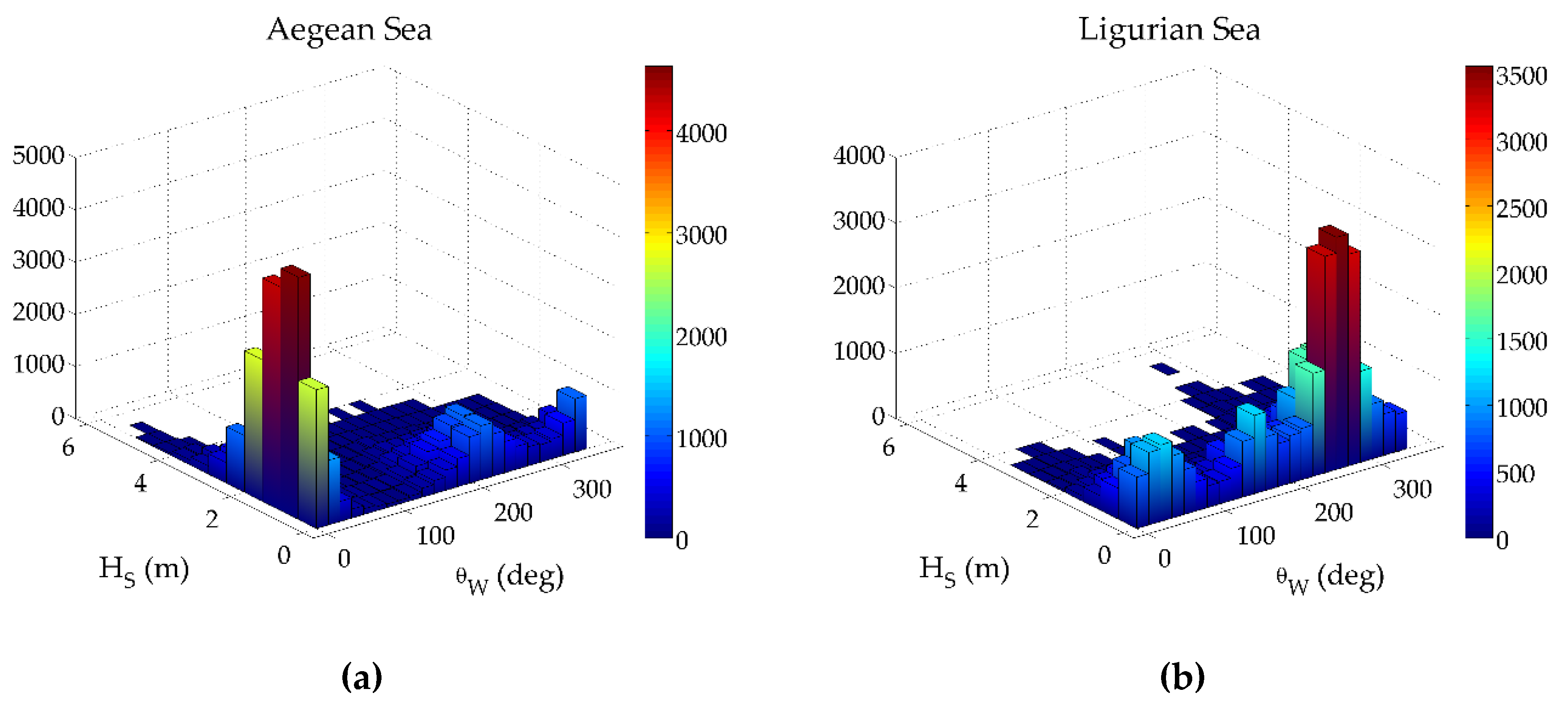
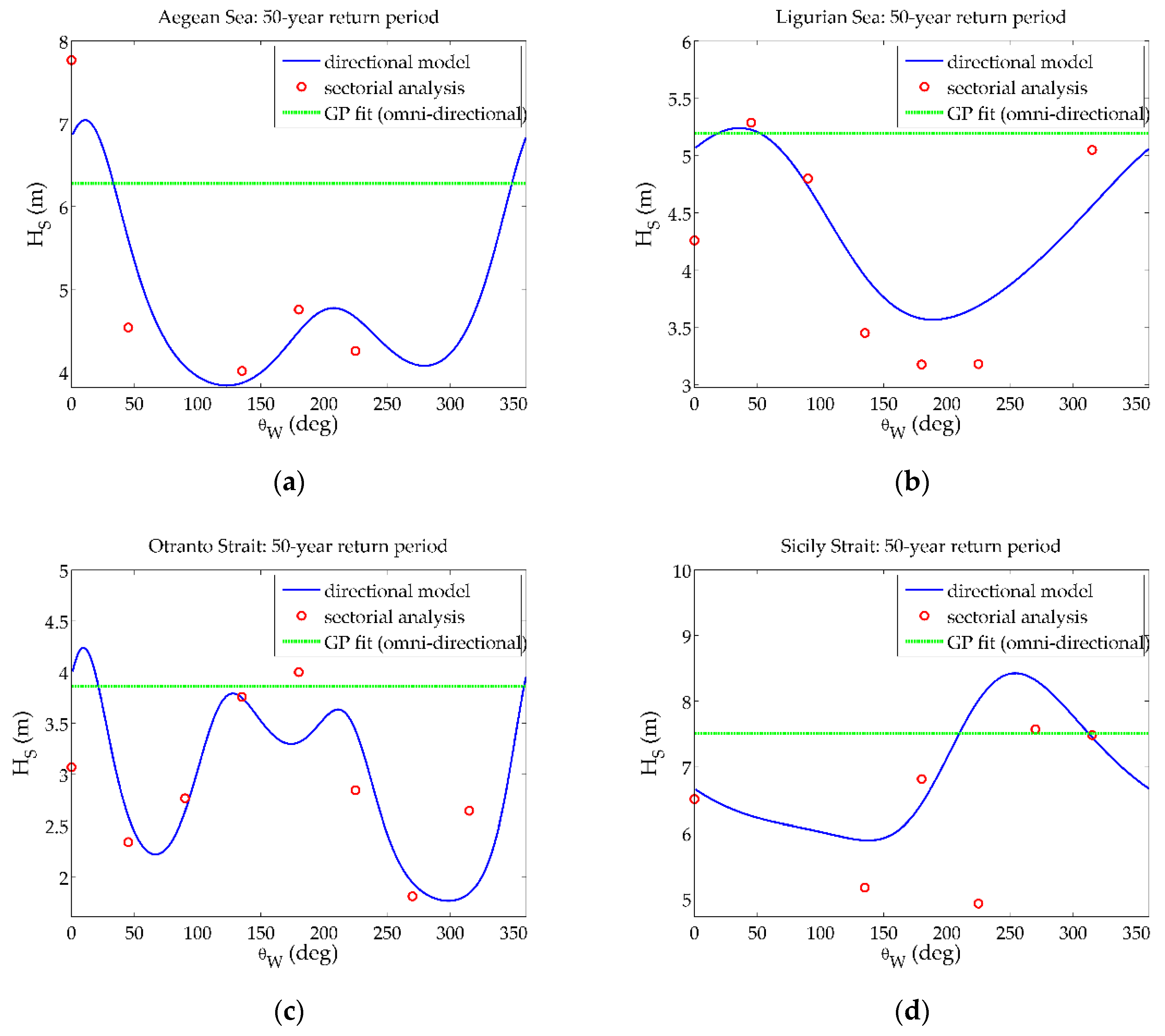
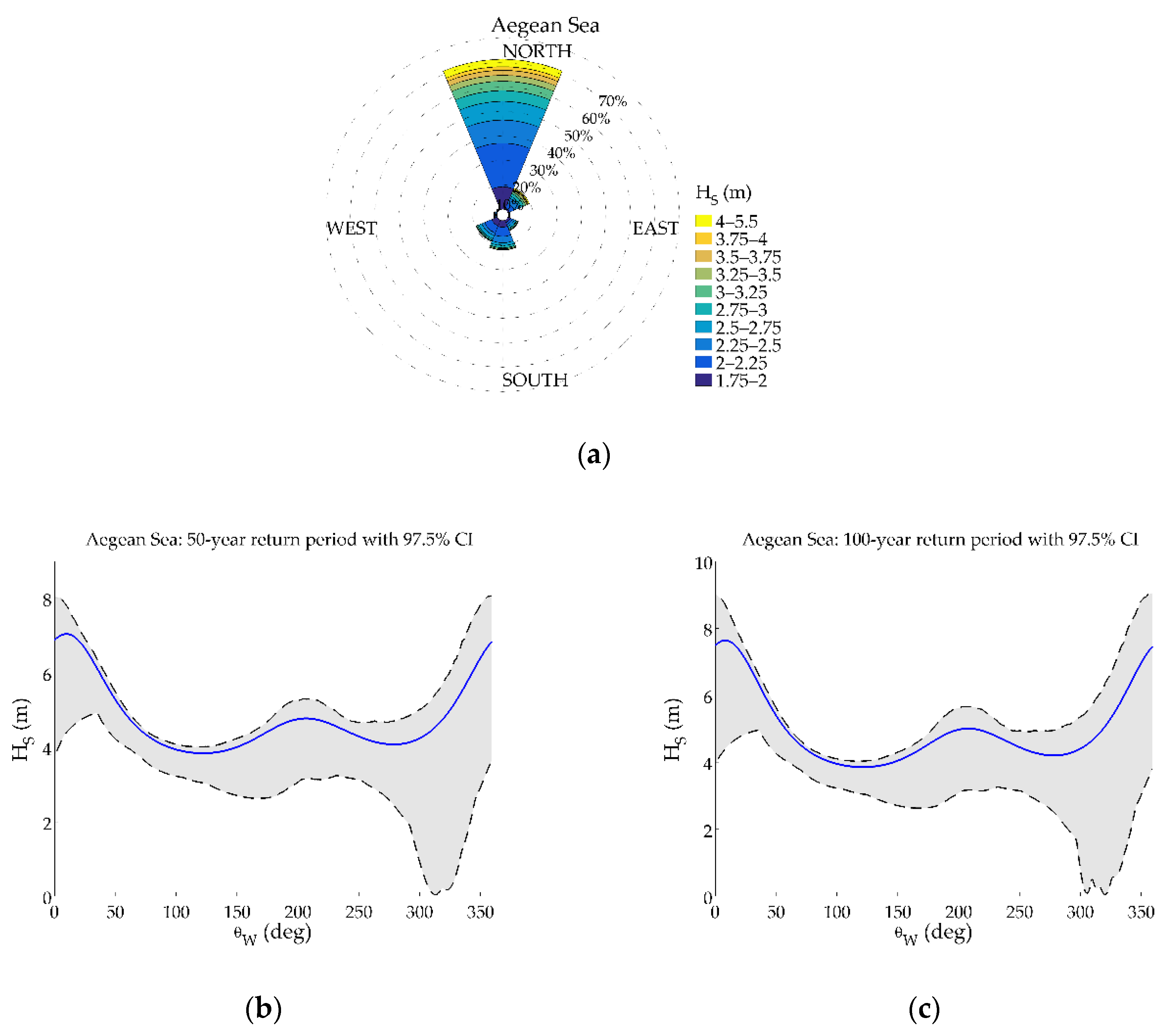
  • For Aegean Sea, the dominant sector for extreme wave heights is the northern one, probably attributed to the Etesian winds, which gives extreme values up to 7 m at this sector and lower values characterize the rest directional sectors (e.g., for the sector [ 50 ° , 310 ° ] the H S value is 4.3 m in the mean) as regards the 50-year return period. Furthermore, the low values of the lower bound of the 97.5% confidence intervals in the north-western sector can be justified by the lack of data obtained from the implementation of the specific combination of methods.
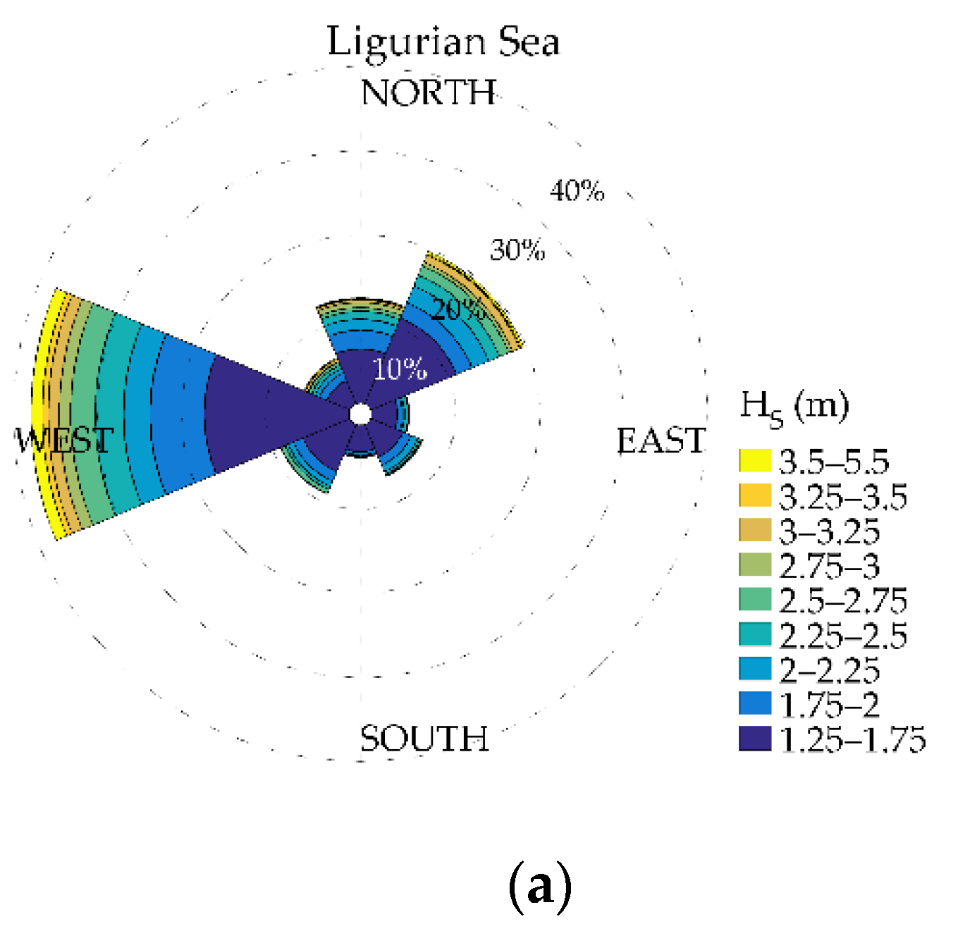
  • For Ligurian Sea, the north-eastern sector is characterized by high values of H S (5.4 m for the 50-year return period), even though it is the second dominant directional sector for H S , while the southern sector, with the least amount of extreme data, provides the lowest values (3.6 m).
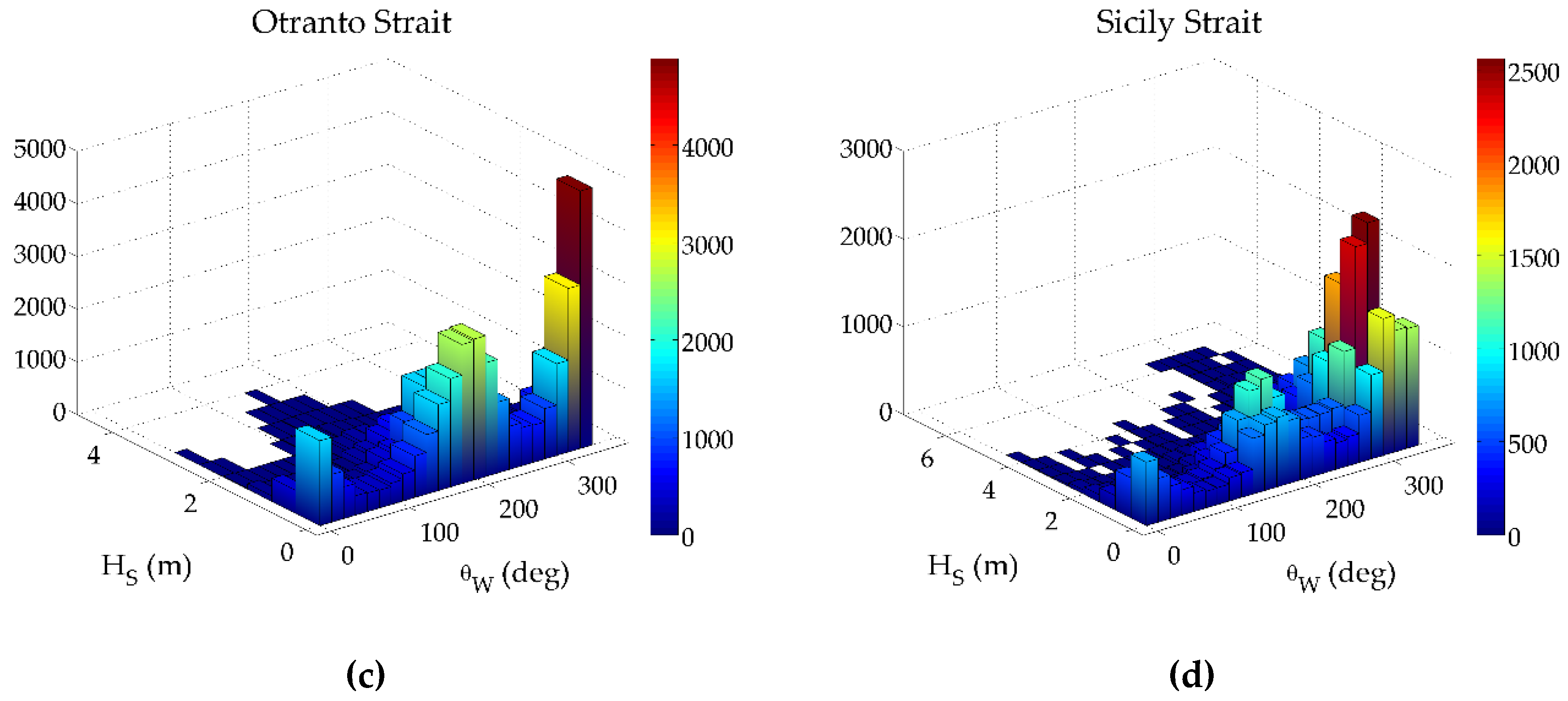
  • For Otranto Strait, the two dominant wave directions (in the south and south-eastern sectors) are translated in two consecutive peaks in the H S design value graphs, while the two concave forms (in the north-eastern and western sectors) correspond to the sectors with the minimum amount of extreme data. Let note that the form of the lower bounds differs from the H S design value.
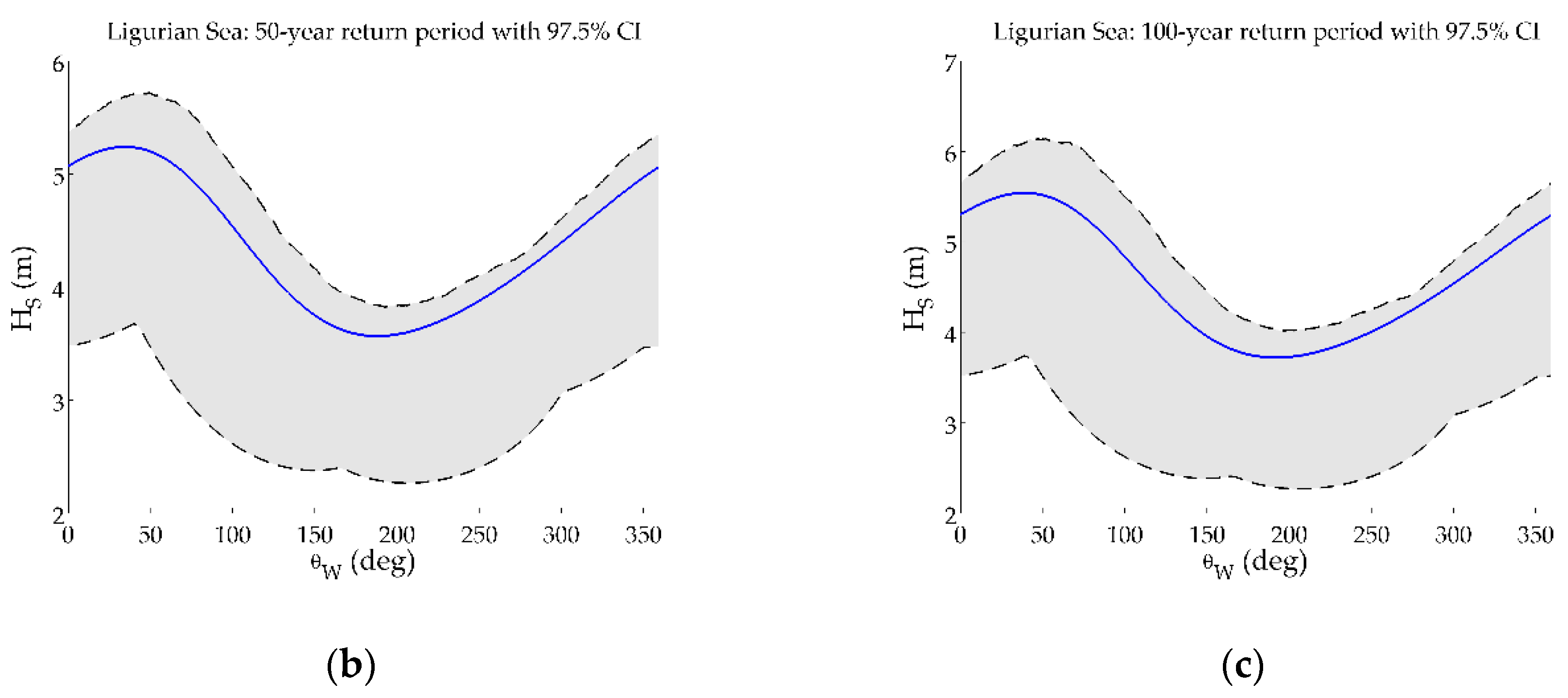
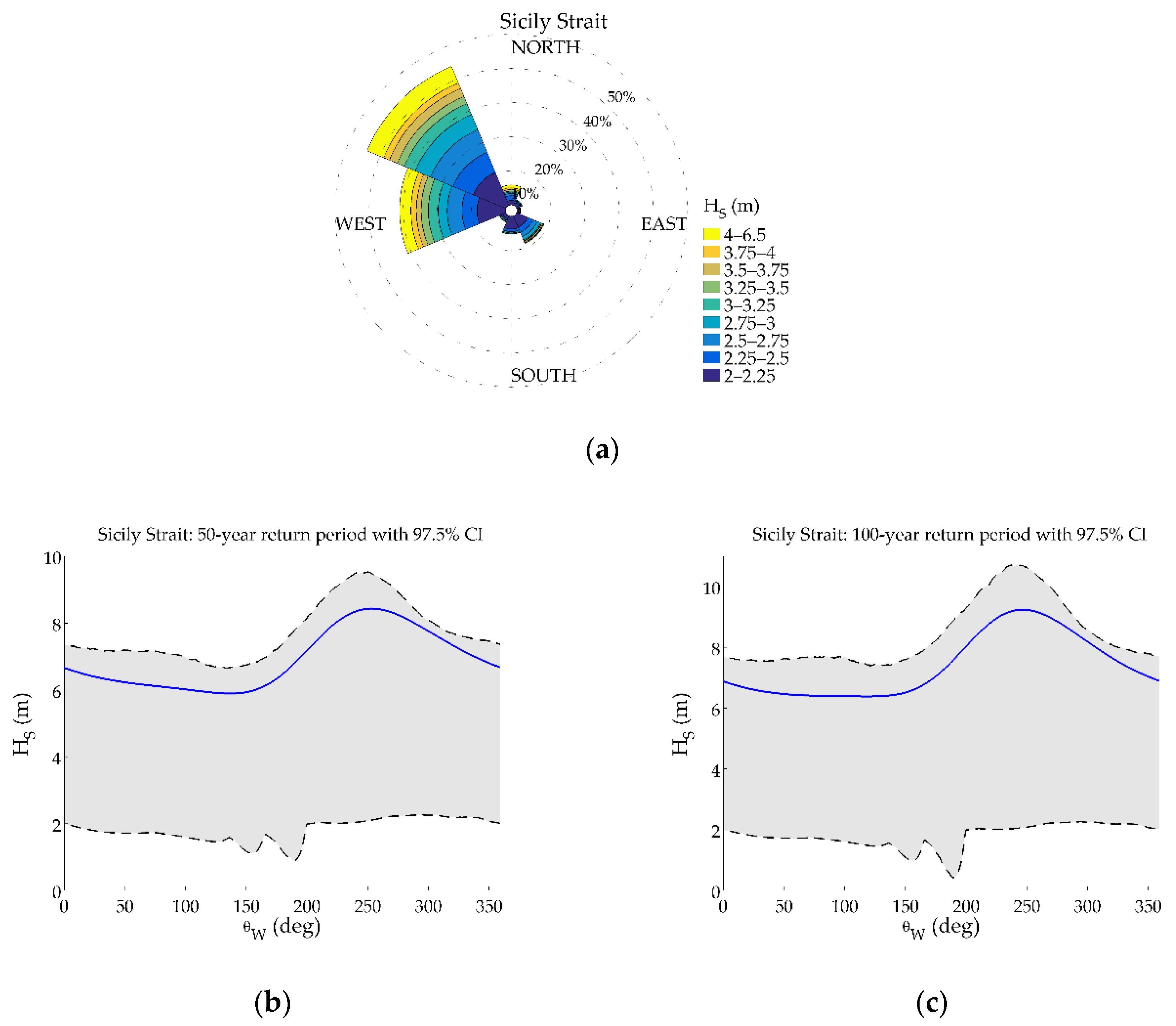
  • For Sicily Strait, the location with the most intense sea states according to the analyzed hindcast wave data, the second dominant directional sector for H S (i.e., the western) is characterized by the highest H S design values (8.4 m for the 50-year return period) and the lowest values are observed for the south-eastern sector (5.9 m for the 50-year return period). The largest difference between the lower bounds of the confidence interval and the H S design value is close to 6.3 m for the 50-year return period encountered in the south-western sector.

6. Conclusions

Estimation of design values of wave parameters by means of directional extreme value models can be in favor of extreme value models that ignore direction in wave energy applications, where the consideration of directionality is crucial in the design of marine structures. With the increasing availability of long-term directional metocean data mainly from numerical models, it is strongly advised to take advantage of directional extreme value models in optimizing the performance and costs of marine facilities.
In this analysis, long-term wave data from four locations in the eastern Mediterranean Sea were analyzed. Three threshold selection and two declustering methods were combined to examine the corresponding effect in the determination of the order of the Fourier model and in turn, in the parameter estimates and design values and their uncertainties. After selecting the appropriate threshold for each method for the identification of extreme wave heights and applying the proposed declustering techniques due to the prerequisite of independence, a Fourier form was used to model the parameters of the Generalized Pareto distribution as a smooth function of wave direction. A penalized maximum likelihood was implemented to estimate extreme parameters and ensure consistency with the directionally independent fits. In the majority of the combinations of methods, the first order Fourier series model was found to be adequate for the description of extreme wave heights with direction, while higher order models were necessary particularly for locations with more complex directional features, like the location in the Ligurian Sea. Directional design values of significant wave height were provided for the 50- and 100-year period as an objective criterion for design specification purposes and predict reliable extreme wave conditions during the lifetime of a wave energy facility. Confidence intervals of 97.5% were also provided by the bias-corrected and accelerated bootstrap method.
The proposed method can be transferred to other locations as well, provided that there are enough data in each directional sector (at least 20) and the non-empty directional sectors are adequate according to the order of the Fourier model. For example, the first order model requires at least three non-empty directional sectors. Therefore, the application of the proposed methodology should be made with caution in order to satisfy all the above mentioned requirements. Finally, the present analysis may be useful in other applications related to marine renewable energy sectors, such as the offshore wind sector and coastal engineering studies (e.g., coastal erosion/accretion studies due to wave action coming from multiple directions). Interesting future research directions include the consideration of alternative models to Fourier series expansion for expressing smoothly the periodicity of the parameters in terms of direction, while a pre-defined threshold that is directionally varying would also be meaningful. Moreover, the effects of selecting various numbers of sectors, either equiangular or not, for the independent fits deserve a thorough investigation.

Author Contributions

F.K. contributed to methodology, analysis, data curation, investigation, literature review, original draft preparation, T.S. and K.B. contributed to conceptualization, methodology, supervision and review and editing of manuscript. All authors have read and agreed to the published version of the manuscript.

Funding

This research was funded by national and EU funds under National Strategic Reference Framework 2014-2020 in the framework of the project titled “Blue Growth with Innovation and application in the Greek Seas —GLAFKI” (MIS 5002438).

Conflicts of Interest

The authors declare no conflict of interest.

References

  1. Naess, A. Statistical extrapolation of extreme value data based on the peaks over threshold method. J. Offshore Mech. Arct. 1998, 120, 91–96. [Google Scholar] [CrossRef]
  2. Caires, S.; Sterl, A. 100-year return value estimates for ocean wind speed and significant wave height from the ERA-40 data. J. Clim. 2005, 18, 1032–1048. [Google Scholar] [CrossRef]
  3. Soukissian, T.H.; Kalantzi, G. Extreme value analysis methods used for wave prediction. In Proceedings of the 16th International Offshore and Polar Engineering Conference, San Francisco, CA, USA, 28 May–2 June 2006; pp. 10–17. [Google Scholar]
  4. Caires, S. A Comparative Simulation Study of the Annual Maxima and the Peaks-over-Threshold Methods; Technical report, SBW-Belastingen: Subproject “Statistics”. Deltares Report 1200264-002; Deltares: Delft, The Netherlands, 2009. [Google Scholar]
  5. Wang, Q.J. The POT Model Described by the Generalized Pareto Distribution with Poisson Arrival Rate. J. Hydrol. 1991, 129, 263–280. [Google Scholar] [CrossRef]
  6. Coles, S. An Introduction to Statistical Modeling of Extreme Values, 1st ed.; Springer: London, UK, 2001. [Google Scholar] [CrossRef]
  7. Leadbetter, M.R.; Lindgren, G.; Rootzen, H. Extremes and Related Properties of Random Sequences and Processes, 1st ed.; Springer: New York, NY, USA, 1983. [Google Scholar]
  8. Balkema, A.A.; de Haan, L. Residual Life Time at Great Age. Ann. Probab. 1974, 2, 792–804. [Google Scholar] [CrossRef]
  9. Pickands, J. Statistical inference using extreme order statistics. Ann. Stat. 1975, 3, 119–131. [Google Scholar]
  10. Vanmontfort, M.A.J.; Witter, J.V. Testing Exponentiality against Generalized Pareto Distribution. J. Hydrol. 1985, 78, 305–315. [Google Scholar] [CrossRef]
  11. Rosbjerg, D.; Madsen, H.; Rasmussen, P.F. Prediction in Partial Duration Series with Generalized Pareto-distributed Exceedances. Water Resour. Res. 1992, 28, 3001–3010. [Google Scholar] [CrossRef]
  12. Vogel, R.M.; Mcmahon, T.A.; Chiew, F.H.S. Floodflow Frequency Model Selection in Australia. J. Hydrol. 1993, 146, 421–449. [Google Scholar] [CrossRef]
  13. Katz, R.W.; Parlange, M.B.; Naveau, P. Statistics of extremes in hydrology. Adv. Water Resour. 2002, 25, 1287–1304. [Google Scholar] [CrossRef] [Green Version]
  14. Prudhomme, C.; Jakob, D.; Svensson, C. Uncertainty and climate change impact on the flood regime of small UK catchments. J. Hydrol. 2003, 277, 1–23. [Google Scholar] [CrossRef]
  15. Grimshaw, S.D. Computing Maximum-Likelihood-Estimates for the Generalized Pareto Distribution. Technometrics 1993, 35, 185–191. [Google Scholar] [CrossRef]
  16. Hosking, J.R.M.; Wallis, J.R. Parameter and Quantile Estimation for the Generalized Pareto Distribution. Technometrics 1987, 29, 339–349. [Google Scholar] [CrossRef]
  17. Greenwood, J.A.; Landwehr, J.M.; Matalas, N.C.; Wallis, J.R. Probability Weighted Moments - Definition and Relation to Parameters of Several Distributions Expressable in Inverse Form. Water Resour. Res. 1979, 15, 1049–1054. [Google Scholar] [CrossRef] [Green Version]
  18. Moharram, S.H.; Gosain, A.K.; Kapoor, P.N. A Comparative-Study for the Estimators of the Generalized Pareto Distribution. J. Hydrol. 1993, 150, 169–185. [Google Scholar] [CrossRef]
  19. Castillo, E.; Hadi, A.S. Fitting the generalized Pareto distribution to data. J. Am. Stat. Assoc. 1997, 92, 1609–1620. [Google Scholar] [CrossRef]
  20. Castellanos, M.E.; Cabras, S. A default Bayesian procedure for the generalized Pareto distribution. J. Stat. Plan. Infer. 2007, 137, 473–483. [Google Scholar] [CrossRef]
  21. Bermudez, P.D.; Kotz, S. Parameter estimation of the generalized Pareto distribution-Part II. J. Stat. Plan. Infer. 2010, 140, 1374–1397. [Google Scholar] [CrossRef]
  22. Scarrott, C.; MacDonald, A. A Review of Extreme Value Threshold Estimation and Uncertainty Quantification. Revstat.-Stat. J. 2012, 10, 33–60. [Google Scholar]
  23. Langousis, A.; Mamalakis, A.; Puliga, M.; Deidda, R. Threshold detection for the generalized Pareto distribution: Review of representative methods and application to the NOAA NCDC daily rainfall database. Water Resour. Res. 2016, 52, 2659–2681. [Google Scholar] [CrossRef] [Green Version]
  24. Drees, H.; de Haan, L.; Resnick, S.I. How to make a Hill plot. Ann. Statist. 2000, 28, 254–274. [Google Scholar] [CrossRef]
  25. Choulakian, V.; Stephens, M.A. Goodness-of-fit tests for the generalized Pareto distribution. Technometrics 2001, 43, 478–484. [Google Scholar] [CrossRef]
  26. Northrop, P.J.; Coleman, C.L. Improved threshold diagnostic plots for extreme value analyses. Extremes 2014, 17, 289–303. [Google Scholar] [CrossRef] [Green Version]
  27. ABS. Guide for Load and Resistance Factor Design (LRFD) Criteria for Offshore Structures; American Bureau of Shipping: Houston, TX, USA, 2016. [Google Scholar]
  28. DNV. Recommended Practice DNV-RP-C205: Environmental Conditions and Environmental Loads; Det Norske Veritas AS: Oslo, Norway, 2014. [Google Scholar]
  29. Soukissian, T.H. Probabilistic modeling of directional and linear characteristics of wind and sea states. Ocean. Eng. 2014, 91, 91–110. [Google Scholar] [CrossRef]
  30. Wei, K.; Arwade, S.R.; Myers, A.T.; Valamanesh, V.; Pang, W.C. Effect of wind and wave directionality on the structural performance of non-operational offshore wind turbines supported by jackets during hurricanes. Wind Energy 2017, 20, 289–303. [Google Scholar] [CrossRef]
  31. Soukissian, T.H.; Karathanasi, F.E. On the selection of bivariate parametric models for wind data. Appl. Energy 2017, 188, 280–304. [Google Scholar] [CrossRef]
  32. Moriarty, W.W.; Templeton, J.I. On the Estimation of Extreme Wind Gusts by Direction Sector. J. Wind Eng. Ind. Aerodyn. 1983, 13, 127–138. [Google Scholar] [CrossRef]
  33. Coles, S.G.; Walshaw, D. Directional Modeling of Extreme Wind Speeds. J. R. Stat. Soc. C-App. 1994, 43, 139–157. [Google Scholar]
  34. Simiu, E.; Hendrickson, E.M.; Nolan, W.A.; Olkin, I.; Spiegelman, C.H. Multivariate Distributions of Directional Wind Speeds. J. Struct. Eng.-Asce 1985, 111, 939–943. [Google Scholar] [CrossRef]
  35. Solari, S.; Losada, M.A. Simulation of non-stationary wind speed and direction time series. J. Wind Eng. Ind. Aerodyn. 2016, 149, 48–58. [Google Scholar] [CrossRef]
  36. Folgueras, P.; Solari, S.; Losada, M.A. The selection of directional sectors for the analysis of extreme wind speed. Nat. Hazard. Earth Sys. 2019, 19, 221–236. [Google Scholar] [CrossRef] [Green Version]
  37. Robinson, M.E.; Tawn, J.A. Statistics for extreme sea currents. J. R. Stat. Soc. C-App. 1997, 46, 183–205. [Google Scholar] [CrossRef]
  38. Ewans, K.C.; Jonathan, P. The effect of directionality on extreme wave design criteria. In Proceedings of the 9th International Workshop on Wave Hindcasting and Forecasting, Victoria, BC, Canada, 24–29 September 2006. [Google Scholar]
  39. Ewans, K.; Jonathan, P. The effect of directionality on Northern North Sea extreme wave design criteria. J. Offshore Mech. Arct. Eng. 2008, 130. [Google Scholar] [CrossRef]
  40. Jonathan, P.; Ewans, K. The effect of directionality on extreme wave design criteria. Ocean. Eng. 2007, 34, 1977–1994. [Google Scholar] [CrossRef]
  41. Jonathan, P.; Ewans, K.; Forristall, G. Statistical estimation of extreme ocean environments: The requirement for modelling directionality and other covariate effects. Ocean. Eng. 2008, 35, 1211–1225. [Google Scholar] [CrossRef]
  42. Forristall, G.Z. On the use of directional wave criteria. J. Waterw. Port. Coast. 2004, 130, 272–275. [Google Scholar] [CrossRef]
  43. Soukissian, T.H.; Kalantzi, G.D. A new method for applying r-Largest maxima model for design sea-state prediction. Int. J. Offshore Polar 2009, 19, 176–182. [Google Scholar]
  44. Reiss, R.-D.; Thomas, M. Statistical Analysis of Extreme Ealues, with Application to Insurance, Finance, Hydrology and Other Fields, 3rd ed.; Birkhäuser Verlag: Basel, Switzerland, 2007. [Google Scholar]
  45. Davison, A.C.; Smith, R.L. Models for Exceedances over High Thresholds. J. R. Stat. Soc. B Met. 1990, 52, 393–442. [Google Scholar] [CrossRef]
  46. Hall, W.; Weller, J. Mean residual life. In Statistics and Related Topics; Csorgo, M., Dawson, D.A., Rao, J.N.K., Saleh, A.K.M.E., Eds.; Norrh-Holland Publishing Company: Amsterdam, The Netherlands, 1981; pp. 169–184. [Google Scholar]
  47. Hogg, R.V.; Klugman, S.A. Loss Distributions; Wiley: New York, NY, USA, 1984. [Google Scholar]
  48. Begueria, S. Uncertainties in partial duration series modelling of extremes related to the choice of the threshold value. J. Hydrol. 2005, 303, 215–230. [Google Scholar] [CrossRef] [Green Version]
  49. Sanchez-Arcilla, A.; Aguar, J.G.; Egozcue, J.J.; Ortego, M.I.; Galiatsatou, P.; Prinos, P. Extremes from scarce data: The role of Bayesian and scaling techniques in reducing uncertainty. J. Hydraul. Res. 2008, 46, 224–234. [Google Scholar] [CrossRef]
  50. Dumouchel, W.H. Estimating the stable index-alpha in order to measure tail thickness - a critique. Ann. Stat. 1983, 11, 1019–1031. [Google Scholar] [CrossRef]
  51. Eastoe, E.F.; Tawn, J.A. Modelling the distribution of the cluster maxima of exceedances of subasymptotic thresholds. Biometrika 2012, 99, 43–55. [Google Scholar] [CrossRef]
  52. Grabemann, I.; Weisse, R. Climate change impact on extreme wave conditions in the North Sea: An ensemble study. Ocean. Dynam. 2008, 58, 199–212. [Google Scholar] [CrossRef] [Green Version]
  53. Arns, A.; Wahl, T.; Haigh, I.D.; Jensen, J.; Pattiaratchi, C. Estimating extreme water level probabilities: A comparison of the direct methods and recommendations for best practise. Coast. Eng. 2013, 81, 51–66. [Google Scholar] [CrossRef]
  54. Restrepo-Posada, P.J.; Eagleson, P.S. Identification of Independent Rainstorms. J. Hydrol. 1982, 55, 303–319. [Google Scholar] [CrossRef]
  55. Harley, M. Coastal Storim Definition. In Coastal Storms: Processes and Impacts; Ciavola, P., Coco, G., Eds.; Wiley-Blackwell: Chichester, UK, 2017; p. 288. [Google Scholar]
  56. Davenport, A.G. Note on the distribution of the largest value of a random function with application to gust loading. Proc. Inst. Civ. Eng. 1964, 28, 187–196. [Google Scholar] [CrossRef]
  57. Smith, R.L.; Weissman, I. Estimating the extremal index. J. R. Stat. Soc. B Met. 1994, 56, 515–528. [Google Scholar] [CrossRef] [Green Version]
  58. Morton, I.D.; Bowers, J.; Mould, G. Estimating return period wave heights and wind speeds using a seasonal point process model. Coast. Eng. 1997, 31, 305–326. [Google Scholar] [CrossRef]
  59. Fawcett, L.; Walshaw, D. Improved estimation for temporally clustered extremes. Environmetrics 2007, 18, 173–188. [Google Scholar] [CrossRef]
  60. Kapelonis, Z.G.; Gavriliadis, P.N.; Athanassoulis, G.A. Extreme value analysis of dynamical wave climate projections in the Mediterranean Sea. Procedia Comput. Sci. 2015, 66, 210–219. [Google Scholar] [CrossRef] [Green Version]
  61. Lerma, A.N.; Bulteau, T.; Lecacheux, S.; Idier, D. Spatial variability of extreme wave height along the Atlantic and channel French coast. Ocean. Eng. 2015, 97, 175–185. [Google Scholar] [CrossRef]
  62. Samayam, S.; Laface, V.; Annamalaisamy, S.S.; Arena, F.; Vallam, S.; Gavrilovich, P.V. Assessment of reliability of extreme wave height prediction models. Nat. Hazard. Earth Sys. 2017, 17, 409–421. [Google Scholar] [CrossRef] [Green Version]
  63. Santos, V.M.; Haigh, I.D.; Wahl, T. Spatial and temporal clustering analysis of extreme wave events around the UK coastline. J. Mar. Sci. Eng. 2017, 5. [Google Scholar] [CrossRef]
  64. Ferro, C.A.T.; Segers, J. Inference for clusters of extreme values. J. R. Stat. Soc. B 2003, 65, 545–556. [Google Scholar] [CrossRef]
  65. Ferreira, M. Heuristic tools for the estimation of the extremal index: A comparison of methods. Revstat.-Stat. J. 2018, 16, 115–136. [Google Scholar]
  66. Moloney, N.R.; Faranda, D.; Sato, Y. An overview of the extremal index. Chaos 2019, 29, 022101. [Google Scholar] [CrossRef] [Green Version]
  67. Acero, F.J.; Garcia, J.A.; Gallego, M.C. Peaks-over-threshold study of trends in extreme rainfall over the Iberian Peninsula. J. Clim. 2011, 24, 1089–1105. [Google Scholar] [CrossRef]
  68. Cebrian, A.C.; Abaurrea, J. Drought analysis based on a marked cluster Poisson model. J. Hydrometeorol. 2006, 7, 713–723. [Google Scholar] [CrossRef]
  69. Della-Marta, P.M.; Mathis, H.; Frei, C.; Liniger, M.A.; Kleinn, J.; Appenzeller, C. The return period of wind storms over Europe. Int. J. Climatol. 2009, 29, 437–459. [Google Scholar] [CrossRef]
  70. Soukissian, T.H.; Arapi, P.M. The effect of declustering in the r-largest maxima model for the estimation of Hs -design values. Open Ocean. Eng. J. 2011, 4, 34–43. [Google Scholar] [CrossRef] [Green Version]
  71. Efron, B. Bootstrap methods - another look at the jackknife. Ann. Stat. 1979, 7, 1–26. [Google Scholar] [CrossRef]
  72. Tajvidi, N. Confidence intervals and accuracy estimation for heavy-tailed Generalized Pareto distributions. Extremes 2003, 6, 111–123. [Google Scholar] [CrossRef]
  73. Coles, S.; Simiu, E. Estimating uncertainty in the extreme value analysis of data generated by a hurricane simulation model. J. Eng. Mech.-Asce 2003, 129, 1288–1294. [Google Scholar] [CrossRef]
  74. Efron, B. Better bootstrap confidence intervals. J. Am. Stat. Assoc. 1987, 82, 171–185. [Google Scholar] [CrossRef]
  75. Efron, B.; Tibshirani, R.J. An Introduction to the Bootstrap; Chapman and Hall/CRC: Boca Raton, FL, USA, 1993; p. 456. [Google Scholar]
  76. Kysely, J. A Cautionary Note on the Use of Nonparametric Bootstrap for Estimating Uncertainties in Extreme-Value Models. J. Appl. Meteorol. Clim. 2008, 47, 3236–3251. [Google Scholar] [CrossRef]
  77. Panagoulia, D.; Economou, P.; Caroni, C. Stationary and nonstationary generalized extreme value modelling of extreme precipitation over a mountainous area under climate change. Environmetrics 2014, 25, 29–43. [Google Scholar] [CrossRef]
  78. Soukissian, T.H.; Tsalis, C. Effects of parameter estimation method and sample size in metocean design conditions. Ocean. Eng. 2018, 169, 19–37. [Google Scholar] [CrossRef]
  79. Besio, G.; Mentaschi, L.; Mazzino, A. Wave energy resource assessment in the Mediterranean Sea on the basis of a 35-year hindcast. Energy 2016, 94, 50–63. [Google Scholar] [CrossRef]
  80. Ferretti, G.; Barani, S.; Scafidi, D.; Capello, M.; Cutroneo, L.; Vagge, G.; Besio, G. Near real-time monitoring of significant sea wave height through microseism recordings: An application in the Ligurian Sea (Italy). Ocean. Coast. Manag. 2018, 165, 185–194. [Google Scholar] [CrossRef]
  81. Fisher, N.I. Statistical Analysis of Circular Data, 1st ed.; Cambridge University Press: Cambridge, UK, 1993; p. 294. [Google Scholar]
  82. Mudersbach, C.; Wahl, T.; Haigh, I.D.; Jensen, J. Trends in high sea levels of German North Sea gauges compared to regional mean sea level changes. Cont. Shelf Res. 2013, 65, 111–120. [Google Scholar] [CrossRef]
  83. Penalba, M.; Ulazia, A.; Ibarra-Berastegui, G.; Ringwood, J.; Saenz, J. Wave energy resource variation off the west coast of Ireland and its impact on realistic wave energy converters’ power absorption. Appl. Energy 2018, 224, 205–219. [Google Scholar] [CrossRef]
Figure 1. Estimated parameters ξ and σ u for a 5th order Fourier model with the consideration of the penalty term (dashed line) and without (solid line). Circles represent the estimates from the independent fits of the 45-degree sectors.
Atmosphere 11 00274 g001
Figure 2. Location and name of the examined grid points.
Atmosphere 11 00274 g002
Figure 3. Bivariate histograms of significant wave height H S and mean wave direction θ W for (a) Aegean Sea, (b) Ligurian Sea, (c) Otranto Strait and (d) Sicily Strait. The bin width for H S is 0.5m and for θ W is 15°.
Atmosphere 11 00274 g003aAtmosphere 11 00274 g003b
Figure 4. Plots of mean excess function (left panels) and threshold stability with 95% confidence intervals (right panels) for (a) Aegean Sea, (b) Ligurian Sea, (c) Otranto Strait and (d) Sicily Strait.
Atmosphere 11 00274 g004aAtmosphere 11 00274 g004b
Figure 5. Estimated parameters ξ and σ u of the directional extreme value model obtained with the consideration of the penalty term (dashed line) and without (solid line) for (a) Aegean Sea and (b) Otranto Strait. Circles represent the estimates from the independent fits of the 45-degree sectors.
Atmosphere 11 00274 g005
Figure 6. Cumulative distribution functions of the directional extreme value model with (blue solid line) and without (green solid line) the penalty term along with the corresponding empirical function (black solid line) for (a) Aegean Sea and (b) Otranto Strait
Atmosphere 11 00274 g006
Figure 7. H S design values for the 50-year return period obtained by the proposed directional model (blue solid line), the Generalized Pareto (GP) distribution without the consideration of directionality (green dashed line) and the independent fits (red circles) for (a) Aegean Sea, (b) Ligurian Sea, (c) Otranto Strait and (d) Sicily Strait.
Atmosphere 11 00274 g007
Figure 8. (a) Wave rose of H S exceedances and H S design values for (b) 50-year and (c) 100-year return period with 97.5% confidence intervals from the bias-corrected and accelerated (BCA) method for Aegean Sea.
Atmosphere 11 00274 g008
Figure 9. (a) Wave rose of H S exceedances and H S design values for (b) 50-year and (c) 100-year return period with 97.5% confidence intervals from BCA method for Ligurian Sea.
Atmosphere 11 00274 g009aAtmosphere 11 00274 g009b
Figure 10. (a) Wave rose of H S exceedances and H S design values for (b) 50-year and (c) 100-year return period with 97.5% confidence intervals from BCA method for Otranto Strait.
Atmosphere 11 00274 g010
Figure 11. (a) Wave rose of H S exceedances and H S design values for (b) 50-year and (c) 100-year return period with 97.5% confidence intervals from the BCA method for Sicily Strait.
Atmosphere 11 00274 g011
Table 1. Area names, geographical locations, recording periods and sample sizes of wave data sets.
Area Latitude, Longitude (°)PeriodSample Size
Aegean Sea37.75° N, 25.25° E1979–201452,596
Ligurian Sea43.25° N, 9.75° E
Otranto Strait40.25° N, 19.00° E
Sicily Strait37.75° N, 12.25° E
Table 2. Basic (linear) statistics of significant wave height at the examined locations.
Locations m H S
(m)
m e d H S
(m)
m i n H S
(m)
m a x H S
(m)
s H S
(m)
C V H S
(%)
S k H S K u H S
Aegean Sea1.00.80.15.40.769.51.35.3
Ligurian Sea0.60.50.15.40.5801.87.6
Otranto Strait0.50.30.03.80.485.51.97.7
Sicily Strait1.00.80.16.40.774.41.77.1
Table 3. Basic (circular) statistics of mean wave direction at the examined locations.
Locations m θ W
(rad)
R ¯ θ W V θ W s θ W S k θ W K u θ W
Aegean Sea353.470.420.581.080.380.51
Ligurian Sea272.260.310.691.18−0.180.22
Otranto Strait240.070.170.831.29−0.29−0.32
Sicily Strait287.500.390.611.110.280.20
Table 4. Threshold values of significant wave height (in m) by threshold selection method for the examined locations.
Threshold Selection MethodAegean SeaLigurian SeaOtranto StraitSicily Strait
95th percentile2.321.621.242.47
Mean excess function1.901.300.962.00
Threshold stability2.101.501.002.10
DeCA2.611.891.252.66
Table 5. Number of exceedances of significant wave height for each combination of methods and for all locations.
Threshold Selection MethodDeclustering MethodAegean SeaLigurian SeaOtranto StraitSicily Strait
95th percentileRuns323340297288
Intervals671830782669
Mean excess functionRuns383374326328
Intervals1234130312291064
Threshold stabilityRuns365359325322
Intervals9399911165963
DeCADeCA197285308233
Table 6. Order of the Fourier model and value of the weighting constant w (within parenthesis) for each combination of methods and for all locations.
Threshold Selection MethodDeclustering MethodAegean SeaLigurian SeaOtranto StraitSicily Strait
95th percentileRuns1 (0.20)3 (0.24)1 (0.13)1 (0.06)
Intervals1 (0.03)3 (0.18)1 (0.12)1 (0.01)
Mean excess functionRuns1 (0.31)2 (0.42)1 (0.22)1 (0.10)
Intervals2 (0.09)1 (0.17)3 (0.03)1 (0.02)
Threshold stabilityRuns1 (0.17)3 (0.42)1 (0.17)1 (0.29)
Intervals1 (0.02)1 (0.30)1 (0.03)3 (0.03)
DeCADeCA1 (0.20)3 (0.24)1 (0.13)1 (0.06)
Table 7. Point and interval estimates of the directional model for Aegean Sea.
ParameterEstimateBootstrap 97.5% CIs
A 10 −0.17[−0.59, −0.04]
A 11 0.10[−0.31, 0.20]
A 21 −0.20[−0.54, −0.06]
A 12 0.14[−0.09, 0.22]
A 22 0.06[−0.46, 0.32]
B 10 0.66[0.36, 0.79]
B 11 −0.02[−0.28, 0.10]
B 21 0.35[−0.16, 0.52]
B 12 −0.13[−0.42, −0.05]
B 22 0.00[−0.64, 0.18]
Table 8. Point and interval estimates of the directional model for Ligurian Sea.
ParameterEstimateBootstrap 97.5% CIs
A 10 −0.07[−0.29, −0.02]
A 11 −0.02[−0.20, 0.05]
A 21 0.07[−0.17, 0.16]
B 10 0.54[0.46, 0.57]
B 11 0.16[0.01, 0.21]
B 21 −0.08[−0.20, −0.01]
Table 9. Point and interval estimates of the directional model for Otranto Strait.
ParameterEstimateBootstrap 97.5% CIs
A 10 −0.24[−0.87, −0.11]
A 11 0.00[−0.31, 0.09]
A 21 0.15[−0.44, 0.31]
A 12 0.16[−0.64, 0.28]
A 22 0.16[−0.24, 0.30]
A 13 0.15[−0.43, 0.32]
A 23 −0.07[−0.26, 0.00]
B 10 0.51[0.23, 0.54]
B 11 −0.14[−0.35, −0.09]
B 21 0.00[−0.20, 0.10]
B 12 −0.01[−0.23, 0.07]
B 22 −0.15[−0.33, −0.06]
B 13 −0.03[−0.27, 0.05]
B 23 0.09[−0.08, 0.15]
Table 10. Point and interval estimates of the directional model for Sicily Strait.
ParameterEstimateBootstrap 97.5% CIs
A 10 0.00[−0.52, 0.08]
A 11 −0.16[−1.05, −0.04]
A 21 −0.02[−0.71, 0.13]
B 10 0.71[0.27, 0.76]
B 11 0.37[−0.45, 0.47]
B 21 −0.09[−0.96, 0.01]

