Article

Prediction of Precipitation Based on Recurrent Neural Networks in Jingdezhen, Jiangxi Province, China

1
State Key Laboratory of Hydrology-Water Resources and Hydraulic Engineering, Hohai University, Nanjing 210098, China
2
Research Institute of Management Science, Business School, Hohai University, Nanjing, 211100, China
*
Author to whom correspondence should be addressed.
Atmosphere 2020, 11(3), 246; https://doi.org/10.3390/atmos11030246
Submission received: 7 January 2020 / Revised: 21 February 2020 / Accepted: 27 February 2020 / Published: 29 February 2020

Abstract

:
Precipitation is a critical input for hydrologic simulation and prediction, and is widely used for agriculture, water resources management, and prediction of flood and drought, among other activities. Traditional precipitation prediction researches often established one or more probability models of historical data based on the statistical prediction methods and machine learning techniques. However, few studies have been attempted deep learning methods such as the state-of-the-art for Recurrent Neural Networks (RNNs) networks in meteorological sequence time series predictions. We deployed Long Short-Term Memory (LSTM) network models for predicting the precipitation based on meteorological data from 2008 to 2018 in Jingdezhen City. After identifying the correlation between meteorological variables and the precipitation, nine significant input variables were selected to construct the LSTM model. Then, the selected meteorological variables were refined by the relative importance of input variables to reconstruct the LSTM model. Finally, the LSTM model with final selected input variables is used to predict the precipitation and the performance is compared with other classical statistical algorithms and the machine learning algorithms. The experimental results show that the LSTM is suitable for precipitation prediction. The RNN models, combined with meteorological variables, could predict the precipitation accurately in Jingdezhen City and provide sufficient time to prepare strategies against potential related disasters.

1. Introduction

Thousands of people’s lives could be influenced by torrential rain and higher city managements are required to facing these challenges. With climate change and the rapid process of urbanization in China, meteorological conditions have become more complex, diversified, and variable. Therefore, there is a great deal of uncertainty and ambiguity in the precipitation prediction process [1]. Precipitation is a critical input for hydrologic simulation and prediction, and is widely used for agriculture, water resources management, and prediction of flood and drought, among other activities [2]. Consequently, accurate precipitation prediction has been a difficult problem in current research. In hydrological processes, precipitation is any product of the condensation of atmospheric water vapor that falls under gravity and affected by many meteorological factors. So, how to analyze meteorological factors to predict the precipitation and improve the prediction accuracy is one of the key problems in the study of related disaster prevention.
With the development of information technology, especially information acquisition and storage technology, hydrometeorological data information has increased exponentially. Recently, there are many meteorologists studying the precipitation prediction model as well as other fields of meteorology by statistical prediction methods and machine learning techniques, such as the Autoregressive Moving Average model (ARMA), Multivariate Adaptive Regression Splines (MARS), Support Vector Machine (SVM), Artificial Neural Network (ANN), and other models [3,4,5,6]. Rahman et al. presented a comparative study of Autoregressive Integrated Moving Average model (ARIMA) and Adaptive Network-Based Fuzzy Inference System (ANFIS) models for forecasting the weather conditions in Dhaka, Bangladesh [7]. Chen et al. proposed a machine learning method based on SVM that was presented to predict short-term precipitation occurrence by using FY2-G satellite imagery and ground in situ observation data [8]. However, the statistical prediction methods assume that the data are stable, so the ability to capture unstable data is very limited, and statistical methods are only suitable for linear applications. These are considered the main disadvantages of using statistical methods when it comes to non-linear and unstable applications.
Recently, ANN is one of the most popular data-driven methods for precipitation prediction [9,10]. Nasseri developed ANN to simulate the rainfall field and used a so-called back-propagation (BP) algorithm coupled with a Genetic Algorithm (GA) to train and optimize the networks [11]. Hosseini et al. formed a new rainfall-runoff model called SVR–GANN, in which a Support Vector Regression (SVR) model is combined with a geomorphologic-based ANN (GANN) model, and used this model in simulating the daily rainfall in a semi-arid region in Iran [12]. However, the traditional artificial neural network often falls into the dilemma of the local minimum, and it cannot describe the relationship between the precipitation and the influencing factors and how they change over time. They predict future values only based on the observed values and the calculation of the previous step. So, its performance is relatively no better than other prediction methods.
Recent progress in deep learning has gained great success in the field of precipitation prediction. Deep learning is a particular kind of machine learning based on data representation learning. It usually consists of multiple layers, which usually combine simple models together and transfer data from one layer to another to build more complex models [13,14,
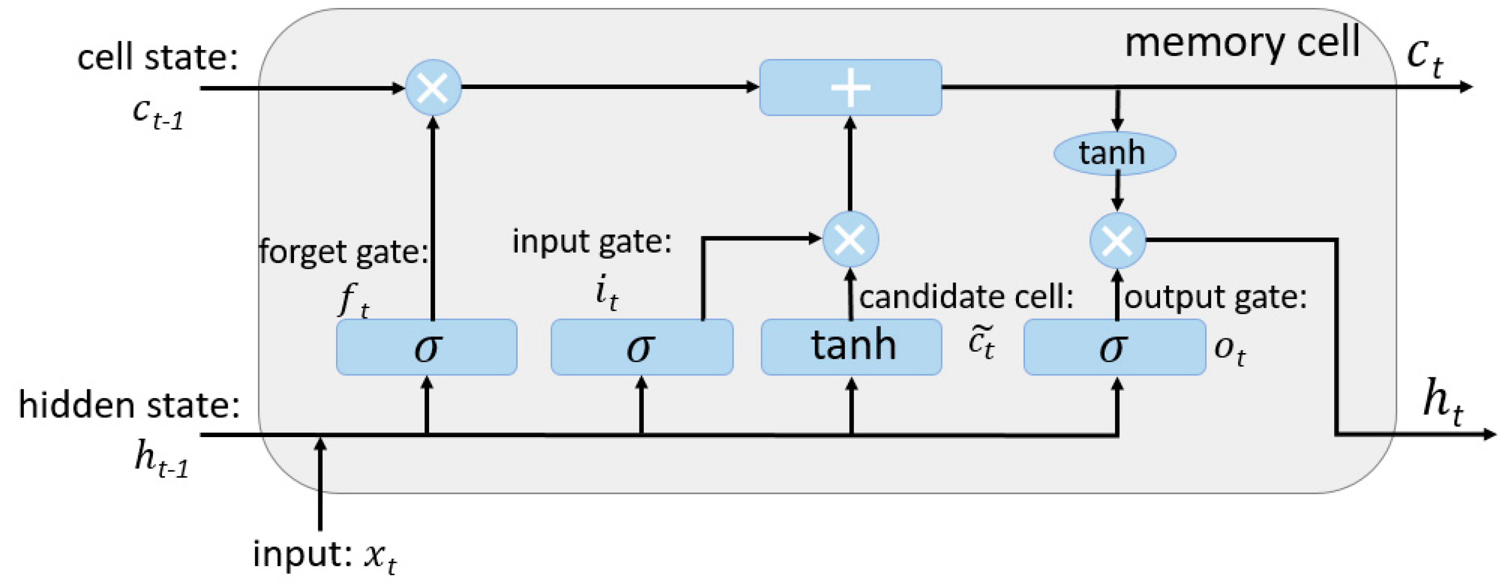
15]. Precipitation is always a kind of typical time-sequential data and varies greatly in time. Recurrent Neural Networks (RNNs) are some of the state-of-the-art deep learning methods in dealing with time series problems [16]. There are many variants of RNNs, such as Long Short-Term Memory (LSTM), which are more stable. They have been used in the field of computer vision, speech recognition, sentiment analysis, finance, self-driving, and natural language processing [17,18,19,20,21,22]. There have been a number of researches that seek to explain the relationships between meteorological indices and precipitation using deep learning [23,24,25,26,27,28]. Concurrent relationships are typically quantified through deep neural networks analyses between precipitation and a range of meteorological indices such as North Atlantic Oscillation (NAO), East Atlantic (EA) Pattern, West Pacific (WP) Pattern, East Atlantic/West Russia Pattern (EA/WR), Polar/Eurasia Pattern (POL), Pacific Decadal Oscillation (PDO), and so on. For example, Yuan et al. predicted the summer precipitation using significantly correlated climate indices by an Artificial Neural Network (ANN) for the Yellow River Basin [26]. Lee et al. developed a late spring–early summer rainfall forecasting model using an Artificial Neural Network (ANN) for the Geum River Basin in South Korea [28]. Hartmann et al. used neural network techniques to predict summer rainfall in the Yangtze River basin. Input variables (predictors) for the neural network are the Southern Oscillation Index (SOI), the East Atlantic/Western Russia (EA/WR) pattern, the Scandinavia (SCA) pattern, the Polar/Eurasia (POL) pattern, and several indices calculated from sea surface temperatures (SST), sea level pressures (SLP), and snow data [23]. However, the meteorological indices they used are global teleconnection patterns, and the approaches are applicable for long-time precipitation prediction and large-scale areas such as a country or a river basin. For a city or smaller area, the short-time precipitation may have a relatively weak relationship with the global teleconnection patterns, so other meteorological variables are needed to predict precipitation.
Some researchers have used the meteorological variables, such as Maximum Temperature, Minimum Temperature, Maximum Relative Humidity, Minimum Relative Humidity, Wind Speed, Sunshine, and so on, to predict the precipitation [29,30,31,32]. Gleason et al. designed the time series and case-crossover model to evaluate associations of precipitation and meteorological factors, such as temperature (daily minimum, maximum, and mean), dew point, relative humidity, sea level pressure, and wind speed (daily maximum and mean) [29]. Poornima et al. presented an Intensified Long Short-Term Memory (Intensified LSTM) using Maximum Temperature, Minimum Temperature, Maximum Relative Humidity, Minimum Relative Humidity, Wind Speed, Sunshine, and Evapotranspiration to predict rainfall [30]. Jinglin et al. applied deep belief networks in weather precipitation forecasting using atmospheric pressure, sea level pressure, wind direction, wind speed, relative humidity, and precipitation [33]. However, they did not consider the contribution of the meteorological variables. The relationships between meteorological variables and precipitation vary with season and location. Not all the meteorological variables have a strong relationship with precipitation, and some of them may have a negative impact on the accuracy of the prediction. Therefore, meteorological variables selection is the key and difficult point to the application of precipitation prediction. However, little research has considered the contribution of the meteorological variables.
In meteorology, precipitation is any product of the condensation of atmospheric water vapor that falls under gravity. So, meteorological variables are potentially useful predictors of precipitation. The main contribution of this study is using the twice screening method to select effective meteorological variables and discard useless or counteractive indicators to predict precipitation by the LSTM model, according to different characteristics of each place. So, the objectives of this study are to: (1) propose a method of selecting available and effective variables to predict precipitation; (2) analyze whether the simulation performance can be improved by inputting refined meteorological variables; (3) compare the simulation capability of the LSTM model with other models (i.e., Autoregressive Moving Average model (ARMA) and Multivariate Adaptive Regression Splines (MARS) as the statistical algorithms and Back-Propagation Neural Network (BPNN), Support Vector Machine (SVM), Genetic Algorithm (GA), and traditional ANN models). The results of this study can provide better understandings of the potential of the LSTM in precipitation simulation applications. In this study, after one-hot encoding and normalizing the meteorological data, the possible candidate variables of meteorological variables are preliminarily determined by circular correlation analysis. Then, the candidate variables are used to construct the LSTM model, and the input variables with the greatest contribution are selected to reconstruct the LSTM model. Finally, the LSTM model with the final selected input variables is used to predict the precipitation and the performance is compared with other classical statistical algorithms and the machine learning algorithms. The result shows that the performance of the LSTM model with particular meteorological variables is better than the classical predictors and the time-consuming and laborious trial–error process is greatly reduced.

2. Overview of Study Area

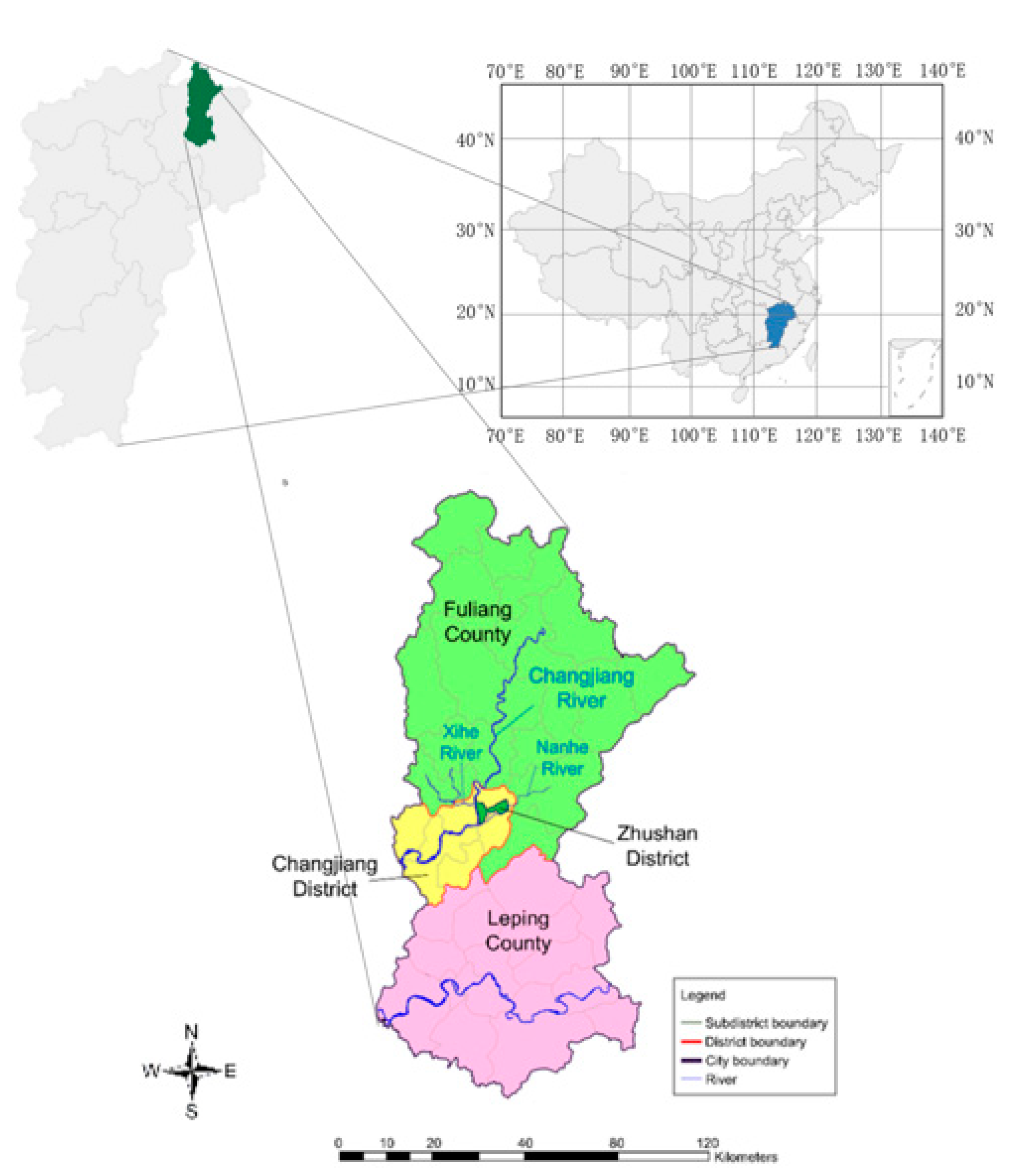
Jingdezhen is a typical small- and medium-sized city in China, with rapid social and economic development, and the population of Jingdezhen is almost 1.67 million. It is located in the northeast of Jiangxi province, and it belongs to the transition zone between the extension of Huangshan Mountain, Huaiyu Mountain, and Poyang Lake Plain (as shown in Figure 1). The city covers an area of 718.93 km2, between 116°57′ E and 117°42′ E and 28°44′ N and 29°56′ N latitude.
Jingdezhen is characterized by a subtropical monsoon climate affected by the East Asian monsoon, with abundant sunshine and rainfall. It has long, humid, and very hot summers, and cool and drier winters with occasional cold snaps. The annual average temperature is 17.36 °C and extreme maximum temperatures of above 40 °C have been recorded, as have extreme minimums below −5 °C. The annual precipitation is 1763.5 mm, and the distributions of precipitation are quite uneven, with about 46% of precipitation occurring in the rainy season (from April to June). The average rainfall is about 200–350 mm in the rainy season, which is extremely prone to flooding. In 2016, the city’s 24-h average rainfall exceeded 300 mm with a return period of 20 years and the maximum flow of the Chengjiang River was 7090 m3/s. The flood caused by the extreme rainfall return period of the main stream of the Chengjiang River was 20 years, and some river sections were 50 years.

3. Results

3.1. Data Sources

The meteorological data was collected from Jingdezhen Meteorology Bureau, Jingdezhen Statistical Yearbook, Jingdezhen Water Resource Bulletin. Statistics were provided by the Jingdezhen Flood Control and Drought Relief Headquarters, which is also responsible for data quality. In this study, the meteorological data of Jingdezhen ranges from 01 January 2008 to 31 December 2018, and 14 observations are available for each day with 3 h intervals. The original data contains temperature (T), dew point temperature (Td), minimum temperature (Tn), maximum temperature (Tx), atmospheric pressure (AP), pressure tendency (PT), relative humidity (RH), wind speed (WS), wind direction (WD), maximum wind speed (WSx), total cloud cover (TCC), height of the lowest clouds (HLC), amount of clouds (AC), and precipitation (PRCP). Table 1 summarizes the meteorological data and provides brief descriptions of each.

3.2. Selecting Meteorological Variables

In meteorology, precipitation is any product of the condensation of atmospheric water vapor that falls under gravity. It is a quasi-periodic phenomenon. So, meteorological variables are potentially useful predictors of precipitation. However, not all the meteorological variables have a strong relationship with precipitation, and some of them may affect the accuracy of the prediction. Therefore, meteorological variables selection is the key and difficult point to the application of the model. Circular cross-correlation (CCC) is a number that describes some characteristics of the relationship between two variables, which are equal-length periodic data [34]. Thus, CCC is employed to solve the meteorological variables selecting problem. The steps of the meteorological variables selecting algorithm are as follows.

3.2.1. Binarizing Categorical Features

The meteorological data can be divided into two categories, one is the categorical data, the other one is numerical data. Because the RNN models cannot operate the categorical data directly, it is necessary to binarizing categorical data. In this study, one-hot encoding can be applied to the integer representation [35]. The one-hot function provides an interface to convert categorical data into a so-called one-hot array, where each unique data is represented as a column in the new array. Each value of a categorical feature is treated as a state. If there are N different values, N is the number of categorical variables, then the categorical feature can be abstracted into N different states. One-hot encoding can ensure that each value can cause only one state to be in the “active state”, that is, only one of the N states has a value of one and all other state bits are zero. For instance, the wind direction is converted into numerical form, the label encoding and one-hot encoding of the wind direction are shown in Table 2 and Table 3, respectively.
After the one-hot encoding of categorical features, the features of each dimension can be regarded as continuous features. So, they can be used in RNN models.

3.2.2. Binarizing Categorical Features

Suppose there are n records of meteorological data and m meteorological variables, and Xij (i = 1, 2, …, n; j = 1, 2, …, m) denotes the value of index j in record i, as described in Equations (1). Due to the difference in indicator values and units, it is necessary to normalize the records.
x i j = X i j X m e a n j X m a x j X m i n j ,
where Xmeanj, Xmaxj, and Xminj are the mean, the maximum, and the minimum index j of all records, respectively, and xij is the normalized value.

3.2.3. Calculating the CCC

Suppose a = {a1, a2, …, an} is the normalized precipitation vector and b = {b1, b2, …, bn} is one of the normalized meteorological vectors. In order to calculate the CCC between precipitation and the meteorological variable, Equation (2) should be employed:
r = i = 1 n 1 j = i + 1 n sin ( a i a j ) sin ( b i b j ) i = 1 n 1 j = i + 1 n sin 2 ( a i a j ) i = 1 n 1 j = i + 1 n sin 2 ( b i b j ) ,
where r is the CCC and n is the number of data records. The absolute value of r takes on values within the interval from zero to one, where zero indicates that there is no relationship between the variables and one represents the strongest association possible. For a positive r, the relationship is positively related, while for a negative r, the variables have a negative relationship.

3.3. Constructing of the LSTM Model Arctecture

Suppose d is the number of selected meteorological variables after identifying the precipitation between each of the other meteorological variables. T is the length of the observed time series. Set the observed time series x = {x1, x2, …, xT} as the input of the LSTM. xt ( t T ) represents the meteorological vector observed at time step t. Then, the dimension of input data equals d. The output of the LSTM is the predicted precipitation data at time step t+1, denoted as y t ^ . The dimension of output data equals 1. The actual rainfall value is denoted as y t . Because the interval between two records is 3 h, the time step is set to 3 h. This means that LSTM can be used to predict the next 3-h of precipitation.
LSTM is a special kind of RNN, capable of learning long-term dependence. It was introduced by Hochreiter and Schmidhuber [36], and was refined and popularized by many people in the following work. The difference between LSTM and RNN is that it adds a “processor”, which is called cell state, to the algorithm to judge whether the information is useful or not. In a cell, three gates are placed, called input gate, forget gate, and output gate, the architecture of the LSTM memory cell is shown in Figure 2.
A network where information enters LSTM can be judged by rules. Only the information that accords with the authentication will be left behind, and the discrepant information is forgotten by the forget gate. The main steps are as follows.
Step 1: The forget gate f t defines what information will be thrown away from the memory, by using a sigmoid layer. The forget state function is defined as in Equation (3):
f t = σ ( W f · x t + W f · h t 1 + b f ) ,
where σ is the sigmoid activation function, W f is the weight vector for f t , x t is the input, h t 1 is the previous hidden state, and b i is the bias for forget gate. It will output a number between zero and one. For each number in the cell state c t 1 , one represents “completely keep this” while zero represents “completely get rid of this.”
Step 2: The input gate i t and the candidate cell C t ˜ both decide what new information will be stored in the cell state. The functions are defined as in Equation (4) and (5):
i t = σ ( W i · x t + W i · h t 1 + b i ) ,
C t ˜ = t a n h ( W C · x t + W C · h t 1 + b C ) ,
where W i and W C are the weight vector for i t and C t , b i , and b C are the bias for i t and C t . The tanh activation function is used to push the values to be between −1 and 1. Then, i t and C t will be combined to create an update to the state, by the formula in Equation (6):
C t = f t c t 1 + i t C t ˜ ,
where C t is the new cell state, so that the network can drop the old information and add the new information.
Step 3: The output gate o t defines what information from the memory is going to be outputted. The functions are defined as in Equation (7) and (8):
o t = σ ( W o · x t + W o · h t 1 + b o ) ,
h t = o t t a n h ( C t ) ,
where W o is the weight vector for o t , b o are the bias for o t . Then, C t is put through the tanh function and multiplied by o t , so that the new cell state and the hidden state are calculated.

3.4. Optimization of the LSTM Model

3.4.1. Performing the LSTM Model

The LSTM model structures were determined using the k-fold Cross-Validation procedure by varying the number of hidden neurons from 2 to 10. The k-fold Cross-Validation procedure has a single parameter called k that refers to the number of groups that a given data sample is to be split into. There is a bias–variance trade-off associated with the choice of k in k-fold Cross-Validation. Empirically, five is the best value of k, as it has shown test error rate estimates that suffer neither from excessively high bias nor from very high variance [37]. The procedure is as follows:
Step 1: Shuffle the dataset randomly.
Step 2: Split the dataset into five groups.
Step 3: For each unique group:
  • Take the group as a hold out or test dataset.
  • Take the remaining groups as a training dataset.
  • Fit the LSTM model on the training dataset and evaluate it on the test dataset.
  • Retain the evaluation score.
Step 4: Summarize the skill of the models using the sample of model evaluation scores.
Therefore, for each hidden neuron, five iterations of the training and validation were performed.

3.4.2. Determining the Input Variables with the Greatest Contribution

The relative contribution of input variables to the output value is a good index to establish the relations between input variables and the output value provided by a Multilayer Perceptron [38]. Garson proposed a method [39], later modified by Goh [40] for determining the relative importance of an input node to a network. The details of the method are given in Equation (9):
Q i k = j = 1 L | w i j v j k | / r = 1 N | w r j | i = 1 N j = 1 L ( | w i j v j k | / r = 1 N | w r j | ) ,
where w i j is the weight between the input unit i and the hidden unit j, v j k is the weight between the hidden unit j and the output unit k, and r = 1 N | w r j | is the sum of the weights between the N input units and the hidden unit j. Q i k represents the percentage of influence of the input variable on the output value. In order to avoid the counteracting influence due to positive and negatives values, all connection weights were given their absolute values in the modified Garson method.

3.4.3. Evaluating the Performance

To systematically examine the performance of different models by statistical error measures and characteristics of precipitation process error, we include results with two widely used prediction error metrics: Symmetric Mean Absolute Percentage Error (SMAPE) [41] and Root Mean Square Error (RMSE) [42].
The Symmetric Mean Absolute Percentage Error, SMAPE, measures the size of the error in percentage terms. It is calculated as the average of the absolute value of the actual and the absolute value of the forecast in the denominator. It is usually defined as in Equation (10):
SMAPE = 100 % n i = 1 n | F i A i | ( | F i | + | A i | ) / 2 ,
where A i is the actual value and F i is the predicted value.
The Root Mean Square Error, RMSE, is used to measure the deviation between the predicted value and the true value. It is the square root of the average of squared errors. The effect of each error on RMSE is proportional to the size of the squared error; thus, larger errors have a disproportionately large effect on RMSE. Consequently, RMSE is sensitive to outliers. It is usually defined as in Equation (11):
RMSE = i = 1 n ( y i y i ^ ) 2 n ,
where y i ^ is the predicted value,   y i is the true value, and n is the size of dataset. Compare the prediction performance of different numbers of hidden neurons and determine the best number of hidden neurons for the model.
Threat Score (TS) is used to evaluate the accuracy and prediction capability of prediction results, which is mainly used in the National Meteorological Center of China [43]. TS1 is used to represent the proportions of samples which are forecasted correctly, including accurate prediction of precipitation or no precipitation. TS2 is used to represent the proportions of samples which can only accurately predict precipitation. TS3 is the average value of TS1 and TS2. Detailed descriptions of the TS score are defined as in Equation (12), (13) and (14):
T S 1 = N 1 + N 2 N 1 + N 2 + N 3 + N 4 ,
T S 2 = N 1 N 1 + N 3 + N 4 ,
T S 3 = T S 1 + T S 2 2 ,
where N1 represents the number of samples to predict the correct precipitation, N2 represents the correct number of samples for forecasting no precipitation, N3 represents the number of samples that predict no precipitation but actually rain, and N4 represents the number of samples that predict precipitation but do not actually have precipitation.

4. Results and Discussion

4.1. Experimental Setup

Because the distributions of precipitation in Jingdezhen are quite uneven, 46% of precipitation occurred in the rainy season (from April to June) and a great deal of observed precipitation is equal to zero in the non-rainy season. To balance the positive and negative data, the data from April to June every year, total 192,192 records, are selected to train, validate, and test the model by five-fold Cross-Validation.
In this study, the interval of the meteorological data is 3 h. The data in the first 21 h are used to predict the data in the last three hours each day. The “many to one” LSTM model is used, so the size of the input is seven and the output length is one. The number of neurons affects the learning capacity of the network. Generally, more neurons would be able to learn more structure from the problem at the cost of longer training time. Then, we can objectively compare the impact of increasing the number of neurons while keeping all other network configurations fixed. We repeat each experiment 30 times and compare performance with the number of neurons ranging from 2 to 10.
The hyperparameters used to train this model were: epoch was 100, each epoch had 30 steps, a total of 3000 steps; the learning rate was 0.02; the batch size was 7, and every 50 steps, the loss value will be recorded once. We performed all the training and computation in the TensorFlow2.0 computational framework using an NVIDIA GeForce GTX 1070 and NVIDIA UNIX x86_64 Kernel Module 418 on a discrete server running a Linux system (Ubuntu18.04.3) (Canonical Group Limited, London, UK) with an Intel(R) Core(TM) i7-8700 CPU @ 3.20 GH (Intel Corporation, Santa Clara, CA, USA).

4.2. Meteorological Variables Analysis

According to the weather system, precipitation is a major component of the water cycle. Considering the actual situation of Jingdezhen, the precipitation predictor variables we choose are closely related to the water cycle. The predictor variables are temperature (T), dew point temperature (Td), minimum temperature (Tn), maximum temperature (Tx), atmospheric pressure (AP), pressure tendency (PT), relative humidity (RH), wind speed (WS), wind direction (WD), maximum wind speed (WSx), total cloud cover (TCC), height of the lowest clouds (HLC), and amount of clouds (AC). Because the distributions of precipitation in Jingdezhen are quite uneven, 46% of precipitation occurred in the rainy season (from April to June) and a great deal of observed precipitation is equal to zero in the non-rainy season. To balance the positive and negative data, the data from April to June every year are selected to train the model.
After one-hot encoding and normalizing the meteorological variables and historical precipitation data, the CCC between precipitation and each of the meteorological variables were calculated (see Table 4). As shown from the results, it is evident that meteorological variables are potentially useful predictors of precipitation. A maximum negative correlation of -0.4768 was achieved for PT and a positive maximum correlation of 0.4475 is obtained for Td. However, the absolute value of CCC between precipitation and Tn, Tx, WD, and WSx is less than 0.1. So, Tn, Tx, WD, and WSx are ignored. The highly correlated nine meteorological variables, including T, Td, AP, PT, RH, WS, TCC, HLC, and AC, were selected as inputs for the LSTM model.

4.3. Preliminary LSTM Model for Precipitation Prediction

The optimal LSTM model structure with the selected nine input variables, was determined using the five-fold Cross-Validation procedure by varying the number of hidden neurons from 2 to 10. For each hidden neuron, five iterations of the training and validation were performed. The whole dataset of training and validation was used to train the selected models, and the weights for these trained structures were saved and the networks were evaluated for testing.
The average RMSE, SMAPE, and TS scores between the actual precipitation and the predicted precipitation measured using the LSTM model with the selected nine input variables are presented in Table 5. The results show that the performance of the model with different numbers of hidden neurons was not significantly different. The results also show that a larger number of hidden neurons did not always lead to better performance. In the training part, the SMAPE values ranged from 16.28% to 19.63%, and RMSE values ranged from 46.45 mm to 51.31 mm. In the validation part, the SMAPE values ranged from 18.01% to 20.64%, and RMSE values ranged from 49.61 mm to 54.26 mm. In the testing part, the SMAPE values ranged from 18.16% to 21.74%, and RMSE values ranged from 47.61 mm to 54.71 mm. The TS1 score values ranged from 0.74 to 0.82, the TS2 score values ranged from 0.55 to 0.61, and the TS3 score values ranged from 0.66 to 0.71. The accuracy of the results is acceptable. Based on the minimum error in five-fold Cross-Validation, the structure with six hidden neurons in the LSTM model was considered the best, which are denoted as LSTM (9,6,1).
Compared with the average RMSE, SMAPE, and TS score of the LSTM model with all 13 input variables (see Table 6), only when the number of hidden neurons is three or eight, the average RMSE and SMAPE of the LSTM model with the selected nine input variables are worse. Except that the number of hidden neurons is three or eight, the average RMSE and SMAPE are better. The structure with eight hidden neurons in the LSTM model with all 13 input variables was considered the best, which are denoted as LSTM (13,8,1).
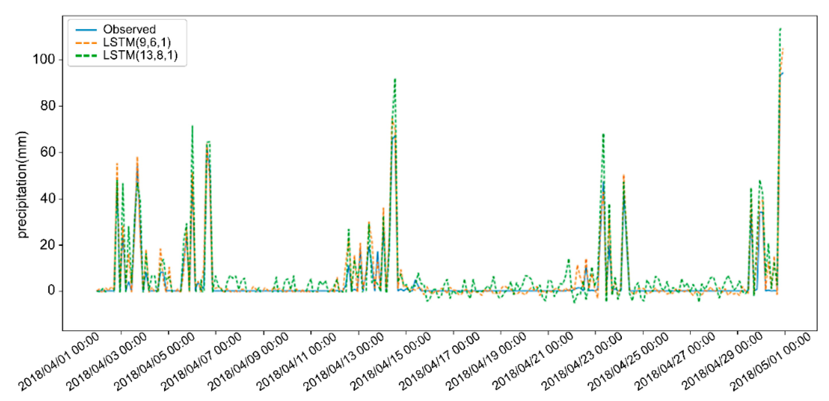
Figure 3 shows the precipitation prediction results for 3 h LSTM (9,6,1) and LSTM (13,8,1) in April 2018, which is the month with the largest precipitation in 2018. The predicted result LSTM (9,6,1) is better than LSTM (13,8,1). Therefore, after selecting meteorological variables by circular cross-correlation, the LSTM model with the selected nine input variables can perform better.

4.4. Quantification of Relative Importance of Input Variables

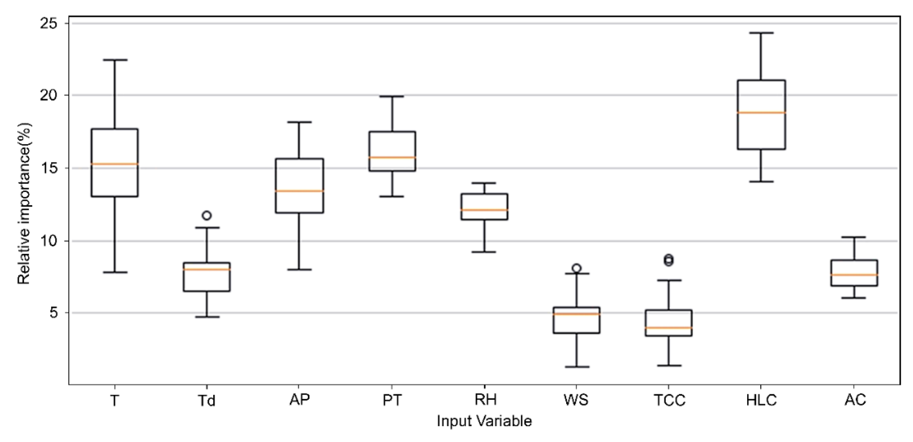
The relative contribution of input variables to the output value was quantified using the modified Garson’s weight method. Figure 4 shows the relative importance of the nine variables obtained from Garson’s connection weights method in the form of a box plot. According to the different random initial weights, great changes in the importance values will be observed. Results show that in the LSTM (9,6,1) model, HLC shows the strongest relationship with predicted precipitation and its contribution of median value is 18.24%. TCC shows the weakest relationships; the contribution of the median value is less than 5%. There are several abnormal values, but the proportion is very low, so they are ignored. The top five important predictors are HLC, PT, T, AP, and RH.
We have talked about the general relative importance of input variables of the LSTM model in the above study. As we can see, HLC, PT, T, AP, and RH are the most important predictors, which always have a relative importance above 10%. WS and TCC are the least important predictors.
The urban heat island warms cities from 0.6 to 5.6 °C above surrounding suburbs and rural areas. This extra heat leads to greater upward motion, greater change of humidity, and atmospheric pressure, which can induce additional shower and thunderstorm activity [44]. The study area, Jingdezhen City, is a fast-developing urbanized area situated at the transition zone between the Yellow Mountain, extension ranges of the Huaiyu Mountain, and the Poyang Lake Plain. The urban heat island also is a common phenomenon in Jingdezhen, and the local temperature, humidity, air convection, and other factors on the urban surface in Jingdezhen have changed. Therefore, local meteorology in Jingdezhen has been affected by urban heat island, the rates of precipitation have also been greatly affected. So, the height of the lowest clouds, temperature, atmospheric pressure, and humidity have a great impact on precipitation. However, Jingdezhen is surrounded by mountains, and the wind speed has a relatively small impact on precipitation. The quantification of the relative importance of input variables, analyzed by the LSTM model, is also good proof of this phenomenon. So, HLC, PT, T, AP, and H are selected to reconstruct the LSTM model.

4.5. Best LSTM Model for Precipitation Prediction

The optimal LSTM model structure with five input variables (HLC, PT, T, AP, and RH) was determined by varying the number of hidden neurons from 2 to 10. Table 7 shows the training, validation, and testing results for the LSTM structures. As the number of hidden neurons increased, the trends of the change of the RMSE, SMAPE, and TS score decreased generally and reached a minimum value when the number of hidden neurons was five, but after five hidden neurons they increased. In the training part, the SMAPE values ranged from 14.16% to 15.69%, and RMSE values ranged from 42.28 mm to 43.49 mm. In the validation part, the SMAPE values ranged from 14.28% to 15.83%, and RMSE values ranged from 42.03 mm to 43.27 mm. In the testing part, the SMAPE values ranged from 14.17% to 16.06%, and RMSE values ranged from 41.72 mm to 43.68mm. The TS1 score values ranged from 0.82 to 0.89, the TS2 score values ranged from 0.57 to 0.63, and the TS3 score values ranged from 0.70 to 0.76. The prediction results are better than the LSTM model structure with the nine input variables. When the number of hidden neurons is five, the LSTM model structure with five input variables (HLC, PT, T, AP, and RH) performed the best, are denoted as LSTM (5,5,1).
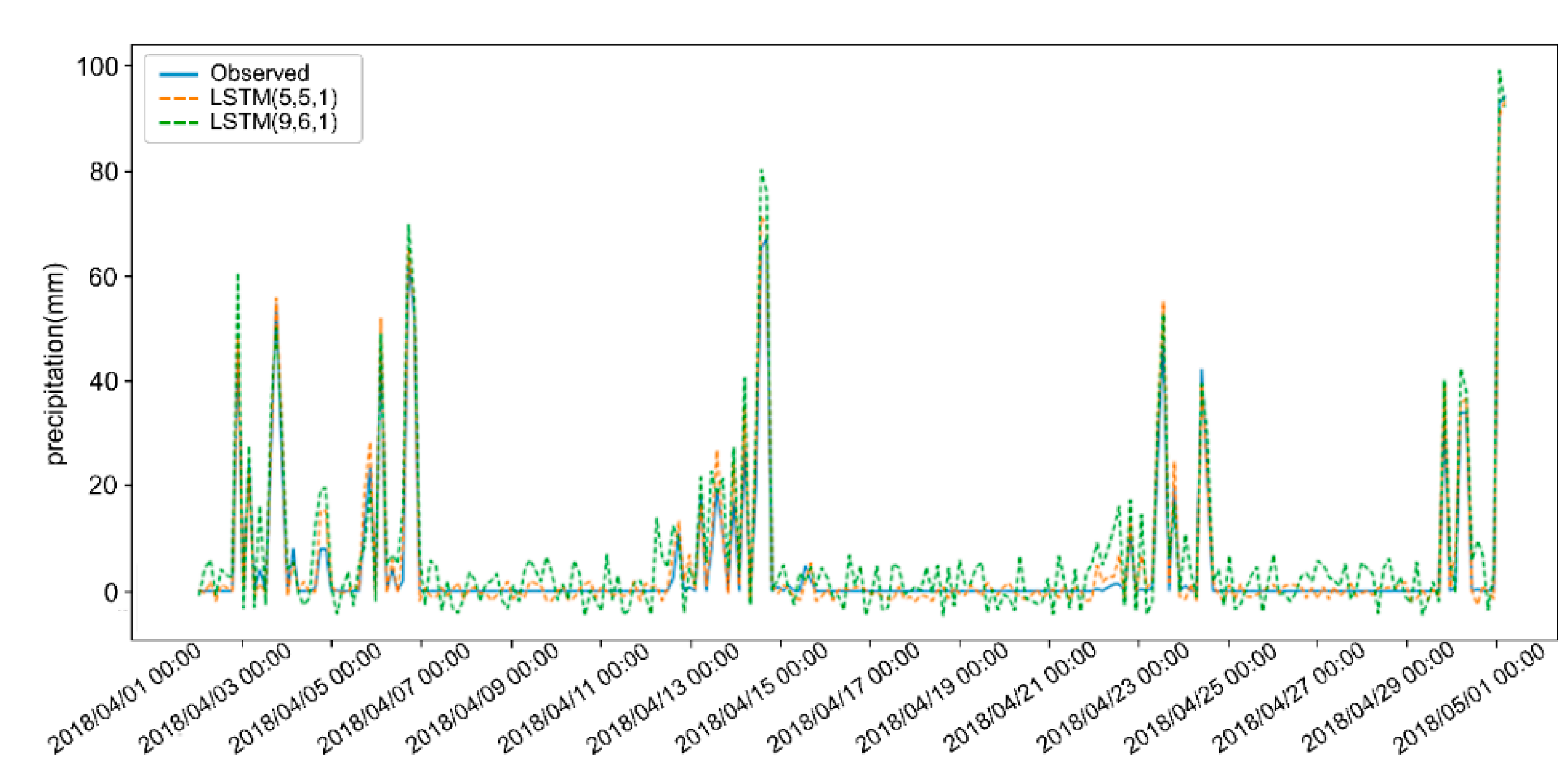
The precipitation prediction results by LSTM (5,5,1) and LSTM (9,6,1) for 3 h in April, 2018 are shown in Figure 5. The predicted result LSTM (5,5,1) is evidently better than LSTM (9,6,1). Therefore, after further refining meteorological variables by the relative importance of input variables, the LSTM model can perform better.
In addition, we select the Autoregressive Moving Average model (ARMA) and Multivariate Adaptive Regression Splines (MARS) as the statistical algorithms and Back-Propagation Neural Network (BPNN), Support Vector Machine (SVM), and Genetic Algorithm (GA) as the machine learning algorithms for performance comparison. The test data set is from April to June 2018, which was a noted rainy season in 2018. The prediction performances are shown in Table 8.
In comparison with the predictors, the performances of ARMA and MARS are evidently worse than BPNN, SVM, and GA. The performance of BPNN is better than SVM and GA, of which the performances are quite near. LSTM has better performance than the other classical machine learning models. It indicates that traditional statistics algorithms predict the precipitation only based on the previous meteorological data without taking the rapid changes caused by human activities and climate change into account. Classical machine learning algorithms take recent changes into account, but they make no discrimination between the long-term and short-term data. Therefore, they cannot predict the precipitation with great accuracy. However, LSTM can take advantage of all the historical data and recent changes, and it can balance the long-term and short-term data with larger weights for short-term data and less weight for long-term data. So, this study implies that with particular meteorological variables, LSTM could also outperform the statistics algorithms and classical machine learning predictors.

4.6. Scope of Application

Topography is one of the important factors affecting precipitation and its distribution. In mountainous environments, precipitation will change dramatically with the height of the mountain slopes over short distances. The meteorological parameters can change quickly over a short time and space scales in rough topography, among which the temperature changes most acutely [45]. In cold climatic regions, atmospheric motions and thermodynamics also have a great impact on precipitation [46]. So, rough topography and extreme climate have a great impact on the accuracy of the provided approach.
The approach provided in this study is mainly applicable to plains with a small area, where meteorological elements change gently. In mountainous environments such as Tibet or high latitude areas, because meteorological conditions change rapidly, this approach is not applicable at present. In a future study, the digital elevation model (DEM) will be considered as the main factor affecting precipitation intensity. More sensors need to be constructed to record more data. For every dataset recorded by the sensors, the provided approach can be used to predict the precipitation. The precipitation results can be distributed to different areas by the interpolation method to expand the prediction scale.
In recent years, the application of artificial intelligence (AI) in the field of meteorology has shown explosive growth and makes many achievements. However, the prediction quality of AI techniques is limited by the quality of input data. Most AI technologies are similar to “black box”, which works well under normal circumstances, but may fail in extreme situations. In order to achieve better results, it is necessary to strengthen the research and development of high-quality and long sequence meteorological training datasets, such as providing long history and consistent statistical characteristics of model data, sorting out and developing high-resolution observation, and analyzing data for training and testing.

5. Conclusions

In this study, five relative importance of input variables were selected to predict the precipitation by LSTM in Jingdezhen City, China. For this purpose, after identifying the circular cross-correlation coefficient between meteorological variables and precipitation amount in Jingdezhen, nine meteorological variables, which are T, Td, AP, PT, H, WS, TCC, HLC, and AC, were selected to construct the LSTM model. Then, the selected meteorological variables were refined by the relative importance of input variables. Finally, the LSTM model with HLC, PT, T, AP, and RH as input variables was used to predict the precipitation and the performance is compared with other classical statistical algorithms and the machine learning algorithms. The main conclusions are the following:
  • The quantification of the contribution of the variable relative importance was able to improve the accuracy of predicting precipitation by removing some input variables that show a weak correlation. The LSTM model can predict precipitation well with the help of the circular cross-correlation analysis and the quantification of variable importance.
  • The LSTM model’s performance with different numbers of hidden neurons was not significantly different. The results show that a large number of hidden neurons did not always lead to better performance. The best LSTM (5,5,1) model showed satisfactory prediction performance with RMSE values of 42.28 mm, 42.03 mm, and 41.72 mm, and SMAPE values of 14.19%, 14.28%, and 14.17% for the training, validation, and testing data sets, respectively.
  • HLC, PT, T, AP, and RH are the most important predictors for precipitation in Jingdezhen City. The optimal model predicted higher values of precipitation to be acceptable, but it needs enough meteorological data. Future studies need to be carried out to improve the models to predict the precipitation in rural areas where there is less data.
In comparison with the studies on precipitation prediction, the approach provided in this study can select different meteorological variables to optimize the precipitation prediction results according to the characteristics of different cities. In conclusion, this study revealed the possibility of precipitation predicting using LSTM and meteorological variables in advance for the study region. Good prediction of the precipitation amount could allow for the more flexible decision-making in Jingdezhen City and provide sufficient time to prepare strategies against potential flood damage. The LSTM model with particular input variables can be considered a data-driven tool to predict precipitation.

Author Contributions

All authors have read and agree to the published version of the manuscript. Conceptualization, J.K.; methodology, J.K. and Z.Q.; formal analysis, F.Y.; resources, Z.W. and T.Q.; data curation, T.Q.; Writing—original draft, J.K.; writing—review & editing, J.H. and F.Y.; visualization, J.K.; project administration, H.W.

Funding

This work was supported by the National Natural Science Foundation of China (Grant No. 91846203, 51861125101), the Fundamental Research Funds for the Central Universities (Grant No. 2017B728X14), and the Research Innovation Program for College Graduates of Jiangsu Province (Grant No. KYZZ16_0263, KYCX17_0517).

Acknowledgments

We would like to express our gratitude to the Jingdezhen Meteorology Bureau and Jingdezhen Flood Control and Drought Relief Headquarters for the support to carry out the study. Finally, we thank the China Scholarship Council for funding us to do research in the University of Florida.

Conflicts of Interest

The authors declare that there is no conflicts of interests regarding the publication of this paper.

References

  1. Kucera, P.A.; Ebert, E.E.; Turk, F.J.; Levizzani, V.; Kirschbaum, D.; Tapiador, F.J.; Loew, A.; Borsche, M. Precipitation from Space: Advancing Earth System Science. Bull. Am. Meteorol. Soc. 2013, 94, 365–375. [Google Scholar] [CrossRef]
  2. Wu, H.; Adler, R.F.; Hong, Y.; Tian, Y.D.; Policelli, F. Evaluation of Global Flood Detection Using Satellite-Based Rainfall and a Hydrologic Model. J. Hydrometeorol. 2012, 13, 1268–1284. [Google Scholar] [CrossRef]
  3. Pasaribu, Y.P.; Fitrianti, H.; Suryani, D.R. Rainfall Forecast of Merauke Using Autoregressive Integrated Moving Average Model. E3S Web Conf. 2018, 73, 12010. [Google Scholar]
  4. Deo, R.C.; Samui, P.; Kim, D. Estimation of monthly evaporative loss using relevance vector machine, extreme learning machine and multivariate adaptive regression spline models. Stoch. Environ. Res. Risk Assess. 2015, 30, 1769–1784. [Google Scholar] [CrossRef]
  5. Chiang, Y.-M.; Chang, L.-C.; Jou, B.J.D.; Lin, P.-F. Dynamic ANN for precipitation estimation and forecasting from radar observations. J. Hydrol. 2007, 334, 250–261. [Google Scholar] [CrossRef]
  6. Deo, R.C.; Wen, X.; Qi, F. A wavelet-coupled support vector machine model for forecasting global incident solar radiation using limited meteorological dataset. Appl. Energy 2016, 168, 568–593. [Google Scholar] [CrossRef]
  7. Rahman, M.; Islam, A.H.M.S.; Nadvi, S.Y.M.; Rahman, R.M. Comparative study of ANFIS and ARIMA model for weather forecasting in Dhaka. In Proceedings of the 2013 International Conference on Informatics, Electronics and Vision (ICIEV), Dhaka, Bangladesh, 17–18 May 2013. [Google Scholar]
  8. Chen, K.; Liu, J.; Guo, S.X.; Chen, J.S.; Liu, P.; Qian, J.; Chen, H.J.; Sun, B. Short-Term Precipitation Occurrence Prediction for Strong Convective Weather Using Fy2-G Satellite Data: A Case Study of Shenzhen, South China. In Proceedings of the XXIII ISPRS Congress, Commission VI, Prague, Czech Republic, 12–19 July 2016; Volume 41, pp. 215–219. [Google Scholar] [CrossRef]
  9. Guhathakurta, P.; Kumar Kowar, M.; Karmakar, S.; Shrivastava, G. Application of Artificial Neural Networks in Weather Forecasting: A Comprehensive Literature Review. Int. J. Comput. Appl. 2012, 51, 17–29. [Google Scholar] [CrossRef]
  10. Pasini, A.; Langone, R. Attribution of Precipitation Changes on a Regional Scale by Neural Network Modeling: A Case Study. Water 2010, 2, 321–332. [Google Scholar] [CrossRef] [Green Version]
  11. Nasseri, M.; Asghari, K.; Abedini, M.J. Optimized scenario for rainfall forecasting using genetic algorithm coupled with artificial neural network. Expert Syst. Appl. 2008, 35, 1415–1421. [Google Scholar] [CrossRef]
  12. Hosseini, S.M.; Mahjouri, N. Integrating Support Vector Regression and a geomorphologic Artificial Neural Network for daily rainfall-runoff modeling. Appl. Soft Comput. 2016, 38, 329–345. [Google Scholar] [CrossRef]
  13. LeCun, Y.; Bengio, Y.; Hinton, G. Deep learning. Nature 2015, 521, 436–444. [Google Scholar] [CrossRef] [PubMed]
  14. Schmidhuber, J. Deep learning in neural networks: An overview. Neural Netw. 2015, 61, 85–117. [Google Scholar] [CrossRef] [PubMed] [Green Version]
  15. Glorot, X.; Bordes, A.; Bengio, Y. Domain Adaptation for Large-Scale Sentiment Classification: A Deep Learning Approach. In Proceedings of the International Conference on International Conference on Machine Learning, Bellevue, Washington, DC, USA, 28 June–2 July 2011; pp. 97–110. [Google Scholar]
  16. Shi, H.; Xu, M.; Li, R. Deep Learning for Household Load Forecasting—A Novel Pooling Deep RNN. IEEE Trans. Smart Grid 2017, 9, 5271–5280. [Google Scholar] [CrossRef]
  17. Jafari-Marandi, R.; Khanzadeh, M.; Smith, B.; Bian, L. Self-Organizing and Error Driven (SOED) artificial neural network for smarter classifications. J. Comput. Des. Eng. 2017, 4, 282–304. [Google Scholar] [CrossRef]
  18. Kendall, A.; Gal, Y. What Uncertainties Do We Need in Bayesian Deep Learning for Computer Vision. In Advances in Neural Information Processing Systems 30; Guyon, I., Luxburg, U.V., Bengio, S., Wallach, H., Fergus, R., Vishwanathan, S., Garnett, R., Eds.; Neural Information Processing Systems (Nips): San Diego, CA, USA, 2017; Volume 30. [Google Scholar]
  19. Huang, Z.; Siniscalchi, S.M.; Lee, C.H. A unified approach to transfer learning of deep neural networks with applications to speaker adaptation in automatic speech recognition. Neurocomputing 2016, 218, 448–459. [Google Scholar] [CrossRef]
  20. Tang, D.; Qin, B.; Liu, T. Deep learning for sentiment analysis: Successful approaches and future challenges. Wiley Interdiscip. Rev. Data Min. Knowl. Discov. 2015, 5, 292–303. [Google Scholar] [CrossRef]
  21. Heaton, J.B.; Polson, N.G.; Witte, J.H. Deep learning for finance: Deep portfolios. Appl. Stoch. Model. Bus. Ind. 2016, 33, 3–12. [Google Scholar] [CrossRef]
  22. Donahue, J.; Hendricks, L.A.; Rohrbach, M.; Venugopalan, S.; Guadarrama, S.; Saenko, K.; Darrell, T. Long-Term Recurrent Convolutional Networks for Visual Recognition and Description. IEEE Trans. Pattern Anal. Mach. Intell. 2017, 39, 677–691. [Google Scholar] [CrossRef] [PubMed]
  23. Hartmann, H.; Becker, S.; King, L. Predicting summer rainfall in the Yangtze River basin with neural networks. Int. J. Clim. 2008, 28, 925–936. [Google Scholar] [CrossRef]
  24. Miao, Q.; Pan, B.; Hao, W.; Hsu, K.-L.; Sorooshian, S. Improving Monsoon Precipitation Prediction Using Combined Convolutional and Long Short Term Memory Neural Network. Water 2019, 11, 977. [Google Scholar] [CrossRef] [Green Version]
  25. Schepen, A.; Wang, Q.; Robertson, D. Evidence for Using Lagged Climate Indices to Forecast Australian Seasonal Rainfall. J. Clim. 2012, 25, 1230–1246. [Google Scholar] [CrossRef]
  26. Yuan, F.; Berndtsson, R.; Uvo, C.B.; Zhang, L.; Jiang, P. Summer precipitation prediction in the source region of the Yellow River using climate indices. Hydrol. Res. 2015, 47, 847–856. [Google Scholar] [CrossRef] [Green Version]
  27. Grotjahn, R.; Black, R.; Leung, R.; Wehner, M.; Barlow, M.; Bosilovich, M.; Gershunov, A.; Gutowski, W.J.; Gyakum, J.R.; Katz, R.; et al. North American extreme temperature events and related large scale meteorological patterns: A review of statistical methods, dynamics, modeling, and trends. Clim. Dyn. 2015, 46, 1151–1184. [Google Scholar] [CrossRef] [Green Version]
  28. Lee, J.; Kim, C.; Lee, J.E.; Kim, N.W.; Kim, H. Application of Artificial Neural Networks to Rainfall Forecasting in the Geum River Basin, Korea. Water 2018, 10, 1448. [Google Scholar] [CrossRef] [Green Version]
  29. Gleason, J.A.; Kratz, N.R.; Greeley, R.D.; Fagliano, J.A. Under the Weather: Legionellosis and Meteorological Factors. EcoHealth 2016, 13, 293–302. [Google Scholar] [CrossRef]
  30. Poornima, S.; Pushpalatha, M. Prediction of Rainfall Using Intensified LSTM Based Recurrent Neural Network with Weighted Linear Units. Atmosphere 2019, 10, 18. [Google Scholar] [CrossRef] [Green Version]
  31. Xingjian, S.; Chen, Z.; Wang, H.; Yeung, D.-Y.; Wong, W.-K.; Woo, W.-C. Convolutional LSTM Network: A Machine Learning Approach for Precipitation Nowcasting. In Proceedings of the Advances in Neural Information Processing Systems, Montreal, QC, Canada, 7–12 December 2015; pp. 802–810. [Google Scholar]
  32. Asanjan, A.A.; Yang, T.; Hsu, K.; Sorooshian, S.; Lin, J.; Peng, Q. Short-Term Precipitation Forecast Based on the PERSIANN System and LSTM Recurrent Neural Networks. J. Geophys. Res. Atmos. 2018, 123, 12543–12563. [Google Scholar]
  33. Du, J.; Liu, Y.; Liu, Z. Study of Precipitation Forecast Based on Deep Belief Networks. Algorithms 2018, 11, 132. [Google Scholar] [CrossRef] [Green Version]
  34. Fisher, N.I.; Lee, A.J. A Correlation Coefficient for Circular Data. Biometrika 1983, 70. [Google Scholar] [CrossRef]
  35. Matsunaga, Y. Accelerating SAT-Based Boolean Matching for Heterogeneous FPGAs Using One-Hot Encoding and CEGAR Technique. In Proceedings of the 2015 20th Asia and South Pacific Design Automation Conference, Chiba, Japan, 22 January 2015; pp. 255–260. [Google Scholar]
  36. Hochreiter, S.; Schmidhuber, J. Long short-term memory. Neural Comput. 1997, 9, 1735–1780. [Google Scholar] [CrossRef]
  37. James, G.; Witten, D.; Hastie, T.; Tibshirani, R. An Introduction to Statistical Learning: With Applications in R; Springer: New York, NY, USA, 2013. [Google Scholar]
  38. De Ona, J.; Garrido, C. Extracting the contribution of independent variables in neural network models: A new approach to handle instability. Neural Comput. Appl. 2014, 25, 859–869. [Google Scholar] [CrossRef]
  39. Garson, D.G. Interpreting neural network connection weights. Artif. Intell. Expert 1991, 6, 47–51. [Google Scholar] [CrossRef]
  40. Goh, A.T.C. Back-propagation neural networks for modeling complex systems. Artif. Intell. Eng. 1995, 9, 143–151. [Google Scholar] [CrossRef]
  41. Lam, K.F.; Mui, H.W.; Yuen, H.K. A note on minimizing absolute percentage error in combined forecasts. Comput. Oper. Res. 2001, 28, 1141–1147. [Google Scholar] [CrossRef]
  42. Chai, T.; Draxler, R.R. Root mean square error (RMSE) or mean absolute error (MAE)?—Arguments against avoiding RMSE in the literature. Geosci. Model Dev. 2014, 7, 1247–1250. [Google Scholar] [CrossRef] [Green Version]
  43. Zhang, P.; Jia, Y.; Gao, J.; Song, W.; Leung, H.K.N. Short-term Rainfall Forecasting Using Multi-layer Perceptron. IEEE Trans. Big Data 2018. [Google Scholar] [CrossRef]
  44. Estoque, R.C.; Murayama, Y.; Myint, S.W. Effects of landscape composition and pattern on land surface temperature: An urban heat island study in the megacities of Southeast Asia. Sci. Total Environ. 2017, 577, 349–359. [Google Scholar] [CrossRef]
  45. Gultepe, I.; Isaac, G.A.; Joe, P.; Kucera, P.A.; Theriault, J.M.; Fisico, T. Roundhouse (RND) Mountain Top Research Site: Measurements and Uncertainties for Winter Alpine Weather Conditions. Pure Appl. Geophys. 2014, 171, 59–85. [Google Scholar] [CrossRef]
  46. Gultepe, I.; Rabin, R.; Ware, R.; Pavolonis, M. Light Snow Precipitation and Effects on Weather and Climate. In Adv Geophys; Nielsen, L., Ed.; Elsevier Academic Press Inc: San Diego, CA, USA, 2016; Volume 57, pp. 147–210. [Google Scholar]
Figure 1. Geographic location of the study area.
Atmosphere 11 00246 g001
Figure 2. The architecture of the Long Short-Term Memory (LSTM) memory cell.
Atmosphere 11 00246 g002
Figure 3. Three-hour precipitation predictions by LSTM (9,6,1) and LSTM (13,8,1).
Atmosphere 11 00246 g003
Figure 4. Relative importance of input variables in the LSTM model.
Atmosphere 11 00246 g004
Figure 5. Three-hour precipitation predictions by LSTM (5,5,1) and LSTM (9,6,1).
Atmosphere 11 00246 g005
Table 1. Summarizes the meteorological data.
Meteorological VariableDescriptionUnitType
TAir temperature at 2 m height above the earth’s surface°CNumerical
TdDewpoint temperature at a height of 2 m above the earth’s surface°CNumerical
TnMinimum air temperature during the past period (not exceeding 12 h)°CNumerical
TxMaximum air temperature during the past period (not exceeding 12 h)°CNumerical
APAtmospheric pressure at weather station levelmmHgNumerical
PTChanges in atmospheric pressure over the last three hoursmmHgNumerical
RHRelative humidity at a height of 2 m above the earth’s surface%Numerical
WSMean wind speed at a height of 10–12 m above the earth’s surface over a 10 min period immediately preceding the observationm/sNumerical
WDMean wind direction at a height of 10–12 m above the earth’s surface over a 10 min period immediately preceding the observation-Categorical
WSxMaximum wind speed at a height of 10–12 m above the earth’s surface over a 10 min period immediately preceding the observationm/sNumerical
TCCTotal cloud cover-Categorical
HLCHeight of the base of the lowest cloudsmCategorical
ACAmount of all the clouds-Categorical
PRCPAmount of precipitationmmNumerical
Table 2. The label encoding of the wind direction.
Wind DirectionLabel Encoding
East1
West2
South3
North4
Southeast5
Southwest6
Northeast7
Northwest8
Table 3. The one-hot encoding of the wind direction.
EastWestSouthNorthSoutheastSouthwestNortheastNorthwestOne-Hot Encoding
1000000010000000
0100000001000000
0010000000100000
0001000000010000
0000100000001000
0000010000000100
0000001000000010
0000000100000001
Table 4. Selected meteorological variables and the circular cross-correlation value.
Meteorological VariableCircular Cross-Correlation
T0.2363
Td0.4475
Tn0.0853
Tx0.0369
AP0.1835
PT−0.4768
RH0.2176
WS0.1867
WD−0.0163
WSx0.0932
TCC0.2841
HLC−0.3548
AC0.1294
Table 5. The performance for training, validation, and testing parts of the LSTM model with selected nine input variables.
Number of Hidden NeuronsRMSE (mm)SMAPE (%)TS
TrainingValidationTestingTrainingValidationTestingTS1TS2TS3
246.4549.9548.2617.4919.4819.370.820.580.70
349.5154.2653.5117.4920.0521.740.790.590.69
450.2351.3354.6417.3020.3820.960.770.550.66
551.3153.9854.2716.9918.8120.280.750.560.66
648.1949.6147.6116.2818.0118.360.810.600.71
750.4351.2953.2316.9519.5218.690.740.610.68
848.9552.2754.7117.4820.6418.160.800.590.70
950.2353.6254.3716.3020.6318.700.770.600.69
1049.7151.9154.7119.6318.6520.640.790.570.68
Table 6. The performance for training, validation, and testing parts of the LSTM model with all 13 input variables.
Number of Hidden NeuronsRMSE (mm)SMAPE (%)TS
TrainingValidationTestingTrainingValidationTestingTS1TS2TS3
249.2349.8950.3917.9719.6220.050.770.570.67
348.9250.8251.0817.5719.0119.430.790.530.66
453.5152.3854.1619.0521.8421.540.680.510.60
552.4856.0954.8818.2418.9520.350.700.490.60
650.6251.1350.1819.9720.5619.940.750.550.65
749.3249.3550.4118.8419.0319.710.770.550.66
848.3649.7648.8917.5118.6118.650.800.590.70
953.6253.4954.7120.2020.9421.450.650.520.59
1053.7352.7654.0421.4219.8520.6470.680.500.59
Table 7. The performance for training, validation, and testing parts of the LSTM model with five input variables (height of the lowest clouds (HLC), pressure tendency (PT), temperature (T), atmospheric pressure (AP), and relative humidity (RH)).
Number of Hidden NeuronsRMSE (mm)SMAPE (%)TS
TrainingValidationTestingTrainingValidationTestingTS1TS2TS3
243.2543.2743.3815.6915.8316.060.820.590.71
343.2543.1543.1015.9115.7515.240.830.580.71
442.9343.1042.9215.6015.5315.660.850.610.73
542.2842.0341.7214.1914.2814.170.870.610.74
642.3942.2541.9614.1614.5714.630.890.630.76
742.5542.1842.9315.4014.6814.650.880.630.76
842.4442.9343.0315.3214.9914.930.880.610.75
943.0442.9942.9415.2614.9115.650.850.600.73
1043.4942.7243.6815.0515.4515.300.820.570.70
Table 8. Three-hour prediction performance based on the best LSTM model and five other models.
ModelRMSE (mm)SMAPE (%)TS1TS2TS3
ARMA55.7322.560.730.450.59
MARS53.4623.350.710.470.59
BPNN43.0020.390.810.540.68
SVM47.4919.180.760.490.53
GA42.9418.800.800.550.68
LSTM41.8415.170.870.610.74

