Abstract
Predicting the response of wind farms to changing flow conditions is necessary for optimal design and operation. In this work, simulation and analysis of a frontal passage through a utility scale wind farm is achieved for the first time using a seamless multi-scale modeling approach. A generalized actuator disk (GAD) wind turbine model is used to represent turbine–flow interaction, and results are compared to novel radar observations during the frontal passage. The Weather Research and Forecasting (WRF) model is employed with a nested grid setup that allows for coupling between multi-scale atmospheric conditions and turbine response. Starting with mesoscale forcing, the atmosphere is dynamically downscaled to the region of interest, where the interaction between turbulent flows and individual wind turbines is simulated with 10 m grid spacing. Several improvements are made to the GAD model to mimic realistic turbine operation, including a yawing capability and a power output calculation. Ultimately, the model is able to capture both the dynamics of the frontal passage and the turbine response; predictions show good agreement with observed background velocity, turbine wake structure, and power output after accounting for a phase shift in the mesoscale forcing. This study demonstrates the utility of the WRF-GAD model framework for simulating wind farm performance under complex atmospheric conditions.
1. Introduction
1.1. Background and Motivation
Turbine wake effects have the potential to significantly reduce power production for downstream turbines in a wind farm [1], and are thus an important modulator of wind power performance. A reduction in wind speed within turbine wakes has been linked to power losses larger than 40% in downstream turbines [2]. Increased turbulence intensity in wakes also contributes to fatigue loading of downstream turbines, resulting in increased downtime, increased maintenance, and shorter turbine life spans [3,4,5,6]. Increases in turbulence intensity to greater than 50% of background values have been measured as far as 10 rotor diameters downstream of large turbines [7], and reduced wind speeds from turbine wakes can, in certain cases, be significant beyond 10 downstream [8]. Moreover, intra-farm wake effects are an emerging concern as new wind farms are increasingly being built within the wind shadow of existing projects [9,10]. These issues underscore the importance of modeling wind turbine wakes with high fidelity to improve turbine siting, performance, power forecasting, and grid integration.
Previous studies have investigated wind turbine wake effects using large-eddy simulation (LES), and the reader is referred to [11] for a recent review. For example, the classical drag disk parameterization (with and without rotation) has been used to quantify the vertical transport of momentum and kinetic energy within a large array of wind turbines [12]. The drag disk concept has also been used to make recommendations on optimal turbine spacing for a wind farm within a fully developed atmospheric boundary layer (ABL) [13]. Additional studies [14,15,16,17,18,19,20,21,22,23] have also used parameterized turbines within LES domains to better understand the complex flows within a turbine array. These and other studies, however, have used idealized inflow, initial, and boundary conditions that lack the variability of real atmospheric flows.
Wind turbine wake formation and evolution are strongly influenced by environmental drivers such as atmospheric stability, terrain, heterogeneous surface characteristics, and weather events. However, the ability to simulate wind farm operations under variable weather conditions is currently limited by the absence of realistic weather effects in the computational fluid dynamics (CFD) tools used to study flow interaction with wind turbines. Mesoscale weather prediction models can represent these drivers by using realistic initial and boundary conditions along with representations of important atmospheric and environmental processes. It is therefore possible to study the response of a wind turbine array to realistic weather forcing by incorporating mesoscale input into a microscale wind farm CFD simulation [24,25,26,27]. A more seamless simulation framework that uses one model capable of internally coupling mesoscale forcing with a microscale wind farm simulation further eliminates the challenges associated with coupling different codes together.
In this work, such a unified framework is demonstrated within the Weather Research and Forecasting (WRF) model [28]. The WRF model is selected based on its support of both meso- and microscale simulation, a wide user base, and an active development community that has contributed numerous improvements and capabilities to enhance representation of realistic atmospheric conditions. The WRF model couples mesoscale and microscale simulations with grid nesting, which allows a subset of a computational domain to be simulated at finer resolution utilizing lateral boundary conditions from the parent domain. Grid nesting allows downscaling to sufficiently fine resolution to support LES, which resolves the energetically important scales of turbulence and thus provides a high-fidelity simulation framework for wind farm simulations in turbulent flows. The WRF model also permits the incorporation of important mesoscale model features, such as boundary layer and land surface processes, atmospheric radiation, cloud parameterizations, and data assimilation into fine-resolution LES to more realistically model the physics of wind farm aerodynamics and wake evolution.
Wake simulation requires a wind turbine parameterization that is appropriate for the resolution of the model. The WRF model currently supports two mesoscale wind turbine parameterizations that impose a momentum sink (based on drag forces) and a turbulence kinetic energy (TKE) source on computational grid cells spanned by the wind turbine’s blades [29,30]. These parameterizations are designed to work at much coarser resolution than that necessary for LES. In recent work, an actuator disk parameterization that is more appropriate for LES resolutions has been implemented into the WRF model [31]. In the actuator disk parameterization, thrust and rotational (torque) forces arising from aerodynamic interactions of the flow with the turbine blades are averaged over a discretized two-dimensional disk and applied to the momentum equations in the vicinity of the turbine location.
The actuator disk parameterization with torque included has been shown to perform well in representing the far wake (greater than 2–4 downstream), especially when compared to the same parameterization without torque [16]. Furthermore, a generalized actuator disk (GAD) parameterization (including both drag and torque forces) implemented into the WRF model has been demonstrated to produce wakes that compare well with observations at 2–6 downstream [31,32]. This WRF-GAD model framwork has been tested further in idealized LES setups [33,34], and has been shown to perform similarly to a much finer resolution generalized actuator line model beyond 1–2 downstream [35].
Here, using a nested WRF model framework, LES results of wind turbine wakes are compared to novel observations of a frontal passage through a real wind farm discussed below in Section 1.2 [36]. The GAD model implementation of [31] is used, including new capabilities that allow for the simulation of realistic wind turbine operations (see [37], as well as Section 2.3 below). Furthermore, the use of a stochastic inflow perturbation method [38,39] that stimulates the development of resolved turbulent structures in nested LES domains is explored.
1.2. Case Study and Observations
The present case study was chosen due to the availability of dual Doppler radar measurements of a frontal passage through a utility scale wind farm in Oklahoma [36]. To the knowledge of the authors, this is the only available observational dataset that encompasses a wind ramp event within the footprint of a large turbine array. Two mobile Ka–band research Doppler radars were deployed at the wind farm on 21 November 2013. The deployment collected remotely sensed measurements of the wake and complex flows over a large three-dimensional domain encompassing a section of the turbine array in the horizontal (including 32 turbines) and a vertical depth through the turbines’ rotor sweep. The horizontal resolution of the radar data was 20 m, while the vertical resolution was 10 m; the time resolution was 80 s to scan the full radar volume. The wind turbines themselves have a 3-blade, horizontal axis design with the blades upstream of the tower and nacelle. Each turbine has hub height of 80 m above ground level (AGL) and a rotor diameter of m. They are spaced roughly 4–5 in the along-row direction and roughly 10–20 between rows. Radar data are available between 13:00 and 16:12 coordinated universal time (UTC), with the ramp event occurring just before 16:00 UTC.
Power output data (10-min averaged) are also available for each turbine. The reader is referred to [36] for additional details of the observations. A schematic of the field deployment, including turbine locations, the dual-Doppler radar analysis domain, and the location of a meteorological tower used for model validation in Section 2.2 below, is shown in their fig. 1. In addition, two vertical profiling light detection and ranging (lidar) units were deployed at the wind farm and were co-located with meteorological towers. The unit nearest the radar region suffered a power loss that coincided with the radar study; lidar data are therefore not available on the day of the frontal passage. Wind speed and direction data are available from an additional nearby lidar unit and are used here for model validation in Section 2.2. This lidar was a continuous wave ZephIR 300 model (ZephIR Ltd., North Ledbury, UK). The system was programmed to measure all heights within the turbine rotor sweep (40–120 m AGL at 10 m intervals). More information about the lidar and data processing can be found in [40].
2. Methods
2.1. Computational Setup
Version 3.7.1 of the WRF model is employed with six domains (5 nested) ranging in horizontal grid spacing from 18.75 km on the outermost domain, d01, to 10 m on the innermost domain, d06 (see Table 1). The same vertical grid is used in each domain, with 178 levels and a domain top of roughly 16 km. The vertical grid spacing is roughly 10 m for the first grid cell above the surface. Stretching is applied above the first cell with a smooth tanh function such that the stretching factor increases farther away from the surface but never exceeds 1.1.

Table 1.
Selected parameters for six-way nested WRF model setup spanning the outermost (d01) to innermost (d06) domains.
Initial and boundary conditions for d01 are obtained from reanalysis data. Two reanalysis datasets are used and evaluated in Section 2.2 below. The first dataset is from the National Centers for Environmental Prediction (NCEP) North American Mesoscale Forecast System (NAM), and is available every 3 h at 12 km horizontal resolution. The second dataset is from the Global Forecast System (GFS), and is available every 3 h at 0.5 degree horizontal resolution (roughly 50 km in the region of interest). The WRF model’s lateral boundary condition forcing is applied at three-hour intervals and linearly interpolated in between. Relaxation towards the lateral boundary values is applied around the edge of d01. Grid analysis nudging (WRF model namelist option ) using the default nudging parameters is applied to the outer three domains in order to better match observations, as discussed in the next section.
Nested domain locations are chosen to focus the region of interest within d06, which contains a subset of the wind turbines captured in the radar observations [36], see Figure 1. Because the wind comes primarily from the east and north during the frontal passage event (see Figure 2), turbines are located in the southwest corner of d06. This provides fetch for the development of turbulence, while still allowing space for wakes to develop downstream of the turbines. To make efficient use of computational resources, the entire wind farm is not included in the simulation; only an upwind subset of 21 wind turbines (including 2 rows of turbines) is used.
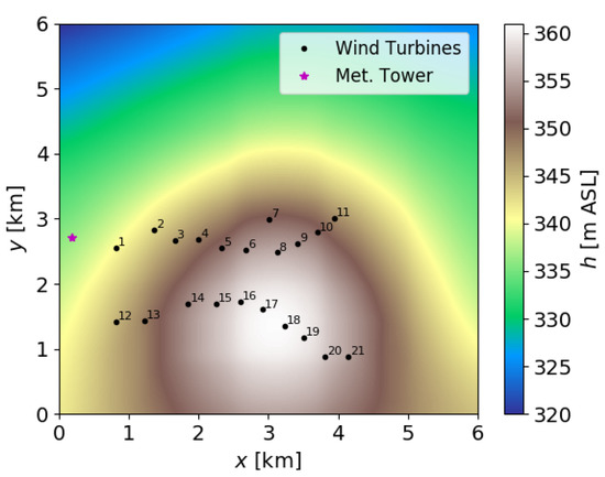
Figure 1.
Terrain height for the innermost domain, d06, shown in meters above sea level (ASL). In addition, the locations of 21 simulated wind turbines, as well as the meteorological tower used for validation in Section 2.2, are included. Note that the lidar used for validation is roughly 4 km south of the region depicted here.
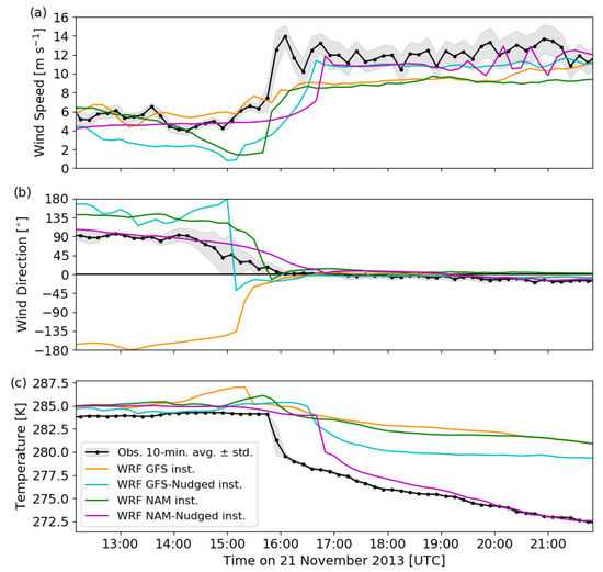
Figure 2.
Comparison of WRF modeled (a) wind speed; (b) wind direction; and (c) temperature to observations at 80 m AGL (turbine hub height). Mesoscale WRF model results (from d03) are shown as instantaneous values every 10 min for various forcing datasets and nudging options. Observations are displayed as the 10-min mean ± standard deviation, with data points at the middle of the 10-min range. In (b), the wind direction is modified for visualization purposes by subtracting 360 from values above 180 (such that 0 is northerly flow, 90 is easterly flow, −90 is westerly flow, and 180/−180 is southerly flow).
One of the benefits of using the WRF model for this multi-scale framework is the availability of atmospheric physics options. Here, the WSM 3-class microphysics scheme (), the RRTM longwave radiation scheme (), the Dudhia shortwave radiation scheme (), the Monin–Obukhov (Janjić Eta) surface layer scheme (), and the unified Noah land surface model () are used on all domains. The Kain–Fritsch cumulus parameterization () is used on the outermost domain. The reader is referred to [28] and the references therein for additional details on the WRF model’s physics schemes.
The WRF model also offers a variety of turbulence closure schemes that are appropriate for both mesoscale and LES domains. On the outer three domains (d01–d03), which can be considered mesoscale domains, planetary boundary layer (PBL) schemes are appropriate. For these domains, the Mellor–Yamada–Janjić (MYJ) scheme, which compared favorably with other closure models at a similar wind farm [41], is employed. On the inner two domains (d05 and d06), the resolution is fine enough to resolve turbulent structures, making LES more appropriate. For these domains, the TKE 1.5 order subgrid model is employed. A particular difficulty of multi-scale meteorological simulations is the parameterization of turbulence in the gray zone or terra incognita, where neither PBL nor LES closures are technically appropriate [42]. Domain d04, which has a horizontal grid spacing m, falls within the gray zone. However, in the absence of clear guidelines for turbulence parameterization at this resolution, the decision was made to nest through the gray zone using a PBL scheme on d04 to reach the region of interest on LES grids (d05 and d06).
The WRF model framework used here also includes the capability to stimulate turbulence on LES domains using a stochastic inflow perturbation method known as the cell perturbation method (CPM; [38,39]). When LES domains are initiated from a parent domain with coarser resolution, it takes time and space (fetch) to spin up turbulence on the finer domain. If turbulence takes too long to develop, this can limit the performance of the multi-scale simulation. The CPM works by applying a small temperature perturbation to the flow on the upwind domain boundaries, thus reducing turbulence spin up time and fetch for that domain. In the present simulations, the CPM is applied on the finest two domains (d05 and d06), and its effectiveness is explored below in Section 3.2 and Section 3.3.
The mesoscale portion of the model (domains d01–d03) is run from 6:00–22:00 UTC on 21 November 2013 to allow for adequate spin up before the frontal passage at roughly 16:00 UTC. The inner domains (d04–d06) are initialized from a restart file at 15:00 UTC and run until 17:00 UTC. A drawback of this setup is that the initial conditions for the inner nests must be interpolated from d03, resulting in coarse topography from d03 being used for d04–d06 (as seen in Figure 1).
Note that the topography resolution used on d03 is the standard 30 s topography data available in the WRF model package. It would, however, be computationally too expensive to run the inner domains for the full spin up period, which would be necessary to initialize them with higher-resolution topography in the standard WRF model release. Therefore, the decision was made to use the default topography so that a longer spin up time could be completed for the mesoscale domains. Future work could evaluate the nested grid setup and include higher-resolution topography, both of which are known to affect the development of turbulence on the innermost domains of multi-scale simulations.
2.2. Model Validation
To ensure that accurate mesoscale conditions are used to force flow through the wind turbine array on the innermost domain, the model is validated through comparison to nearby observations. Wind speed and temperature were measured at a nearby meteorological tower, the location of which is shown in Figure 1. Due to processing issues with the time-averaged wind direction measured on the tower, similar wind direction values are instead reported from a lidar that was positioned near the wind farm but roughly 4 km south of the region shown in Figure 1. These observations are compared to WRF model data from d03, the finest mesoscale domain, at 80 m AGL, the turbine hub height.
Comparisons for several forcing options, including NAM data with and without nudging, as well as GFS data with and without nudging, are shown in Figure 2. Note that the rotor equivalent wind speed, or average wind speed across the entire rotor disk, were also calculated; however, on this particular day, the rotor equivalent wind speed and hub-height wind speed were essentially identical. For brevity, only hub-height wind speed is shown here.
Forcing the WRF model with NAM data plus grid analysis nudging provides the best agreement with observations, capturing the overall magnitude of the wind ramp, change in wind direction, and temperature drop associated with the frontal passage. Although this is not shown, the NAM-forced WRF simulation also qualitatively captures the transition from near-neutral to slightly unstable conditions following the frontal passage, as noted by [36]. While the frontal passage happens roughly an hour late in the model with NAM plus nudging, this forcing still outperforms the other options. In what follows, all presented model results will be from this case. Additional modifications could possibly be made to better capture the time of the frontal passage, however this is not certain and is beyond the scope of the present study. Instead, model results are shifted back 50 min to allow for direct comparison between model results and radar observations during the frontal passage, which is of primary interest here.
2.3. Model Improvements
The GAD model implemented into the WRF model by [31] is used to parameterize the wind turbines’ effect on the flow within domain d06. For the present study, improvements were made to the original implementation to better simulate an operational wind farm. These include the capability of individual turbines to yaw, or rotate toward the oncoming wind [37], as well as a new turbine power calculation.
2.3.1. Turbine Yawing
Yaw error is accumulated at each time step as
where is the difference between the direction the turbine is facing and the incoming wind direction, n is the time step, and is initially 0. When the absolute value of the accumulated error exceeds a user-defined threshold, the turbine begins to yaw at a user-defined rate until , at which point is reset to 0. No yaw error is accrued while yawing is taking place. Here, an error threshold of 10,000 s (i.e., 10° of yaw error accrued for 10 s) and a yaw rate of 2° s are used.
The incoming wind direction necessary for yawing is calculated as a running average over the previous 100 time steps of the wind direction at a designated inflow point. The inflow point is chosen to be one rotor diameter upstream of the turbine hub in the direction it is currently facing, and at roughly the same height AGL as the hub (i.e., along a terrain-following grid line from the hub). The inflow velocity used in the turbine force calculations is calculated similarly at the inflow point using a running average. Turbine cut-in and cut-out capabilities have also been added such that, when the incoming wind speed for an individual turbine is outside of the cut-in/cut-out range, no turbine forces or yaw errors are calculated.
2.3.2. Turbine Power Calculation
The power output of each turbine is estimated as the power extracted from the flow by the GAD model. At each WRF model grid cell, the GAD model parameterizes the forces due to each turbines’ blades on the surrounding air, and these forces can be summed in three dimensions to calculate the power extracted by each turbine,
Here, is the rotational velocity of the turbine, r is the radial distance from each grid cell center to the turbine hub axis, is the force tangential to the rotor plane at each grid cell center, and , , and are grid cell dimensions. The factor is a Gaussian smoothing term that is a function of the normal distance from each grid cell center to the rotor plane . The reader is referred to [31,37] for additional discussion of these terms. Turbine power estimated from the WRF-GAD model is compared to observations below in Section 3.3.
3. Results
The multi-scale WRF-GAD model captures the arrival of the front, including the rotation of the wind turbines and the subsequent bending of the wakes. An animation of model results from domain d06 are included in the supplementary material (see Video S1, in Supplementary Materials). In what follows, model results will be compared to available observations of wind speed and turbine power output during the frontal passage.
3.1. Background Flow and Turbine Wake Comparison
A comparison of hub-height wind speed between the model and radar observations is shown in Figure 3. Following [36], the processed radar data can be considered a “psuedo-average” over the 80 s scanning period. However, the model results are shown as instantaneous snapshots in order to emphasize resolved turbulence structure. As previously noted, the mesoscale model forcing creates a difference in the timing of the frontal passage in the observations versus the model, and therefore the model results are shifted back 50 min to facilitate comparison with radar data.
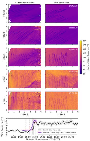
Figure 3.
Hub-height wind speed comparison between radar observations and time-shifted WRF model results at the times indicated by the dotted lines in the bottom panel. Wind speed observed at the meteorological tower at 80 m AGL, as in Figure 2, and time-shifted modeled wind speeds from domain d06 at the same height, are shown in the bottom panel, with 10-min average values shown at the middle of the 10-min range.
Even after the shift, there is a slight misalignment of the wind ramp timing at the meteorological tower (see in Figure 3, bottom panel), likely due to differences in the frontal shape and dynamics between the model and the observations. The present work is focused on comparing the modeled and observed dynamics at the wind farm, rather than focusing on the exact timing of the frontal passage as provided by the mesoscale forcing. Note also that the hub height wind speed at the tower, as shown in the bottom panel of Figure 3, is taken from the innermost domain d06, and is therefore slightly different from the hub height wind speed shown in Figure 2a, which is taken from domain d03.
Good agreement between the WRF-GAD model results and the observations is seen in the magnitude (plus or minus roughly 3 m s) and direction of the background flow, as well as in the scale and direction of the turbine wakes. The three leftmost turbines in the radar observation field are not included in the model because they were too close to the d06 boundary. Additionally, two second-row turbines that are active in the model were inactive during the observations (this is confirmed by available turbine power data) and therefore did not produce measureable wakes.
Before the frontal passage, the background flow is relatively quiescent and easterly-northeasterly. As the front passes through the array, the wind direction rotates to northerly, and the wind speed increases by nearly 10 m s. The yawing feature of the GAD model captures the resulting turbine rotation, including the bending of turbine wakes (see Figure 3, 15:38 UTC). It is important to note here that the yawing functionality of the modeled turbines is approximate because that of the real turbines is proprietary (and therefore unknown by the authors). Thus, there are likely differences in the yawing functionality between the modeled and real turbines, although this is difficult to quantify.
Following the frontal passage, increased turbulence is seen in the radar data, with large-scale “streaky” structures which are known to occur in ABL flow [43,44] oriented roughly north–south, as well as smaller-scale turbulent motions. This turbulence reduces the coherence of the turbine wakes (see discussion in [36]), making them more difficult to discern in Figure 3 (e.g., 15:47 and 16:08 UTC). The increase in turbulence intensity during the frontal passage is further evidenced by an increase in the standard deviation of the wind speed, as shown in the bottom panel of Figure 3. While both the observations and model results show an increase in the standard deviation of the wind speed as the front passes, the observed increase is larger. Increasing the intensity of resolved turbulence in the model may be addressed in future simulations by using improved turbulence downscaling techniques (see Section 3.2).
The magnitude of the turbine wakes can be quantified using the perturbation wind speed within the farm,
where W is the wind speed and is an upstream inflow wind speed (see Figure 4). Here, is estimated by averaging W along the west–east transect at km. This calculation is similar to a wake deficit but is calculated for the entire farm rather than for individual turbines. Over the time range shown in Figure 4, estimates from the radar observations vs. the model results differ by roughly 1 m s or less, providing a good baseline for comparison (see Figure 4, bottom panel).
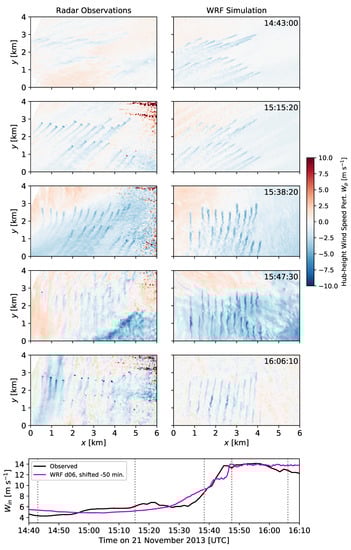
The wind speed perturbation in the turbine wakes can be as large as 10 m s, and it increases in magnitude as the background wind speed increases. Agreement in values is best prior to the frontal passage (14:43–15:38 UTC), when the background flow is more quiescent. As larger scale turbulent structures move through the turbine array during the frontal passage (15:47–16:08 UTC), the modeled results show more persistent wakes than the observations; however, the magnitude and direction of the wakes are still similar.
3.2. Turbulence Downscaling
To examine the effectiveness of the CPM in downscaling turbulence in the multi-scale WRF model, a second simulation is performed with the CPM turned off. As seen in Figure 5, which shows hub-height velocity fields, the CPM stimulates the development of smaller-scale turbulent features both before and after the frontal passage. Although the model grid is able to support these features, they do not have adequate time or fetch to develop when the CPM is not used. Thus, without the CPM, the background flow contains only weak turbulence before the frontal passage and only larger-scale turbulent structures after the frontal passage.
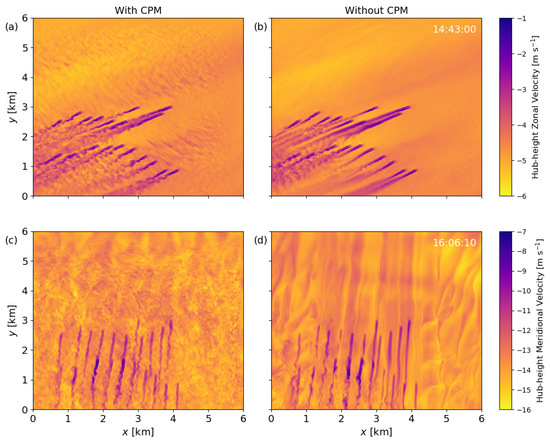
Figure 5.
Comparison of hub-height velocity between WRF model runs (a,c) with and (b,d) without the cell perturbation method. Results are shown (a,b) before the frontal passage, and (c,d) after the frontal passage. The times shown, 14:43:00 and 16:06:10 UTC (+ 50 min.), correspond to panels in Figure 3 and Figure 4.
The effect of the CPM on modeled power output is discussed in the next section. The CPM would be especially useful when examining turbulence spectra or TKE in detail; however, turbulence data are not available for comparison in this case study. In addition to using the CPM, it is also likely that improving the resolution of the topography or using a more sophisticated LES scheme would help the model capture smaller-scale turbulent structures. These ideas will be pursued in future work.
3.3. Turbine Power Output Comparison
Turbine power production is estimated from the WRF-GAD model using Equation (2) and output every minute. The 10-min averaged power predicted by the WRF model is in good agreement with the observed power. Data from select turbines (7 and 17, see locations in Figure 1) are shown in Figure 6a,b, and agreement is similar among the other modeled turbines (not shown).
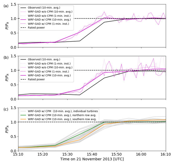
Figure 6.
Power output comparison between observations and time-shifted WRF model results, both with and without the cell perturbation method, for turbines (a) 7 and (b) 17 (see Figure 1); (c) average power output from time-shifted WRF model results with the cell perturbation method, including averages for northern and southern turbine rows.
Although the model data are shifted to improve alignment with radar data, the wind ramp still occurs roughly 10 min early in the model as opposed to the observations. This accounts for the difference in timing of the power ramp in Figure 6a,b.
High-frequency power output from the model, also shown in Figure 6a,b, reveals large power fluctuations both during and after the frontal passage event. These fluctuations are caused both by ambient turbulence and by the passage of wakes from upstream turbines, and can be greater than 0.5 MW. Turbine 7 (Figure 6a) is upstream of the other turbines and therefore experiences minimal power fluctuations, resulting only from ambient turbulence. In contrast, turbine 17 (Figure 6b) is affected by wakes from several upstream turbines (see Figure 4), and therefore experiences much larger power fluctuations, especially following the wind ramp. High frequency power data are not available for comparison.
In general, wake effects cause the average power output of the southern row of turbines to be less than that of the northern row (Figure 6c). However, after the frontal passage, the turbines in both rows are operating at or near rated power, . Similar results were found in the observed power data (compare “northern” and “southern” rows here to “northern” and “middle” rows, respectively, in [36], Figure 7). By modifying the resolved turbulence in the model, the CPM also has an effect on the turbine power output. The effect is larger during and after the frontal passage as the flow becomes more turbulent. While the effect of the CPM on the upstream turbine is minimal (Figure 6a), the CPM helps to reduce the overestimate in power after the frontal passage for the downstream turbine (Figure 6b).
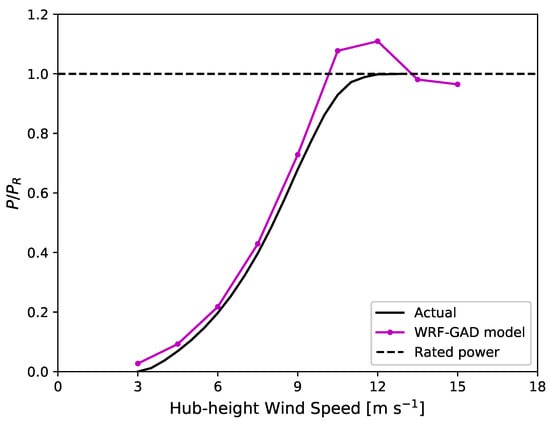
Figure 7.
Comparison of WRF-GAD model power curve, created using idealized simulations with flat terrain and a constant forcing velocity, to actual power curve for the turbines in the study area.
A power curve was constructed for the WRF-GAD model using idealized simulations with flat terrain and a constant forcing velocity (see Figure 7).
While the WRF-GAD model power curve generally follows the actual power curve, it tends to overestimate power when wind speeds are in the range of 10–13 m s. This helps to explain the general overestimate of power by the WRF-GAD model following the wind ramp event (after roughly 15:45 UTC in Figure 6), when the ambient wind speed is roughly within this range. The overestimated power is likely a result of the simplifications inherent to the GAD model parameterization, and could be improved in future studies.
4. Conclusions
A multi-scale WRF model framework has been used to simulate wind farm performance during a frontal passage event. To the knowledge of the authors, this is the first seamless multi-scale simulation of such a case. Using grid nesting, the model transitions from mesoscale to large-eddy simulation with an embedded wind turbine parameterization, the generalized actuator disk model implemented into the WRF model by [31]. Several updates were made to this parameterization to simulate realistic turbine operations, including a yawing capability and a power output calculation. Furthermore, the cell perturbation method was used to improve the downscaling of turbulent structures within the region of interest.
When compared to novel radar observations, the model was shown to capture both the dynamics of the frontal passage and the turbine response, after accounting for a time shift in the mesoscale forcing data. Model predictions showed remarkably good agreement with observed turbine wake structure, velocity perturbation, and power output. The updated yawing feature of the GAD model captured the resulting turbine rotation accurately, including the bending of turbine wakes. In general, wake effects caused the average power output of the southern row of turbines to be less than that of the northern row, and turbines in both rows were at or near rated power following the frontal passage, as seen in the observed power data. These results demonstrate the promise of the WRF-GAD model framework for multi-scale simulations of wind farm operation.
Future studies could utilize this framework, in combination with new observations, to examine other important interactions between wind farms and complex atmospheric dynamics. Of particular interest is the comparison of modeled and observed turbulence quantities, which were not available in this study. Of additional interest are atmospheric stability effects, such as the presence of cold pools and low level jets, which are known to modulate wind farm power output and cause issues balancing the electrical grid [45]. Since many wind farms are located in regions of complex terrain such as mountains, valleys, and ridges, it is also critical to accurately predict turbine response to terrain-induced flows [46]. By combining the benefits of a numerical weather prediction model with those of a microscale wind turbine simulation, the WRF-GAD model framework is well suited to take on these modeling challenges.
Supplementary Materials
The following is available online at https://doi.org/10.5281/zenodo.3579571, Video S1: Multi-scale simulation of flow through a wind farm during a frontal passage event.
Author Contributions
Writing—original draft preparation and visualization, R.S.A. and N.M.; writing—review and editing, J.D.M., B.D.H., J.L.S., S.W., and F.K.C.; methodology, software, validation, and formal analysis, R.S.A., J.D.M., and N.M.; conceptualization, N.M., J.D.M., and F.K.C.; investigation and data curation, B.D.H., J.L.S., and S.W. All authors have read and agreed to the published version of the manuscript.
Funding
This work was prepared by LLNL under Contract DE-AC52-07NA27344. R.S.A., J.D.M., and S.W. were supported by the U.S. DOE Wind Energy Technologies Office. N.M. was supported by the Lawrence Scholar program at LLNL.
Acknowledgments
We acknowledge three anonymous reviewers for their suggestions to improve the manuscript. Note that a portion of this work is included in the PhD thesis of N.M. at the University of California, Berkeley, entitled “Simulation of the atmospheric boundary layer for wind energy applications” (2015). This work was also presented by F.K.C. at the 2019 North American Wind Energy Academy (NAWEA)/WindTech conference in Amherst, MA. However, this work has not been published previously in a peer-reviewed journal.
Conflicts of Interest
The authors declare no conflict of interest. The funders had no role in the design of the study; in the collection, analyses, or interpretation of data; in the writing of the manuscript, or in the decision to publish the results.
Abbreviations
The following abbreviations are used in this manuscript:
| ABL | Atmospheric boundary layer |
| AGL | Above ground level |
| ASL | Above sea level |
| CFD | Computational fluid dynamics |
| CPM | Cell perturbation method |
| GAD | Generalized actuator disk |
| GFS | Global forecast system |
| LES | Large-eddy simulation |
| MYJ | Mellor–Yamada–Janjić |
| NAM | North American Mesoscale |
| NCEP | National Centers for Environmental Prediction |
| PBL | Planetary boundary layer |
| TKE | Turbulence kinetic energy |
| UTC | Coordinated universal time |
| WRF | Weather Research and Forecasting |
References
- Högström, U.; Asimakopoulos, D.N.; Kambezidis, H.; Helmis, C.G.; Smedman, A. A field study of the wake behind a 2 MW wind turbine. Atmos. Environ. 1988, 22, 803–820. [Google Scholar] [CrossRef]
- Barthelmie, R.J.; Pryor, S.C.; Frandsen, S.T.; Hansen, K.S.; Schepers, J.G.; Rados, K.; Schlez, W.; Neubert, A.; Jensen, L.E.; Neckelmann, S. Quantifying the impact of wind turbine wakes on power output at offshore wind farms. J. Atmos. Ocean. Tech. 2010, 27, 1302–1317. [Google Scholar] [CrossRef]
- Magnusson, M.; Smedman, A.S. Air flow behind wind turbines. J. Wind. Eng. Ind. Aerod. 1999, 80, 169–189. [Google Scholar] [CrossRef]
- Thomsen, K.; Sørensen, P. Fatigue loads for wind turbines operating in wakes. J. Wind. Eng. Ind. Aerod. 1999, 80, 121–136. [Google Scholar] [CrossRef]
- Kelley, N.D.; Jonkman, B.J.; Scott, G.N.; Bialasiewicz, J.T.; Redmond, L.S. Impact of Coherent Turbulence on Wind Turbine Aeroelastic Response and Its Simulation: Preprint; Technical Report; National Renewable Energy Laboratory: Golden, CO, USA, 2005. [Google Scholar]
- Churchfield, M.J.; Lee, S.; Michalakes, J.; Moriarty, P.J. A numerical study of the effects of atmospheric and wake turbulence on wind turbine dynamics. J. Turbul. 2012, 13, N14. [Google Scholar] [CrossRef]
- Elliott, D.L.; Barnard, J.C. Observations of wind turbine wakes and surface roughness effects on wind flow variability. Sol. Energy 1990, 45, 265–283. [Google Scholar] [CrossRef]
- Ammara, I.; Leclerc, C.; Masson, C. A viscous three-dimensional differential/actuator-disk method for the aerodynamic analysis of wind farms. J. Sol. Energ.-T. ASME 2002, 124, 345–356. [Google Scholar] [CrossRef]
- Lundquist, J.K.; DuVivier, K.K.; Kaffine, D.; Tomaszewski, J.M. Costs and consequences of wind turbine wake effects arising from uncoordinated wind energy development. Nature Energy 2019, 4, 26–34. [Google Scholar] [CrossRef]
- Pryor, S.C.; Shepherd, T.J.; Volker, P.J.H.; Hahmann, A.N.; Barthelmie, R.J. “Wind Theft” from Onshore Wind Turbine Arrays: Sensitivity to Wind Farm Parameterization and Resolution. J. Appl. Meteorol. Clim. 2020, 59, 153–174. [Google Scholar] [CrossRef]
- Stevens, R.J.A.M.; Meneveau, C. Flow structure and turbulence in wind farms. Annu. Rev. Fluid Mech. 2017, 49, 311–339. [Google Scholar] [CrossRef]
- Calaf, M.; Meneveau, C.; Meyers, J. Large eddy simulation study of fully developed wind-turbine array boundary layers. Phys. Fluids 2010, 22, 015110. [Google Scholar] [CrossRef]
- Meyers, J.; Meneveau, C. Optimal turbine spacing in fully developed wind farm boundary layers. Wind Energy 2012, 15, 305–317. [Google Scholar] [CrossRef]
- Meyers, J.; Meneveau, C. Large eddy simulations of large wind-turbine arrays in the atmospheric boundary layer. In Proceedings of the 48th AIAA Aerospace Sciences Meeting, Orlando, FL, USA, 4–7 January 2010; p. 827. [Google Scholar]
- Calaf, M.; Parlange, M.B.; Meneveau, C. Large eddy simulation study of scalar transport in fully developed wind-turbine array boundary layers. Phys. Fluids 2011, 23, 126603. [Google Scholar] [CrossRef]
- Porté-Agel, F.; Wu, Y.T.; Lu, H.; Conzemius, R.J. Large-eddy simulation of atmospheric boundary layer flow through wind turbines and wind farms. J. Wind. Eng. Ind. Aerod. 2011, 99, 154–168. [Google Scholar] [CrossRef]
- Porté-Agel, F.; Wu, Y.T.; Chen, C.H. A numerical study of the effects of wind direction on turbine wakes and power losses in a large wind farm. Energies 2013, 6, 5297–5313. [Google Scholar] [CrossRef]
- Wu, Y.T.; Porté-Agel, F. Modeling turbine wakes and power losses within a wind farm using LES: An application to the Horns Rev offshore wind farm. Renew. Energy 2015, 75, 945–955. [Google Scholar] [CrossRef]
- Creech, A.; Früh, W.G.; Maguire, A.E. Simulations of an offshore wind farm using large-eddy simulation and a torque-controlled actuator disc model. Surv. Geophys. 2015, 36, 427–481. [Google Scholar] [CrossRef]
- Nilsson, K.; Ivanell, S.; Hansen, K.S.; Mikkelsen, R.; Sørensen, J.N.; Breton, S.P.; Henningson, D. Large-eddy simulations of the Lillgrund wind farm. Wind Energy 2015, 18, 449–467. [Google Scholar] [CrossRef]
- Eriksson, O.; Lindvall, J.; Breton, S.P.; Ivanell, S. Wake downstream of the Lillgrund wind farm: A Comparison between LES using the actuator disc method and a Wind farm Parametrization in WRF. J. Phys. Conf. Ser. 2015, 625, 012028. [Google Scholar] [CrossRef]
- Abkar, M.; Sharifi, A.; Porté-Agel, F. Wake flow in a wind farm during a diurnal cycle. J. Turbul. 2016, 17, 420–441. [Google Scholar] [CrossRef]
- Guggeri, A.; Draper, M. Large-eddy Simulation of an Onshore Wind Farm with the Actuator Line Model Including Wind Turbine’s Control below and above Rated Wind Speed. Energies 2019, 12, 3508. [Google Scholar] [CrossRef]
- Zajaczkowski, F.J.; Haupt, S.E.; Schmehl, K.J. A preliminary study of assimilating numerical weather prediction data into computational fluid dynamics models for wind prediction. J. Wind. Eng. Ind. Aerod. 2011, 99, 320–329. [Google Scholar] [CrossRef]
- Churchfield, M.J.; Michalakes, J.; Vanderwende, B.; Lee, S.; Sprague, M.A.; Lundquist, J.K.; Moriarty, P.J. Using Mesoscale Weather Model Output as Boundary Conditions for Atmospheric Large-Eddy Simulations and Wind-Plant Aerodynamic Simulations; Technical Report; National Renewable Energy Laboratory: Golden, CO, USA, 2013. [Google Scholar]
- Gopalan, H.; Gundling, C.; Brown, K.; Roget, B.; Sitaraman, J.; Mirocha, J.D.; Miller, W.O. A coupled mesoscale–microscale framework for wind resource estimation and farm aerodynamics. J. Wind. Eng. Ind. Aerod. 2014, 132, 13–26. [Google Scholar] [CrossRef]
- Santoni, C.; García-Cartagena, E.J.; Ciri, U.; Zhan, L.; Valerio Iungo, G.; Leonardi, S. One-way mesoscale-microscale coupling for simulating a wind farm in North Texas: Assessment against SCADA and LiDAR data. Wind Energy 2020, 1–20. [Google Scholar] [CrossRef]
- Skamarock, W.C.; Klemp, J.B.; Dudhia, J.; Gill, D.O.; Barker, D.M.; Duda, M.G.; Huang, X.; Wang, W.; Powers, J.G. A Description of the Advanced Research WRF Version 3; NCAR Technical note NCAR/TN-475+STR; National Center for Atmospheric Research: Boulder, CO, USA, 2008. [Google Scholar]
- Fitch, A.C.; Olson, J.B.; Lundquist, J.K.; Dudhia, J.; Gupta, A.K.; Michalakes, J.; Barstad, I. Local and mesoscale impacts of wind farms as parameterized in a mesoscale NWP model. Mon. Wea. Rev. 2012, 140, 3017–3038. [Google Scholar] [CrossRef]
- Volker, P.H.J.; Badger, J.; Hahmann, A.N.; Ott, S. The Explicit Wake Parametrisation V1.0: A wind farm parametrisation in the mesoscale model WRF. Geosci. Model Dev. 2015, 8, 3715–3731. [Google Scholar] [CrossRef]
- Mirocha, J.D.; Kosovic, B.; Aitken, M.L.; Lundquist, J.K. Implementation of a generalized actuator disk wind turbine model into the Weather Research and Forecasting model for large-eddy simulation applications. J. Renew. Sustain. Energy 2014, 6, 013104. [Google Scholar] [CrossRef]
- Aitken, M.L.; Kosović, B.; Mirocha, J.D.; Lundquist, J.K. Large eddy simulation of wind turbine wake dynamics in the stable boundary layer using the Weather Research and Forecasting Model. J. Renew. Sustain. Energy 2014, 6, 033137. [Google Scholar] [CrossRef]
- Mirocha, J.D.; Rajewski, D.A.; Marjanovic, N.; Lundquist, J.K.; Kosović, B.; Draxl, C.; Churchfield, M.J. Investigating wind turbine impacts on near-wake flow using profiling lidar data and large-eddy simulations with an actuator disk model. J. Renew. Sustain. Energy 2015, 7, 043143. [Google Scholar] [CrossRef]
- Vanderwende, B.J.; Kosović, B.; Lundquist, J.K.; Mirocha, J.D. Simulating effects of a wind-turbine array using LES and RANS. J. Adv. Model. Earth Syst. 2016, 8, 1376–1390. [Google Scholar] [CrossRef]
- Marjanovic, N.; Mirocha, J.D.; Kosović, B.; Lundquist, J.K.; Chow, F.K. Implementation of a generalized actuator line model for wind turbine parameterization in the Weather Research and Forecasting model. J. Renew. Sustain. Energy 2017, 9, 063308. [Google Scholar] [CrossRef]
- Hirth, B.D.; Schroeder, J.L.; Irons, Z.; Walter, K. Dual-Doppler measurements of a wind ramp event at an Oklahoma wind plant. Wind Energy 2015, 19, 953–962. [Google Scholar] [CrossRef]
- Marjanovic, N. Simulation of the Atmospheric Boundary Layer for Wind Energy Applications. Ph.D. Thesis, University of California, Berkeley, CA, USA, 2015. [Google Scholar]
- Muñoz-Esparza, D.; Kosović, B.; Mirocha, J.D.; van Beeck, J. Bridging the transition from mesoscale to microscale turbulence in numerical weather prediction models. Bound.-Layer Meteor. 2014, 153, 409–440. [Google Scholar] [CrossRef]
- Muñoz-Esparza, D.; Kosović, B.; Van Beeck, J.; Mirocha, J.D. A stochastic perturbation method to generate inflow turbulence in large-eddy simulation models: Application to neutrally stratified atmospheric boundary layers. Phys. Fluids 2015, 27, 035102. [Google Scholar] [CrossRef]
- Wharton, S.; Newman, J.F.; Qualley, G.; Miller, W.O. Measuring turbine inflow with vertically-profiling lidar in complex terrain. J. Wind Eng. Ind. Aerod. 2015, 142, 217–231. [Google Scholar] [CrossRef]
- Marjanovic, N.; Wharton, S.; Chow, F.K. Investigation of model parameters for high-resolution wind energy forecasting: Case studies over simple and complex terrain. J. Wind Eng. Ind. Aerod. 2014, 134, 10–24. [Google Scholar] [CrossRef]
- Wyngaard, J.C. Toward numerical modeling in the Terra Incognita. J. Atmos. Sci. 2004, 61, 1816–1826. [Google Scholar] [CrossRef]
- Hutchins, N.; Marusic, I. Evidence of very long meandering features in the logarithmic region of turbulent boundary layers. J. Fluid Mech. 2007, 579, 1–28. [Google Scholar] [CrossRef]
- Ludwig, F.L.; Chow, F.K.; Street, R.L. Effect of turbulence models and spatial resolution on resolved velocity structure and momentum fluxes in large-eddy simulations of neutral boundary layer flow. J. Appl. Meteor. Climatol. 2009, 48, 1161–1180. [Google Scholar] [CrossRef]
- Shaw, W.J.; Berg, L.K.; Cline, J.; Draxl, C.; Djalalova, I.; Grimit, E.P.; Lundquist, J.K.; Marquis, M.; McCaa, J.; Olson, J.B.; et al. The Second Wind Forecast Improvement Project (WFIP2): General Overview. Bull. Am. Meteorol. Soc. 2019, 100, 1687–1699. [Google Scholar] [CrossRef]
- Fernando, H.J.S.; Mann, J.; Palma, J.M.L.M.; Lundquist, J.K.; Barthelmie, R.J.; Belo-Pereira, M.; Brown, W.O.J.; Chow, F.K.; Gerz, T.; Hocut, C.M.; et al. The Perdigao: Peering into microscale details of mountain winds. Bull. Am. Meteorol. Soc. 2019, 100, 799–819. [Google Scholar] [CrossRef]


© 2020 by the authors. Licensee MDPI, Basel, Switzerland. This article is an open access article distributed under the terms and conditions of the Creative Commons Attribution (CC BY) license (http://creativecommons.org/licenses/by/4.0/).