Article

Application of Data Fusion Techniques to Improve Air Quality Forecast: A Case Study in the Northern Italy

Department of Mechanical and Industrial Engineering (DIMI), University of Brescia, via Branze 38, 25123 Brescia, Italy
*
Author to whom correspondence should be addressed.
Atmosphere 2020, 11(3), 244; https://doi.org/10.3390/atmos11030244
Submission received: 8 January 2020 / Revised: 12 February 2020 / Accepted: 25 February 2020 / Published: 29 February 2020
(This article belongs to the Special Issue Air Quality Control and Planning)

Abstract

:
Deterministic air quality forecasting models play a key role for regional and local authorities, being key tools to ensure that timely information about actual or near future exceedances of pollutant threshold values are provided to the public, as stated by the EU directive (2008/50/EC). One of the main problems of these models is that they usually underestimate some important pollutants, like PM10, especially in high-concentration areas. For this reason, the forecast of critical episodes (i.e., exceedance of 50 μ g/m 3 for PM10 concentration daily threshold) has low accuracy. To overcome this issue, several computationally fast techniques have been implemented in the last decade. In this work, two computational fast techniques are introduced, implemented and evaluated. The techniques are based on the off-line correction of the chemical transport model output in the forecasting window, estimated by means of the measurement data up to the beginning of the forecast. In particular, the techniques are based on the estimation of the correction performed as a linear combination of the corrections computed for the days when the measurements are available. The resulting system has been applied to the Lombardy region case (Northern Italy) for daily PM10 forecasting with good results.

1. Introduction

According to the 2018 Lancet Commission on Pollution and Health report [1], air pollution caused 16% of the deaths due to non-natural causes (around 9 million people) worldwide in 2015. In particular, particulate matter (PM) exposure strongly affects human health, because high PM levels are linked to premature mortality, through pulmonary and cardio-vascular diseases [2,3]. In order to limit the population health risks, the European Commission in the Directive (2008/50/EC) recommends the member states to promptly give the population the information about expected PM exceedances. In the last decades, a number of decision-support systems has been developed [4] in order to help regional and local authorities to reach this objective. Even if in literature there is plenty of support systems developed to define long term plans for the pollutant exposure reduction [5,6,7,8], the formalization and implementation of decision support systems to develop short term plan is still in its infancy. The core of these systems formalization and development is the air quality forecasting model, needed to accurately reproduce the dynamics of the phenomena related to the formation, accumulation and removal of pollutants in the atmosphere. Air quality forecasting systems can be classified in (1) data-driven models and (2) deterministic chemical and transport models [9].
Data-driven air quality models are more related to system identification theory than air quality physics. In particular, they are implemented defining a general family of mathematical relationships among causes and effects calibrated from tuples of input and output data. The causes, for example, can be the level of emissions of a set of pollutant precursors inside and outside the investigated domain, meteorology data in a certain area, concentrations of a group of pollutants in previous temporal steps; the considered effects are usually the forecasted concentration of a pollutant (or many pollutants). The main advantage of these models is that they require limited computing resources and are easier to be implemented [10]. In [11] the use of multiple linear regression models combining information of the present-day about PM10 concentration and meteorological forecasts of wind speed and precipitation rate is presented. They evaluate the daily PM10 concentrations forecasting during a winter period in three cities in the western Alpe–Adria region. Data-driven air quality models include feedforward neural networks (FFNNs): they have been used to predict ozone and PM10 over the urban area of Milan, comparing the prediction performances to other two approaches derived from machine learning, pruned neural networks and lazy learning [12]. FFNNs were also used in a Northern Italy domain, in combination with a co-kriging technique allowing to improve the spatial interpolation where no dense data are available [13]. In [14] data-driven air quality models based on FFNNs are used to forecast hourly PM10 concentrations at 4 measurement locations in Athens using meteorological inputs and PM10 concentrations in previous temporal steps.
On the other hand, chemical and transport models (CTMs) are extremely complex systems considering explicitly the chemical and physical aspects of the problem. CTMs require many inputs: meteorology, temporally and chemically speciated emissions, land cover and boundary conditions and they are computationally very expensive [15]. A number of models have been set up for the forecasting application: MM5-CMAQ-EMIMO (OPANA V4) modeling system has been implemented in experimental mode to produce daily European Air Quality Forecasts for Europe with 50 km spatial resolution [16]; the PREV’AIR system provides real-time information about air pollutant concentrations, as well as long term trends, throughout Europe using the CTMs CHIMERE and MOCAGE. The PREV’AIR project introduced also the assimilation of ground in-situ observation data in the system [17]. LOTOS-EUROS has been applied by [18] to forecast PM10 concentration in the Netherlands with a 25 km resolution, performances were evaluated considering observation data and forecast provided by PROPART, the Dutch operational statistical model. More recently, MACC-I/MACC-II/MACC-III projects (Monitoring Atmospheric Composition and Climate) were developed. The air quality system integrates and analyses seven state-of-art regional CTMs and provides 96 hours forecasts of the main pollutants over the European continent [19]. For many decades data assimilation has been used to improve weather forecast in dynamic meteorology [20], since the late 1990s data assimilation was used also in air quality to generate air pollutants concentrations maps, define boundary conditions and model parameters. CTMs do not require the integration with measurements, but since the 2000s, integration techniques have been applied to atmospheric chemistry too, in order to reach better performances [21]. [22] compared the performances of two data assimilation techniques (optimal interpolation and Kalman filtering) to assess exceedances of the daily and annual mean limit values for PM10 computed with the already mentioned LOTOS-EUROS model.
CTMs data assimilation techniques can be classified in:
  • Off-line re-analysis techniques, performing an ex-post integration of the measurements with the model results, once they are computed. Off-line techniques usually include statistical methodologies: optimal interpolation methods [23], kriging and cokriging techniques [24,25]. These techniques allow, for example, the computing of reanalyzed spatial concentration fields or, in the forecasting applications, the best known estimate of the initial condition for the next day/hour [26]. In [27] a bias correction technique is presented showing a good increase in the forecasting performances for PM, ozone and nitrogen oxides.
  • On-line data assimilation techniques fully integrate the impact of the measurements directly inside the model during the simulation. They can include variational methods (2D-, 3D, 4D-var) aimed at minimizing the distance between estimated concentration and observed data ([28]) or ensemble methodologies mainly applied for ozone or nitrogen dioxide concentrations [29,30]. The main drawback of these approaches is that their implementation usually needs strong changes in the core model code [21].
This work is focused on the use of an optimal interpolation-based data fusion technique to perform the re-analysis of the Comprehensive Air Quality Model with eXtensions (CAMx), [31], results for the forecast of PM10 daily average concentrations. The presented technique is relatively simple to implement and does not require changes to be made in the CTM code. The methodology is applied in the Lombardy region, Italy.

2. Materials and Methods

Figure 1 presents the implemented methodology components and their relationship. At time t, the system computes the forecasting of PM10 concentration P M 10 R ^ ( t + 1 , . . . , t + n ) at time t + 1 , . . . , t + n using the results of a re-analysis phase that integrates the output of the CAMx model ( P M 10 G ( t ) ) and the measurements ( P M 10 ( t ) ¯ ) available at the beginning of the forecast. The methodology has three main scopes:
  • setup of the best initial condition ( P M 10 R ( t ) ) for the forecast;
  • estimation of the correction ( Δ ^ ) for the forecasting steps t + 1 , . . . , t + n ;
  • application of estimated correction Δ ^ to the forecast computed by CAMx model P M 10 G ( t + 1 , . . . , t + n ) .
In the next subsections, the main components of the system will be presented: the Chemical Transport Model, CAMx, the re-analysis technique and the two different correction estimation Δ ^ methodologies, namely a weighted mean approach and a least-square error approach.

2.1. CAMx Model

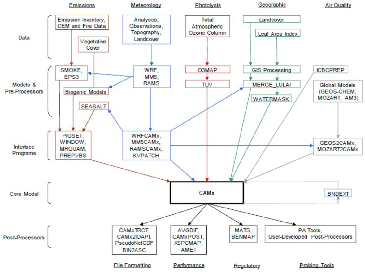
The Comprehensive Air quality Model with extensions [31] is an open-source state-of-the-science multi-scale photochemical model for gas and particulate air pollution based on Fortran source code. CAMx simulates the emission, dispersion, chemical reaction and removal of pollutants by solving the Eulerian continuity equations forward in time for each chemical species [32,33]. CAMx needs detailed input related to:
  • gridded and point source emission data;
  • meteorology defined through the use of prognostic meteorological models (for example WRF [34]);
  • photolysis rates for the photochemical mechanism;
  • land cover information;
  • boundary conditions are available from global models.
Figure 2 [31] presents all the modules, processors and interface between the CAMx and the different information sources used to produce its input.

2.1.1. Re-analysis Phase

The re-analysis phase has been implemented following an Optimal Interpolation approach [35]. This state-of-the-art method allows the merging of available observations with the simulation results of a model, taking into account the relayability of both the model and the measurements [36]. More information about the theoretical background related to the optimal interpolation can be found in [35], while information about the application of this method to air quality can be found in [37]. As stated at the beginning of Section 2, once the last available measurement has been used to re-analyze the model output in order to obtain the best possible initial condition for the forecasting phase, the re-analyzed field is used to compute the correction bias to be applied to the forecasted fields. In the following, let P M 10 G ( t ) be the PM10 concentration computed through the CTM model at time t and P M 10 R ( t ) = P M 10 G ( t ) + Δ ( t ) the estimated PM10 concentration after the correction Δ ( t ) due to the optimal interpolation technique. Moreover, let Δ ^ ( t + 1 , . . . , t + n ) be the estimated value of the correction Δ at time t + 1 , . . . , t + n to be used during the forecasting horizon.

2.1.2. Optimal Interpolation

The Optimal Interpolation technique is a Best Linear Unbiased Estimator (BLUE) estimator of the true state of a system. In particular, the re-analyzed field P M 10 R ( t ) describing the PM10 concentrations over a certain grid at time t can be computed as:
P M 10 R ( t ) = P M 10 ( t ) + K ( t ) · ( P M 10 ¯ ( t ) - H · P M 10 G ( t ) ) ,
where:
  • P M 10 R ( t ) is the re-analyzed PM10 fields at time t;
  • P M 10 G ( t ) is the background field at time t, i.e., the output of CAMx model before integration with the measurements;
  • P M 10 ¯ ( t ) are the (pointwise) measurements of PM10 at monitoring station locations;
  • H is a mathematical operator allowing to extract the background concentrations at the monitoring locations.
  • K ( t ) is a matrix gain, often called Kalman gain, computed in order to minimize the variance of the errors.
It can be proved ([35]) that:
K = P · H T ( · H · P · H T + R ) - 1 ,
where P and R are the covariance matrix of the background and measurement errors, respectively. One of the main points affecting the value of K is the definition of the values of P and R. Matrix P is usually estimated following a Gaussian approach as:
P = [ p i , j ] = e x p ( - d ( i , j ) 2 2 · L h 2 ) · v = D ( i , j ) · v ,
where D = d ( i , j ) is a matrix defining the decreasing of the variance with respect to the distance between the center of the cells i and j, L h is a parameter defining the decay of covariance with respect to the distance, and v is the model error variance estimate, computed on the basis of previous simulation results.
Usually, R is a diagonal matrix, as the instruments errors are independent. Moreover, if the used instruments are similar, all the monitoring stations can be considered having the same error variance of r, leading to R = r I , where I is the identity matrix.
With this assumption, Equation (2) can be written as:
K = D H T · v ( v · ( H D H T + r v · I ) ) - 1 = D H T ( H D H T + σ · I ) - 1 ,
where σ = r / v can be seen as a measure of the goodness of the measurements with respect to the model and it is the only degree of freedom to be selected.
Once that the value of K and subsequently P M 10 R ( t ) have been found, the value of Δ ( t ) at time t can be expressed as:
Δ ( t ) = P M 10 R ( t ) - P M 10 G ( t ) .
It can be noticed that (1) mathematically, Δ ( t ) has the same dimension of P M 10 G ( t ) (and P M 10 R ( t ) ), equal to the number of grid cells; (2) since it is an a posteriori technique, this procedure clearly works only if the measurement P M 10 ¯ ( t ) are known. For these reasons some adaptations/additions have to be performed in order to solve the forecasting problem.

2.1.3. Weighted Mean Approach

In this approach, the correction for the next n times is computed as the weighted mean of the two last available corrections Δ ( t ) and Δ ( t - 1 ) (Equation (6)):
Δ ^ ( t + n ) = α Δ ( t ) + ( 1 - α ) Δ ( t - 1 ) .
This very simple approach is based on the assumption that the value of the error on the results of the CTM at time t is strongly related to the errors at previous times. It can be easily noticed that for α = 1 , the value of the estimated correction at time t + n is equal to the correction at time t (persistent model) and for α = 0 . 5 the estimation is the arithmetic mean of the two last corrections. The crucial aspects of this approach are related to the choice of the parameter α .

2.1.4. Least-square Error Approach

In this approach, the correction is computed applying the least-square error technique to the last available corrections:
Δ ^ ( t + n ) = α 0 + i = 1 m α i Δ ( t - i ) ,
where α i , i = 0 , . . . , m are computed applying the least-square errore technique to the correction at time t (dependent variable) and the m previous corrections at time t - i (independent variables). The value m is called order (or memory) of the model.
More in details, let t ¯ be the last day the system is able to perform the re-analysis using the measurements (i.e., the last day when the measurements are available). The estimation of the parameter vector α of a m order model for the computation of Δ ( t ¯ + n ) is performed through the following steps:
  • Collecting all the Δ ( t ) , t = t ¯ - m - n . . . , t ¯ ;
  • Defining the output matrix Y L S including the values of Δ for each cell of the domain at time t ¯ (last Δ available);
  • Defining the input matrix I L S including for the first m columns the value of Δ for each cell of the domain at time t = t ¯ - m - n . . . t ¯ - 1 - n , and as a last column a vector of value equal to 1, in order to compute the depolarization term ( α 0 ).
  • Applying the least square Equation ((8)) for linear parameter models:
    α = ( I L S T · I L S ) - 1 · I L S · Y L S .

3. Case Study

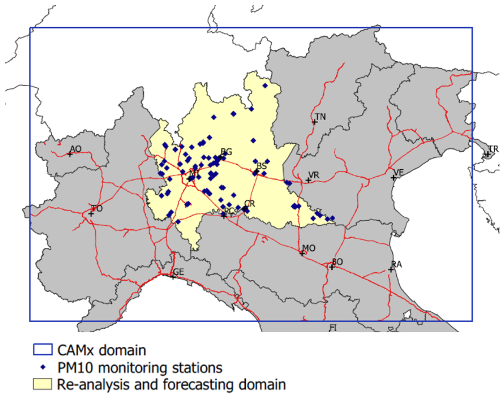
The methodology has been evaluated for the daily PM10 forecast on a Lombardy region (Northern Italy) domain (Figure 3), an area often characterized by high PM10 concentration levels leading to critical episodes (daily mean concentration higher than 50 μ g/m 3 ). In particular, the system has been run for the entire 2011 year and the forecast up to 3 days in advance has been computed. The selected domain covers a 540 × 360 km 2 area with a 6 × 6 km 2 spatial resolution. Emission input is provided by the INEMAR and EMEP [38] emission inventories. Table 1 presents total annual emission for each macro-sector for the year on the domain under study. The data include VOC, CO, NOx, NH3, SO2, PM10 and PM2.5 annual emissions for each cell of the domain. Monthly, daily and hourly pollutant specific temporal profiles are applied for different emission sources, seasons of the year and types of days (weekdays, days before holiday and holidays). Chemical characterization of VOC and physicochemical characterization of PM is performed using chemical and granulometric speciation profiles dependent on the emission activity. Meteorological input has been computed starting from the results of the WRF model. The 70 PM10 stations of the Lombardy region monitoring network were used for the integration of the CAMx results with the measurements. Fourteen tests have been performed grouped as:
  • a test (CAMx) with only measurement data used to correct the initial condition of the forecast;
  • 11 tests computed applying the methods in Section 2.1.3 with α ranging from 0 to 1 with a step of 0.1;
  • two tests with integration performed following the least-square error approach (Section 2.1.4) with m = 2 ( L S 2 ) and m = 3 ( L S 3 ).
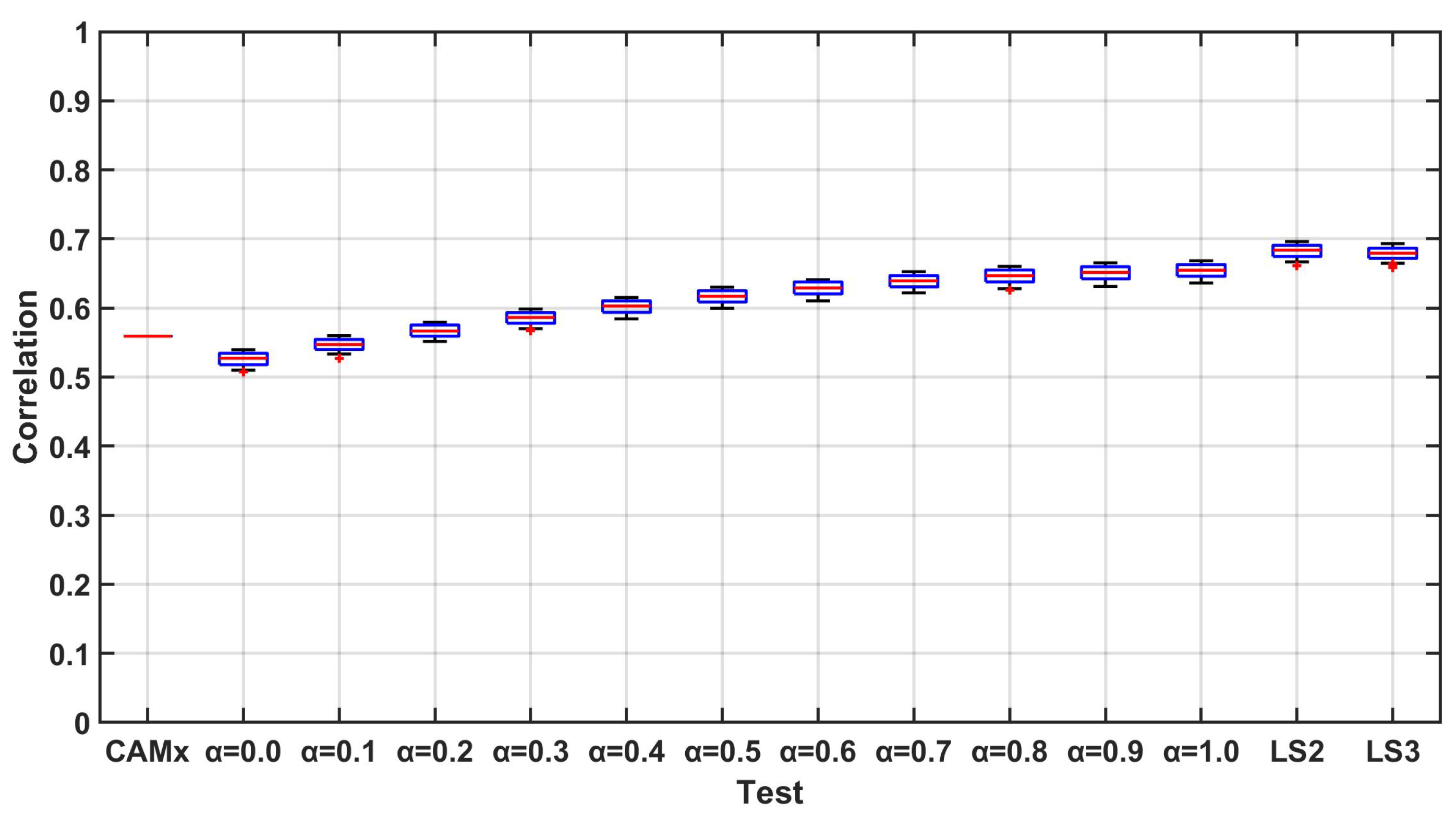
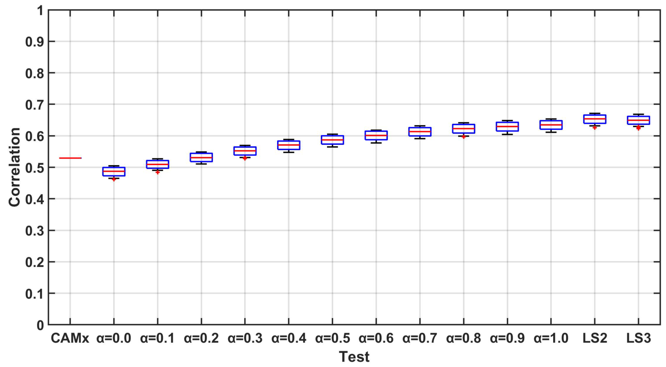
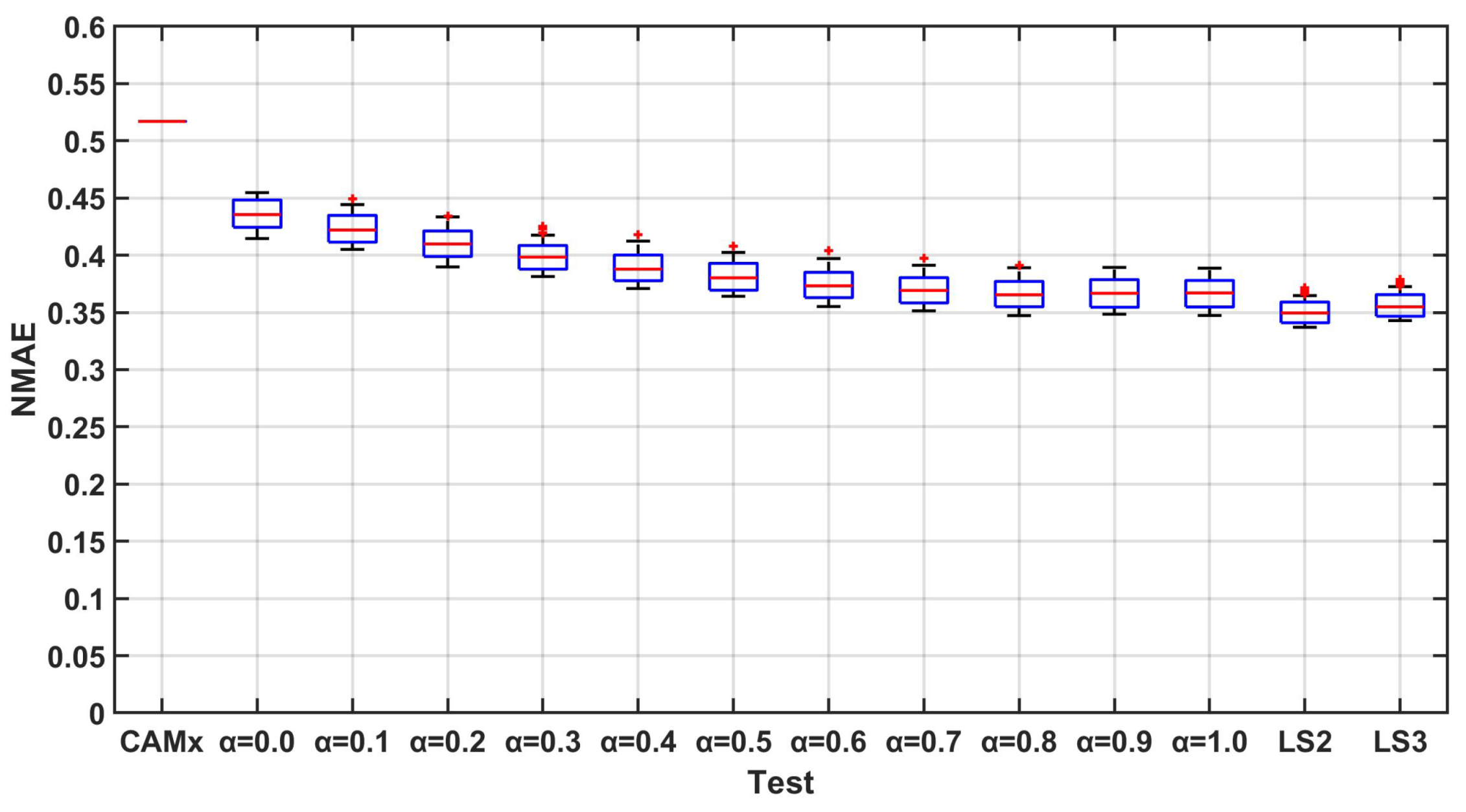
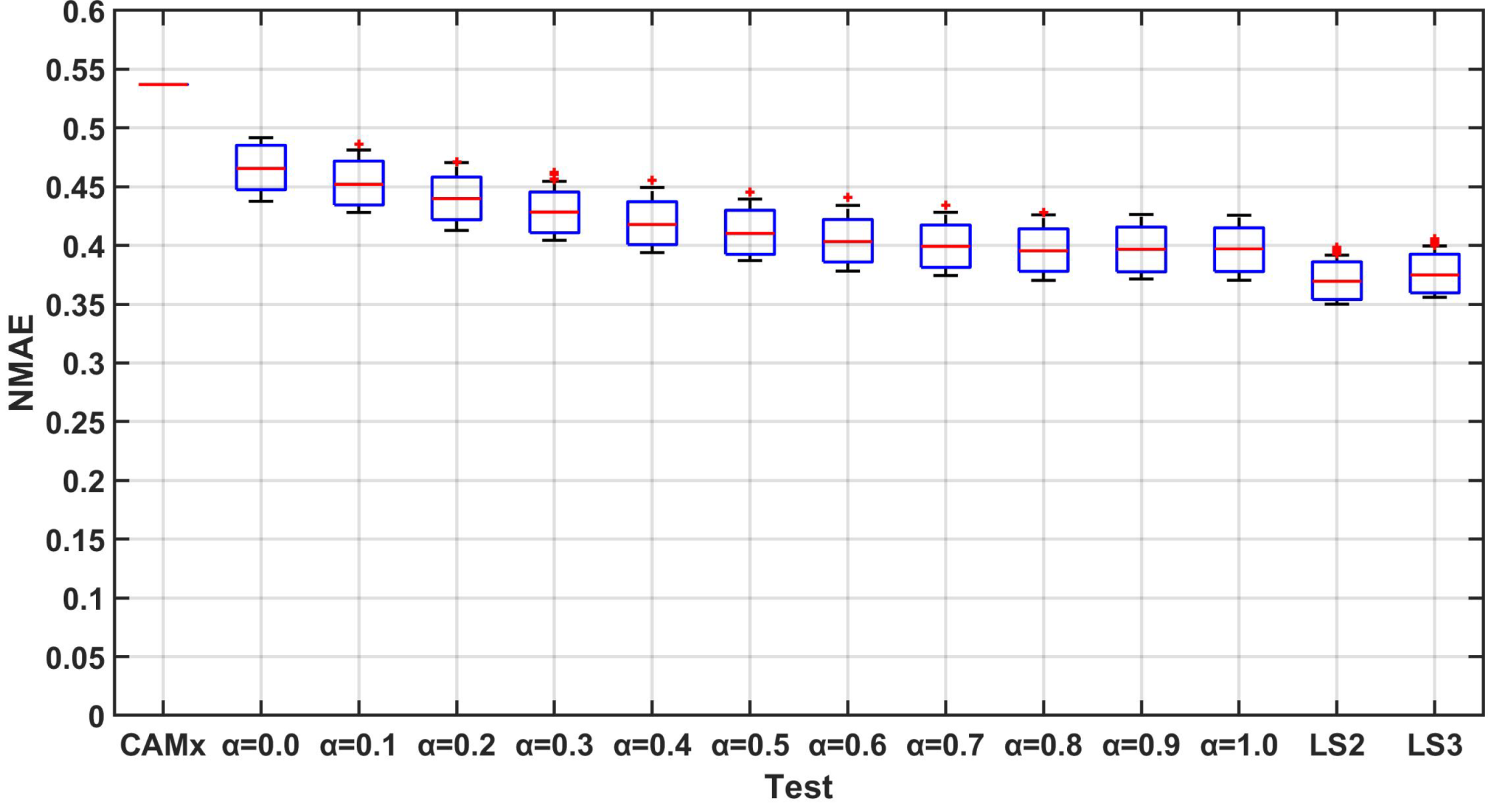
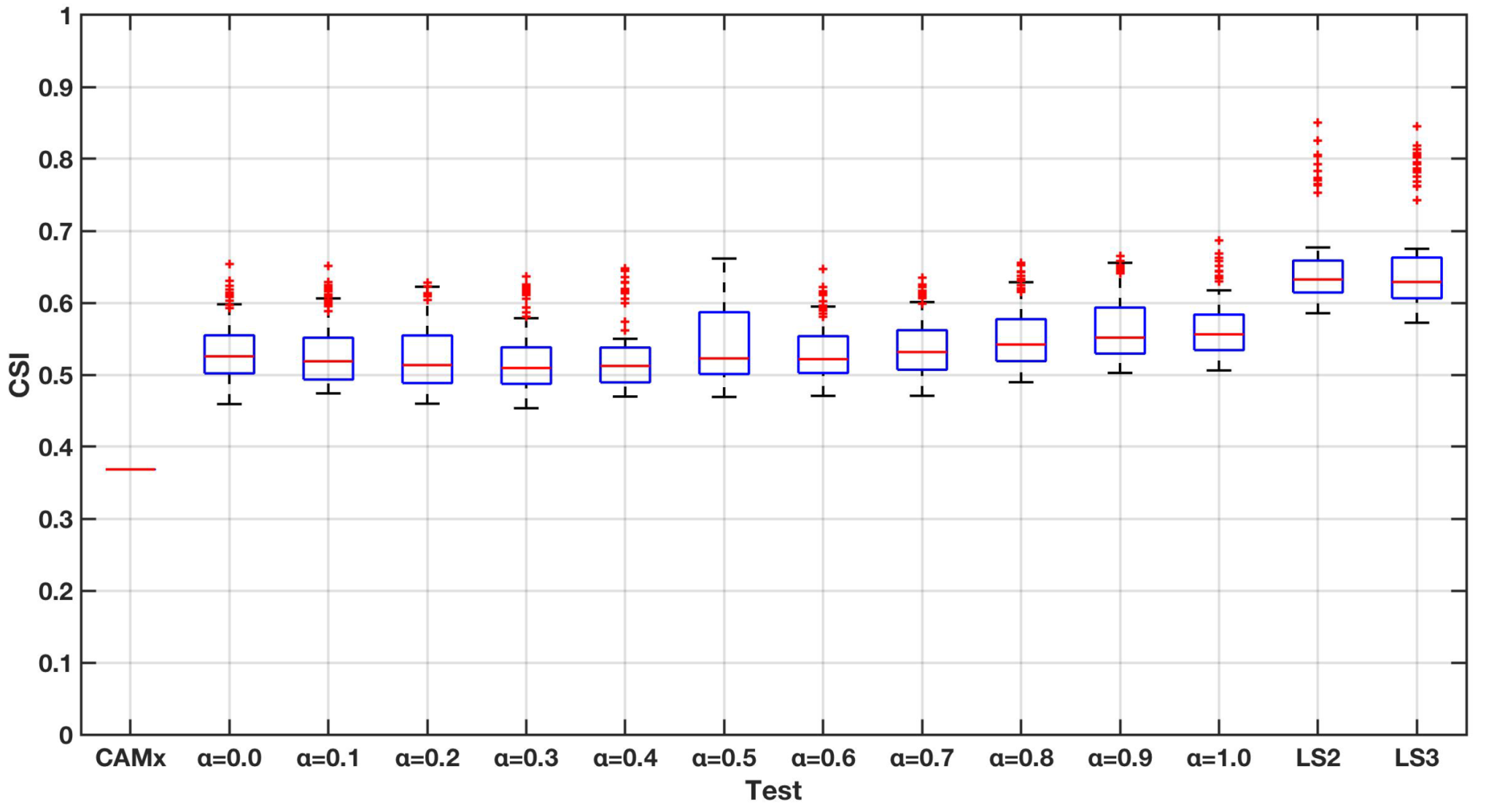
Following the idea presented in [36], in order to correctly evaluate the performance and uncertainty of the methodology, a Monte Carlo approach has been followed. In particular, 100 tests have been performed, randomly selecting 20% of the stations for the validation phase and using the remaining 80% for the optimal interpolation. The performances have been evaluated comparing the daily PM10 measured by the monitoring stations with the results of the system. The validation has been performed in two phases. In the first one, the forecasts have been evaluated using two different statistical indexes, namely the correlation coefficient and the normalized mean absolute error (NMAE). During the second phase, the capability of the model to correctly reproduce the critical events, expressed in terms of concentrations higher than the 50 μ g / m 3 threshold, has been evaluated. Figure 4, Figure 5 and Figure 6 present the boxplot of correlation coefficient for the different performed tests. It can be easily seen that for the one-step-ahead forecast, the integration techniques ensures better results with respect to the “standard” case ( C A M x ). In general, the values of the coefficient is higher for the L S test, but the use of a memory m = 3 did not grant an increase in performances. Moreover, the values of the index computed for the least square approach are comparable to those of the best weighted mean approach model, obtained for α = 1 (persistent model). All the cases show a limited variability of the performances for the different tests, as highlighted by the boxes tops (1st and 3rd quartile) close to the median. Increasing the forecasting horizon to 2 and 3 steps causes a general worsening of the performances, in particular for lower value of α . In fact for α < 0 . 3 the worsening is so high that the C A M x case shows better or comparable performances. The least-square error approach shows lower sensitivity to the forecasting horizon, presenting a median that in these cases are consistently higher than the one of all the other tests (Figure 5 and Figure 6). The performances in terms of normalized mean absolute error (NMAE, Figure 7, Figure 8 and Figure 9) shows a bigger impact of the presented integration procedures. In this case, the value of the index computed for α and L S tests is always better than that granted by C A M x even when the forecasting horizon increases. This can be explained by the fact that almost all the techniques are able to compensate for the underestimation of the PM10 concentrations typical of the models. The second part of the validation is more related to the objective of the forecasting system. It is a matter of fact that Local Authorities need a forecasting system able to reproduce the critical situation. For what concerns PM10, the critical situations are related to the exceedances of the concentration of 50 μ g/m 3 as a daily mean. In order to evaluate the capability of the model to correctly reproduce these events, the Critical Success Index (CSI) also known as Threat Score has been computed for all the performed tests. The CSI can be computed starting from the contingecy table in Table 2 as:
C S I = Y Y / ( Y Y + N Y + Y N ) .
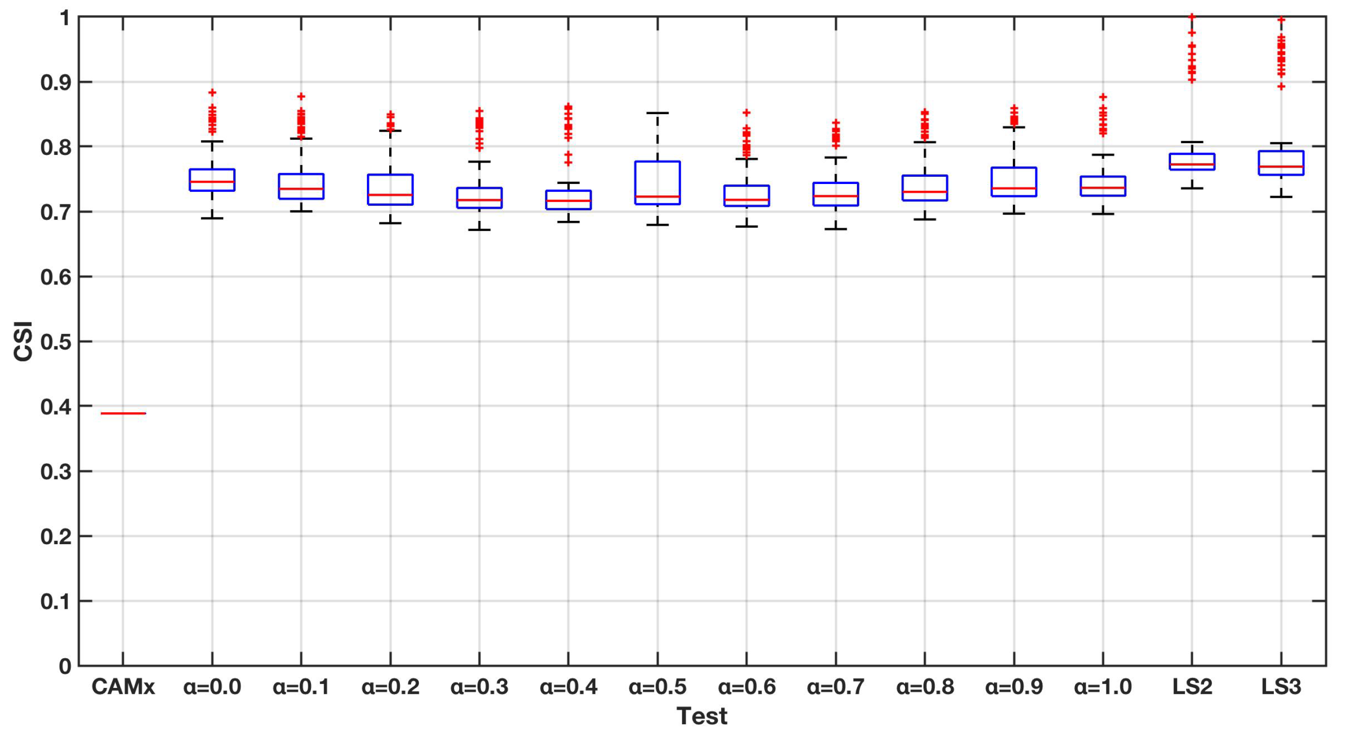
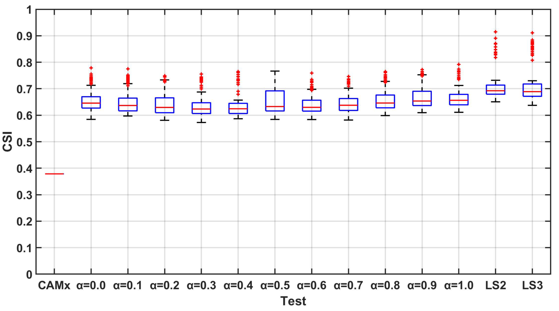
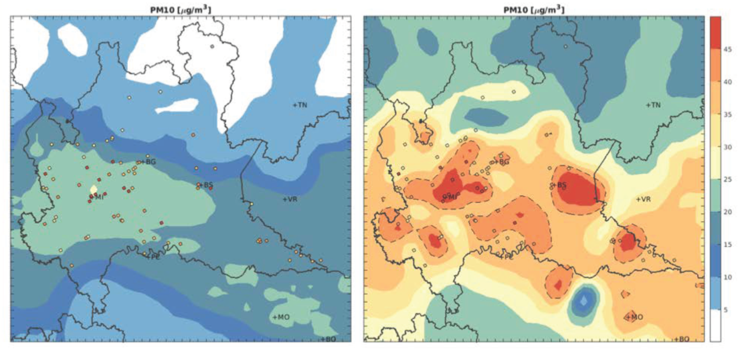
The values of the index range from 0 (worst case) to 1 (perfect case). In particular, this index expresses the capability of the system to correctly reproduce the critical events and include a penalty due to the false alarms. Figure 10, Figure 11 and Figure 12 presents the results for this index. The increasing in the performances with respect to the case without assimilation is very high for all the performed tests. Still, the L S techniques ensure better performances with respect to all the other tests. Increasing the forecasting horizon, the performances get worse quickly for all the tests and a slight increase in the distance of the values between weighted mean case and L S case can be seen even if no differences in the performances can be noticed between the L S 2 and L S 3 cases, suggesting that an increase in the memory of the system would not ensure better results. Finally, an example of the technical performance is reported in Figure 13, where the CAMx and LS3 t+1 yearly mean PM10 concentrations forecast are shown and compared to the values measured by the regional monitoring networks. The impact of the performances is clearly visible.

4. Conclusions

The paper presents two techniques allowing integration between model results and measurement data for forecasting applications. The techniques are based on the estimation of the correction to be added to CTM results in the forecasting horizon on the basis of the results of the optimal interpolation computed between measurements and models up to the beginning of the forecast. Two different approaches have been tested: (i) a simple, weighted mean approach based on the last two computed corrections and (ii) a more complex least-square error approach based on the estimation of the linear regression coefficient linking the last correction occurrences. In both of these cases, the computation is fast and does not need any change in the CTM model code. The methodology has been integrated on a CAMx based system for the computation of PM10 concentration and the overall system has been applied to a domain placed in Northern Italy and including the whole Lombardy region. The selection of the model and the domain is driven by the need to use a state-of-the-art system in a really challenging domain. As a matter of fact, Eulearian chemical transport models heavily underestimate PM10 concentrations in this area, making them difficult to use for the forecast of the PM10 critical levels and in particular of the exceedances days. The integration of the two techniques led to significantly increased skill of the forecast with the correlation coefficient exceeding 0.75 and success index close to 0.8. Those indexes showed a significant improvement in all the tests with respect to the chemical transport model forecast. The sensitivity analysis of the forecast skill with respect to the forecasting horizon has been performed indicating the performance of the integrated system deteriorating slightly faster with respect to the chemical transport model most likely due to not considering meteorological data forecast. Nevertheless, the performances of the integrated systems always remain higher than the chemical transport model one. The uncertainty in the results has been assessed using a Montecarlo approach. The assessment shows the robustness of the methodology with respect to the selection of the available measurement station locations. For these reasons and in the light of the obtained performances, the presented integration methodology seems to lead to an overall system that can be used by the Local Authorities to perform the forecasting of critical events of PM10. The methodology is applicable to other primary and secondary pollutants like ozone and nitrogen oxides at different scales and in different domains, even if some peculiarity of the considered pollutants have to be considered, in particular, the impact of very localised emissions of nitrogen oxides. Our future efforts will focus on detailed evaluation of the impact of the number of stations used and the sensitivity analysis of the parameter sigma value in Equation (4).

Author Contributions

Conceptualization, C.C. and E.T.; Data curation, C.C. and E.D.A.; Funding acquisition, C.C., G.F. and M.V.; Methodology, C.C., E.D.A., E.T. and M.V.; Project administration, C.C. and G.F.; Resources, M.V.; Software, C.C.; Supervision, M.V.; Validation, E.D.A. and E.T.; Writing—original draft, C.C., E.D.A., G.F. and E.T. All authors have read and agreed to the published version of the manuscript.

Funding

This research received no external funding.

Conflicts of Interest

The authors declare no conflict of interest.

Abbreviations

The following abbreviations and notations are used in this manuscript:
CAMxComprehensive Air quality Model with extension
CMAQCommunity Multiscale Air Quality model
COCarbon monoxide
CORINAIRCore inventory air emissions
CTMChemical Transport Model
DSSDecision Support System
EMEPEuropean Monitoring and Evaluation Programme
EMIMOEmission Model
FFNsFeedforward Neural Networks
LOTOS-EUROSLong Term Ozone Simulation-European Operational Smog
MACCMonitoring Atmospheric Composition and Climate
MM5Fifth-Generation Mesoscale Model
NH3Ammonia
NOxNitrogen oxides
PMParticulate Matter
PM10Particulate Matter with diameter lower than 10 μ m
PREV’AIRPrevisions et Observations de la Qualite de l’Air en France et en Europe
PROPARTDutch PM forecast statistical model
SO2Sulphur dioxide
WRFWeather Research and Forecasting model
P M 10 R ^ ( t ) PM10 Estimated re-analyzed field forecasted at time t (output of the system)
P M 10 R ( t ) PM10 computed re-analyzed field at time t (computed on the basis of measurement)
P M 10 ¯ ( t ) PM10 measurements vector at time t
P M 10 G ( t ) PM10 background field at time t (output of CAMx model)
VOCVolatile Organic Compounds
Δ ( t ) Correction computed on the basis of the available measurement at time t
Δ ^ ( t ) Correction estimated at time t

References

  1. Landrigan, P.J.; Fuller, R.; Acosta, N.J.R.; Adeyi, O.; Arnold, R.; Basu, N.N.; Baldé, A.B.; Bertollini, R.; Bose-O’Reilly, S.; Boufford, J.I.; et al. The Lancet Commission on pollution and health. Lancet 2018, 391, 462–512. [Google Scholar] [CrossRef] [Green Version]
  2. Pope, C.; Dockery, D. Acute health effects of PM10 pollution on symptomatic and non-symptomatic children. Am. Rev. Respir. Dis. 1992, 145, 1123–1128. [Google Scholar] [CrossRef]
  3. Pope, C.; Dockery, D.; Spengler, J.; Raizenne, M. Respiratory health and PM10 pollution. A daily time series analysis. Am. Rev. Respir. Dis. 1991, 144, 668–674. [Google Scholar] [CrossRef]
  4. Blond, N.; Carnevale, C.; Douros, J.; Finzi, G.; Guariso, G.; Janssen, S.; Maffeis, G.; Martilli, A.; Pisoni, E.; Real, E.; et al. A framework for integrated assessment modelling. In SpringerBriefs in Applied Sciences and Technology; Springer: Berlin, Germany, 2017; pp. 9–35. [Google Scholar]
  5. Turrini, E.; Carnevale, C.; Finzi, G.; Volta, M. A non-linear optimization programming model for air quality planning including co-benefits for GHG emissions. Sci. Total Environ. 2018, 621, 980–989. [Google Scholar] [CrossRef]
  6. Relvas, H.; Miranda, A.; Carnevale, C.; Maffeis, G.; Turrini, E.; Volta, M. Optimal air quality policies and health: A multi-objective nonlinear approach. Environ. Sci. Pollut. Res. 2017, 24, 13687–13699. [Google Scholar] [CrossRef]
  7. Carnevale, C.; Finzi, G.; Pederzoli, A.; Turrini, E.; Volta, M.; Ferrari, F.; Gianfreda, R.; Maffeis, G. Impact of pollutant emission reductions on summertime aerosol feedbacks: A case study over the PO valley. Atmos. Environ. 2015, 122, 41–57. [Google Scholar] [CrossRef]
  8. Turrini, E.; Vlachokostas, C.; Volta, M. Combining a Multi-Objective Approach and Multi-Criteria Decision Analysis to Include the Socio-Economic Dimension in an Air Quality Management Problem. Atmosphere 2019, 10, 381. [Google Scholar] [CrossRef] [Green Version]
  9. Seinfeld, J.H.; Pandis, S.N. Atmospheric Chemistry and Physics; John Wiley & Sons: Hoboken, NJ, USA, 1997. [Google Scholar]
  10. Carnevale, C.; Finzi, G.; Pisoni, E.; Volta, M. Lazy Learning based surrogate models for air quality planning. Environ. Model. Softw. 2016, 83, 47–57. [Google Scholar] [CrossRef]
  11. Stadlober, E.; Hörmann, S.; Pfeiler, B. Quality and performance of a PM10 daily forecasting model. Atmos. Environ. 2008, 42, 1098–1109. [Google Scholar] [CrossRef]
  12. Corani, G. Air quality prediction in Milan: Feed-forward neural networks, pruned neural networks and lazy learning. Ecol. Model. 2005, 185, 513–529. [Google Scholar] [CrossRef] [Green Version]
  13. Carnevale, C.; Finzi, G.; Pisoni, E.; Singh, V.; Volta, M. An integrated air quality forecast system for a metropolitan area. J. Environ. Monit. 2011, 13, 3437–3447. [Google Scholar] [CrossRef]
  14. Grivas, G.; Chaloulakou, A. Artificial neural network models for prediction of PM10 hourly concentrations, in the Greater Area of Athens, Greece. Atmos. Environ. 2006, 40, 1216–1229. [Google Scholar] [CrossRef]
  15. Carnevale, C.; Finzi, G.; Pederzoli, A.; Pisoni, E.; Thunis, P.; Turrini, E.; Volta, M. Applying the delta tool to support the Air Quality Directive: Evaluation of the TCAM chemical transport model. Air Qual. Atmos. Health 2014, 7, 335–346. [Google Scholar] [CrossRef]
  16. José, R.S.; Pérez, J.L.; Morant, J.L.; González, R.M. European operational air quality forecasting system by using MM5–CMAQ–EMIMO tool. Simul. Model. Pract. Theory 2008, 16, 1534–1540. [Google Scholar] [CrossRef]
  17. Honoré, C.; Menut, L.; Bessagnet, B.; Meleux, F.; Rouïl, L.; Vautard, R.; Poisson, N.; Peuch, V. PREV’AIR: A Platform for Air Quality Monitoring and Forecasting; Development in Environmental Science, Elsevier: Amsterdam, The Netherlands, 2007; Volume 6, pp. 292–300. [Google Scholar]
  18. Manders, A.; Schaap, M.; Hoogerbrugge, R. Testing the capability of the chemistry transport model LOTOS-EUROS to forecast PM10 levels in the Netherlands. Atmos. Environ. 2009, 43, 4050–4059. [Google Scholar] [CrossRef]
  19. Marécal, V.; Peuch, V.H.; Andersson, C.; Andersson, S.; Arteta, J.; Beekmann, M.; Benedictow, A.; Bergström, R.; Bessagnet, B.; Cansado, A.; et al. A regional air quality forecasting system over Europe: The MACC-II daily ensemble production. Geosci. Model. Dev. 2015, 8, 2777–2813. [Google Scholar] [CrossRef] [Green Version]
  20. Ghil, M.; Malanotte-Rizzoli, P. Data Assimilation in Meteorology and Oceanography. Adv. Geophys. 1991, 33, 141–266. [Google Scholar]
  21. Bocquet, M.; Elbern, H.; Eskes, H.; Hirtl, M.; Žabkar, R.; Carmichael, G.R.; Flemming, J.; Inness, A.; Pagowski, M.; Camaño, J.L.P.; et al. Data assimilation in atmospheric chemistry models: Current status and future prospects for coupled chemistry meteorology models. Atmos. Chem. Phys. 2015, 15, 5325–5358. [Google Scholar] [CrossRef] [Green Version]
  22. Denby, B.; Schaap, M.; Segers, A.; Builtjes, P.; Horálek, J. Comparison of two data assimilation methods for assessing PM10 exceedances on the European scale. Atmos. Environ. 2008, 42, 7122–7134. [Google Scholar] [CrossRef]
  23. Blond, N.; Bel, L.; Vautard, R. Three-dimensional ozone data analysis with an air quality model over the Paris area. J. Geophys. Res. Atmos. 2003, 108, 4744. [Google Scholar] [CrossRef]
  24. Van de Kassteele, J.; Koelemeijer, R.; Dekkers, A.; Schaap, M.; Homan, C.; Stein, A. Statistical mapping of PM10 concentrations over Western Europe using secondary information from dispersion modeling and MODIS satellite observations. Stoch. Environ. Res. Risk Assess. 2006, 21, 183–194. [Google Scholar] [CrossRef]
  25. Horálek, J.; Denby, B.; de Smet, P.; de Leeuw, F.; Kurfürst, P.; Swart, R.; van Noije, T. Spatial Mapping of Air Quality for European Scale Assessment; ETC/ACC: Copenhagen, Denmark, 2006. [Google Scholar]
  26. Curier, R.; Timmermans, R.; Calabretta-Jongen, S.; Eskes, H.; Segers, A.; Swart, D.; Schaap, M. Improving ozone forecasts over Europe by synergistic use of the LOTOS-EUROS chemical transport model and in-situ measurements. Atmos. Environ. 2012, 60, 217–226. [Google Scholar] [CrossRef]
  27. Neal, L.; Agnew, P.; Moseley, S.; Ordonez, C.; Savage, N.; Tilbee, M. Application of a statistical post-processing technique to a gridded, operational, air quality forecast. Atmos. Environ. 2014, 98, 385–393. [Google Scholar] [CrossRef]
  28. Eibern, H.; Schmidt, H. A four-dimensional variational chemistry data assimilation scheme for Eulerian chemistry transport modeling. J. Geophys. Res. Atmos. 1999, 104, 18583–18598. [Google Scholar] [CrossRef]
  29. Van Loon, M.; Builtjes, P.J.; Segers, A. Data assimilation of ozone in the atmospheric transport chemistry model LOTOS. Environ. Model. Softw. 2000, 15, 603–609. [Google Scholar] [CrossRef]
  30. Constantinescu, E.M.; Sandu, A.; Chai, T.; Carmichael, G.R. Assessment of ensemble-based chemical data assimilation in an idealized setting. Atmos. Environ. 2007, 41, 18–36. [Google Scholar] [CrossRef]
  31. Environ. CAMx User’s Guide Version 6.50. Available online: http://www.camx.com/files/camxusersguide_v6-50.pdf (accessed on 8 January 2020).
  32. Carnevale, C.; De Angelis, E.; Finzi, G.; Pederzoli, A.; Turrini, E.; Volta, M. A non linear model approach to define priority for air quality control. IFAC-PapersOnLine 2018, 51, 210–215. [Google Scholar] [CrossRef]
  33. Carnevale, C.; De Angelis, E.; Finzi, G.; Turrini, E.; Volta, M. An integrated forecasting system for air quality control. In Proceedings of the 2019 18th European Control Conference, ECC 2019, Budapest, Hungary, 23–26 August 2019; pp. 830–835. [Google Scholar]
  34. Skamarock, W.; Klemp, J.; Dudhia, J.; Gill, D.; Barker, D.; Duda, M.; Huang, X.; Wang, W.; Powers, J. A Description of the Advanced Research WRF Version 3: NCAR/TN-475; National Center for Atmospheric Research: Boulder, CO, USA, 2008; Volume 88. [Google Scholar]
  35. Evensen, G. Inverse methods and data assimilation in nonlinear ocean models. Phys. D Nonlinear Phenom. 1994, 77, 108–129. [Google Scholar] [CrossRef]
  36. Carnevale, C.; Finzi, G.; Pederzoli, A.; Pisoni, E.; Thunis, P.; Turrini, E.; Volta, M. A methodology for the evaluation of re-analyzed PM 10 concentration fields: A case study over the PO Valley. Air Qual. Atmos. Health 2015, 8, 533–544. [Google Scholar] [CrossRef]
  37. Candiani, G.; Carnevale, C.; Finzi, G.; Pisoni, E.; Volta, M. A comparison of reanalysis techniques: Applying optimal interpolation and Ensemble Kalman Filtering to improve air quality monitoring at mesoscale. Sci. Total Environ. 2013, 458–460, 7–14. [Google Scholar] [CrossRef]
  38. Vestreng, V.; Adams, M.; Goodwin, J. Inventory Review 2004. Emission Data Reportedd to CRLTAP and under the NEC Directive; EMEP/EEA: Copenhagen, Denmark, 2004. [Google Scholar]
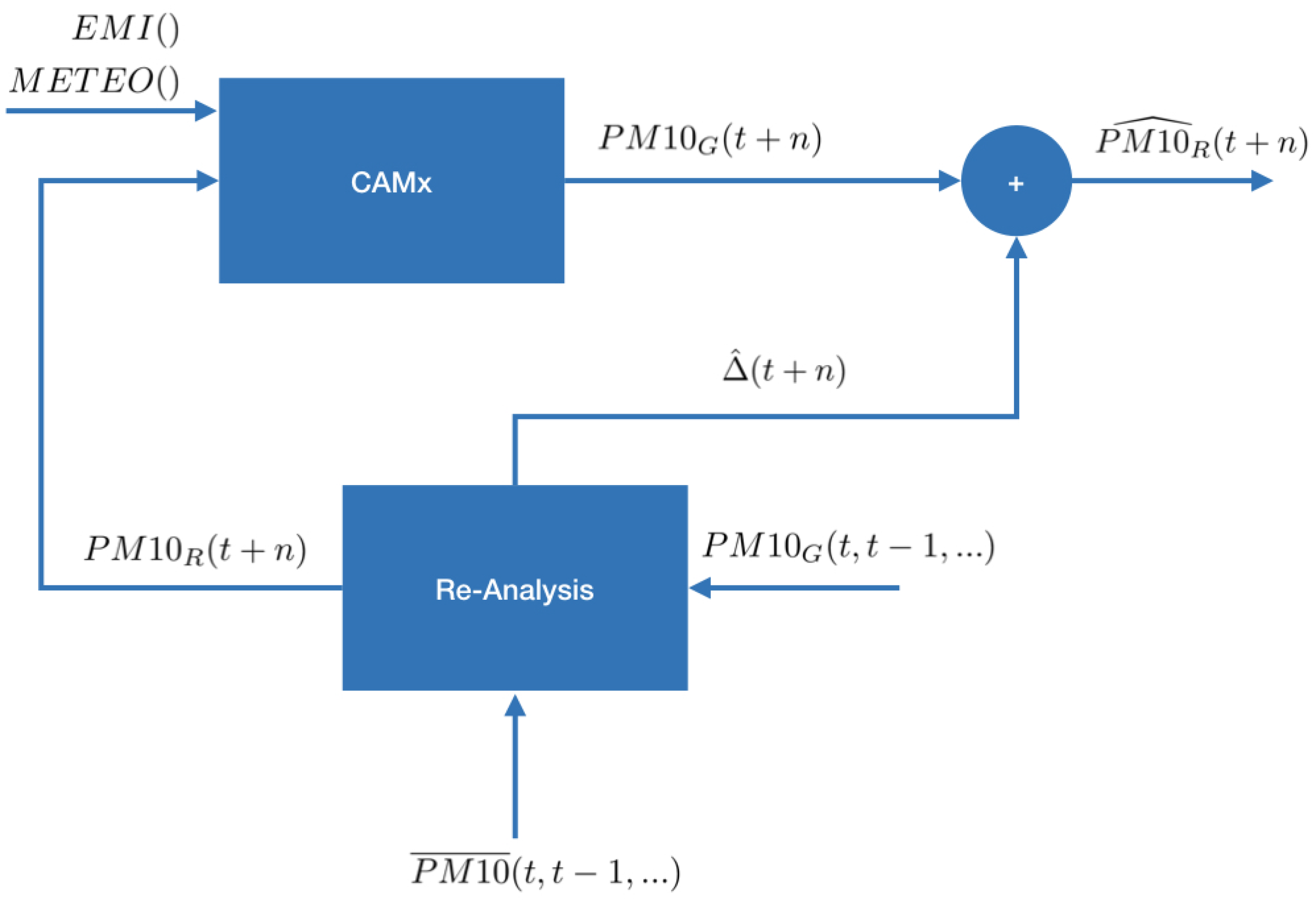
Figure 1. Diagram of the implemented system.
Atmosphere 11 00244 g001
Figure 2. Schematic diagram of the Comprehensive Air Quality Model with eXtensions (CAMx) modelling system.
Atmosphere 11 00244 g002
Figure 3. CAMx computational domain (blue rectangle) with PM10 measuring station of the Lombardy region monitoring network (blue dots) and re-analysis and forecasting techniques computing domain (yellow).
Atmosphere 11 00244 g003
Figure 4. Correlation for the one-step-forward forecast.
Atmosphere 11 00244 g004
Figure 5. Correlation for the two-step-forward forecast.
Atmosphere 11 00244 g005
Figure 6. Correlation for the three-step-forward forecast.
Atmosphere 11 00244 g006
Figure 7. NMAE for the one-step-forward forecast.
Atmosphere 11 00244 g007
Figure 8. NMAE for the two-step-forward forecast.
Atmosphere 11 00244 g008
Figure 9. NMAE for the three-step-forward forecast.
Atmosphere 11 00244 g009
Figure 10. SI for the one-step-forward forecast.
Atmosphere 11 00244 g010
Figure 11. SI for the two-step-forward forecast.
Atmosphere 11 00244 g011
Figure 12. SI for the three-step-forward forecast.
Atmosphere 11 00244 g012
Figure 13. PM10 daily average concentration maps ( μ g/m 3 ) for CAMx and LS3 t + 1 forecasting. The dots represents the PM10 concentration values measured by the monitoring network.
Atmosphere 11 00244 g013
Table 1. Total annual emission [t/yr] over the CAMx domain for each pollutant and core inventory air emissions (CORINAIR) macrosectors for the year 2011.
CORINAIR MacrosectorVOCNH3NOxPM10PM2.5SO2
Combustion in energy and transformation industries30155933,5959428269641
Non-industrial combustion plants73,197109046,26744,06443,248622
Combustion in manufacturing industry823377872,0224934343529730
Production processes40,056121212,9504425240816,440
Fossil fuel and geothermal energy distribution28,187035882741257
Solvent and other product use232,831103680107285313
Road transport68,7064831260,82921,93016,479644
Other mobile sources and machinery15,3291565,095629750044446
Waste treatment and disposal337627086348115310571185
Agriculture153,400304,835651375212957222
Biogenic205,6064212,79810,1426173234
TOTAL831,936315,673517,455102,56282,51464,434
Table 2. Contingecy table.
ForecastedObservedTotal
YesNo
YesHits (YY)False Alarm (YN)YY+YN
NoMissess (NY)Correctly Rejected (NN)NY+NN
TotalYY+NYYN+NNYY+YN+NY+NN