Evaluation of a New Statistical Method—TIN-Copula–for the Bias Correction of Climate Models’ Extreme Parameters


Abstract
1. Introduction
2. Data
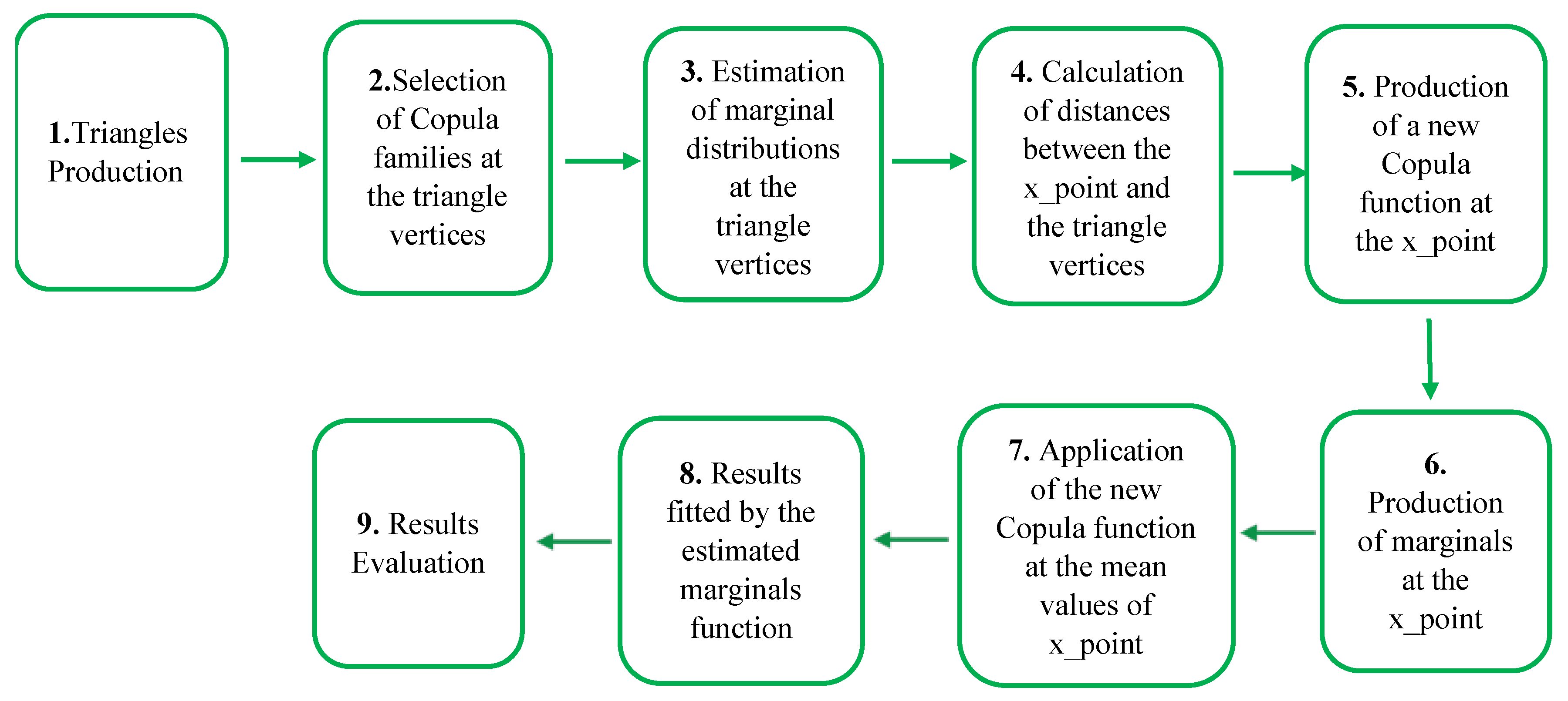
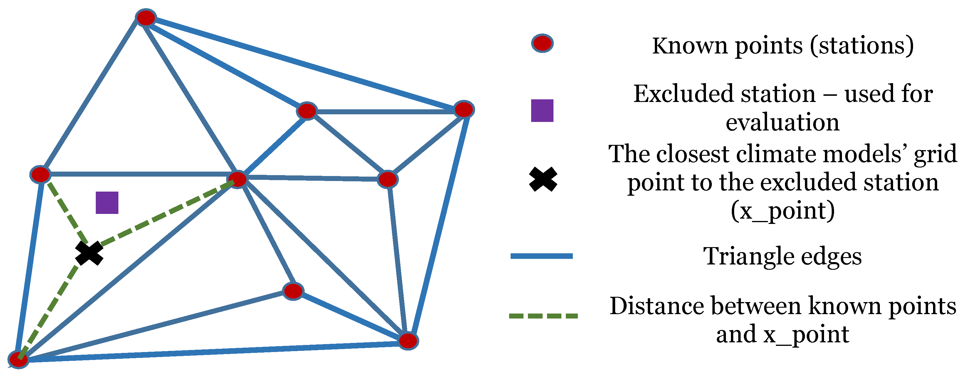
3. Methodology
4. Results
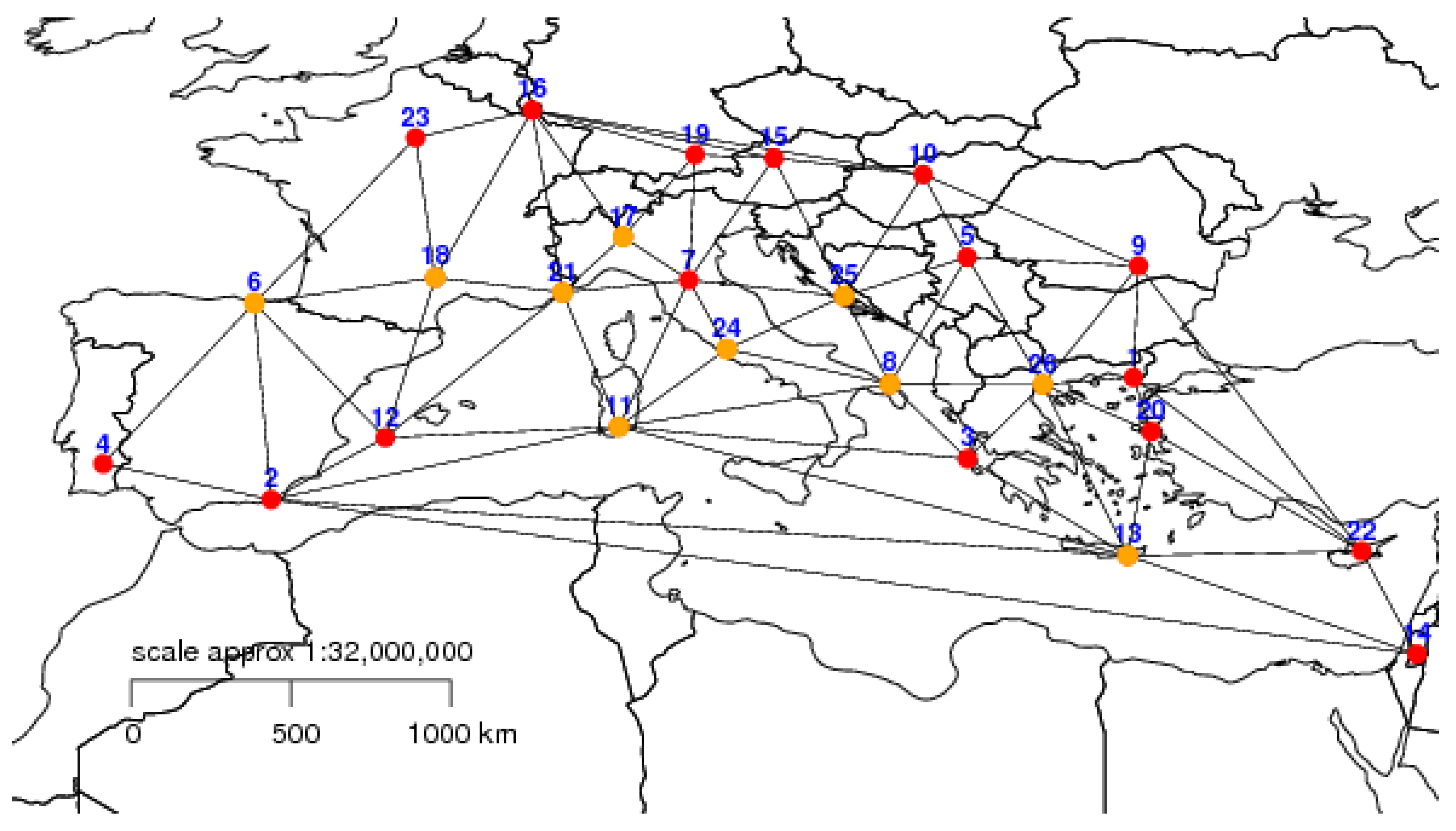
4.1. Selected Stations and Triangles Formation
4.2. Evaluation of the TIN-Copula Method
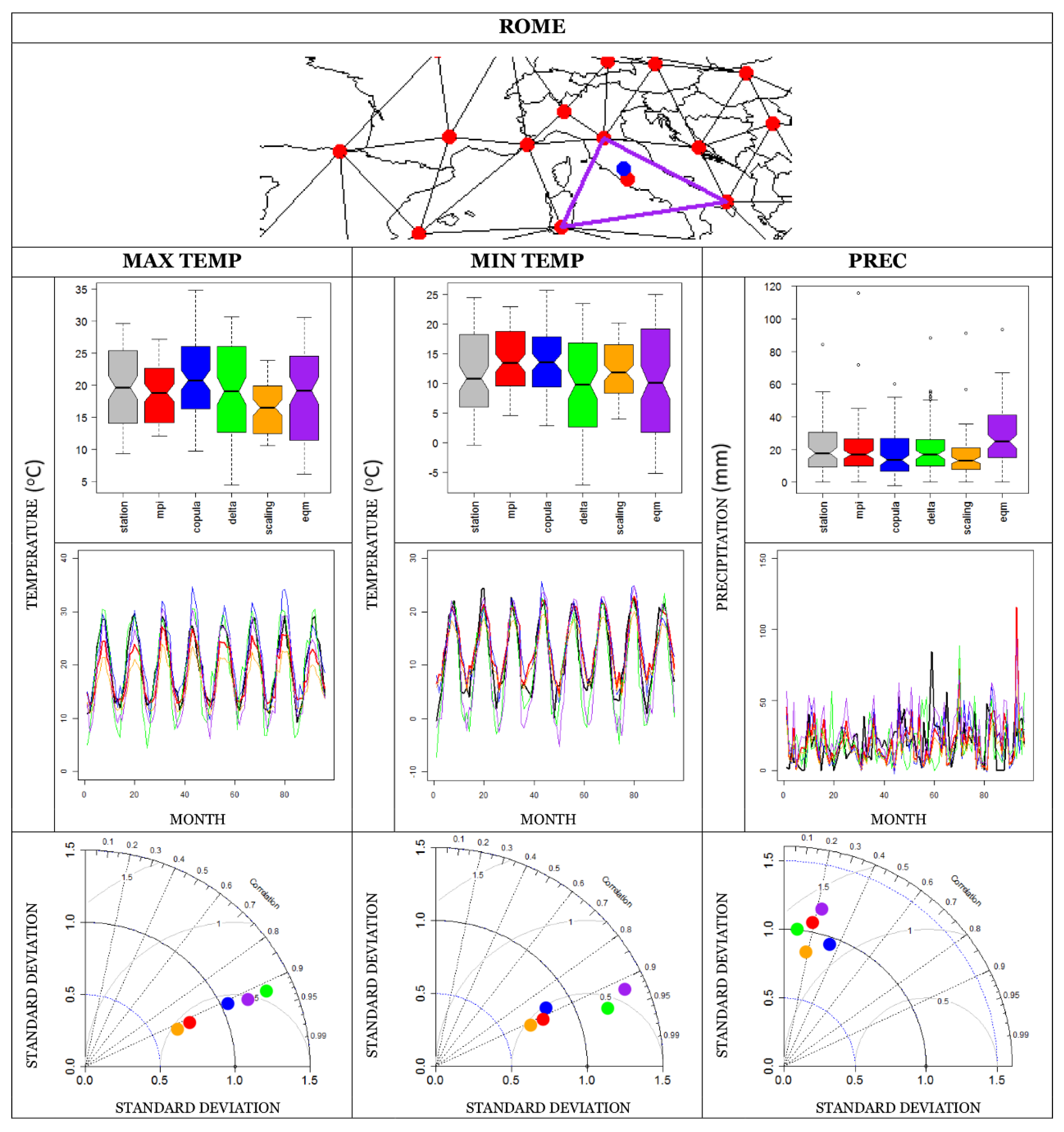
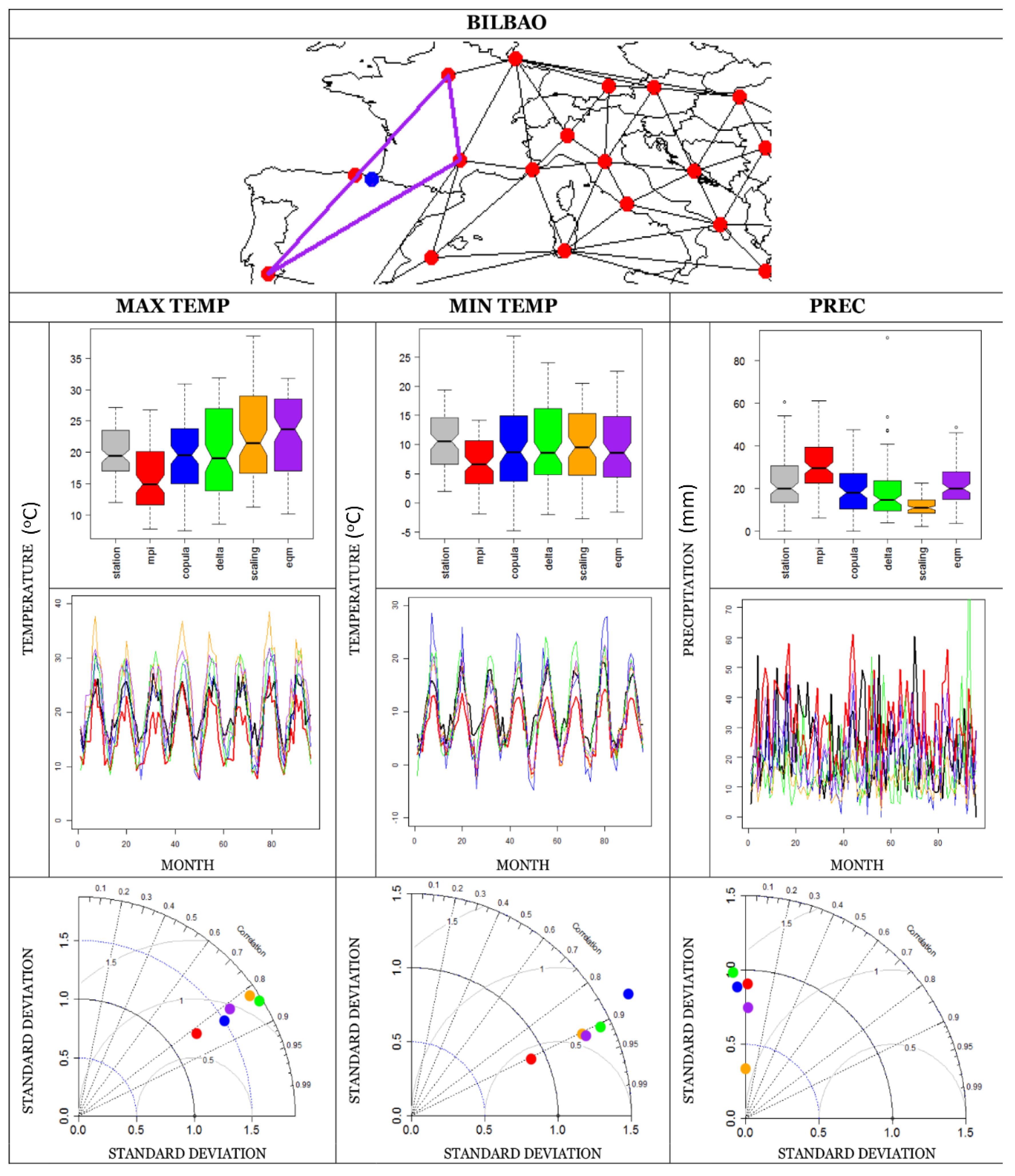
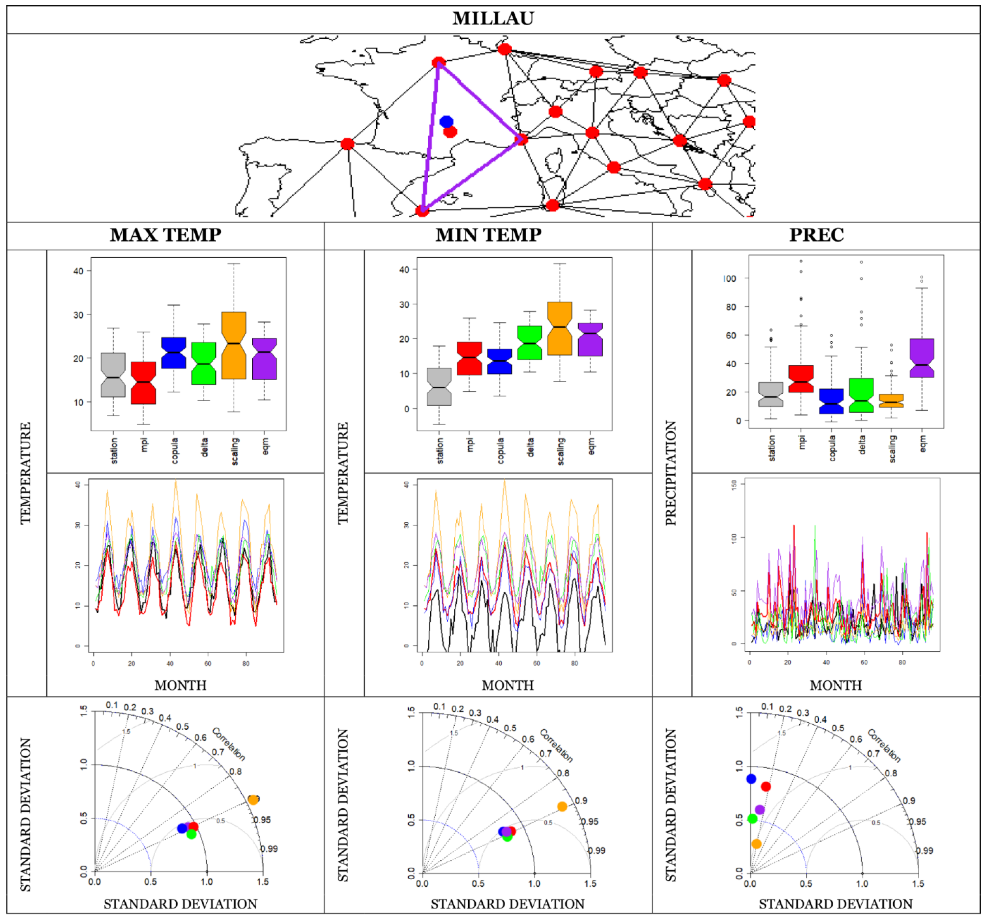
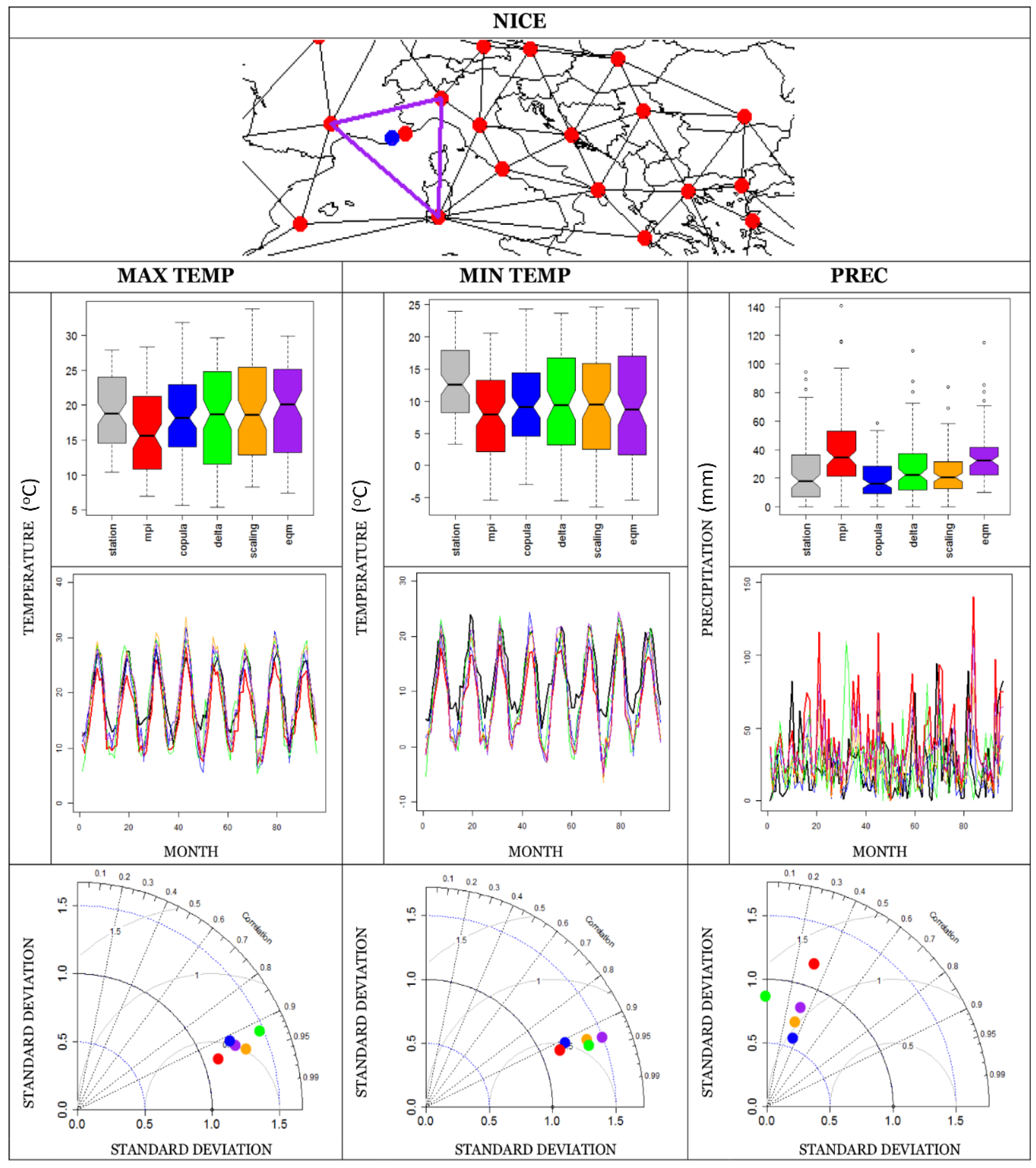
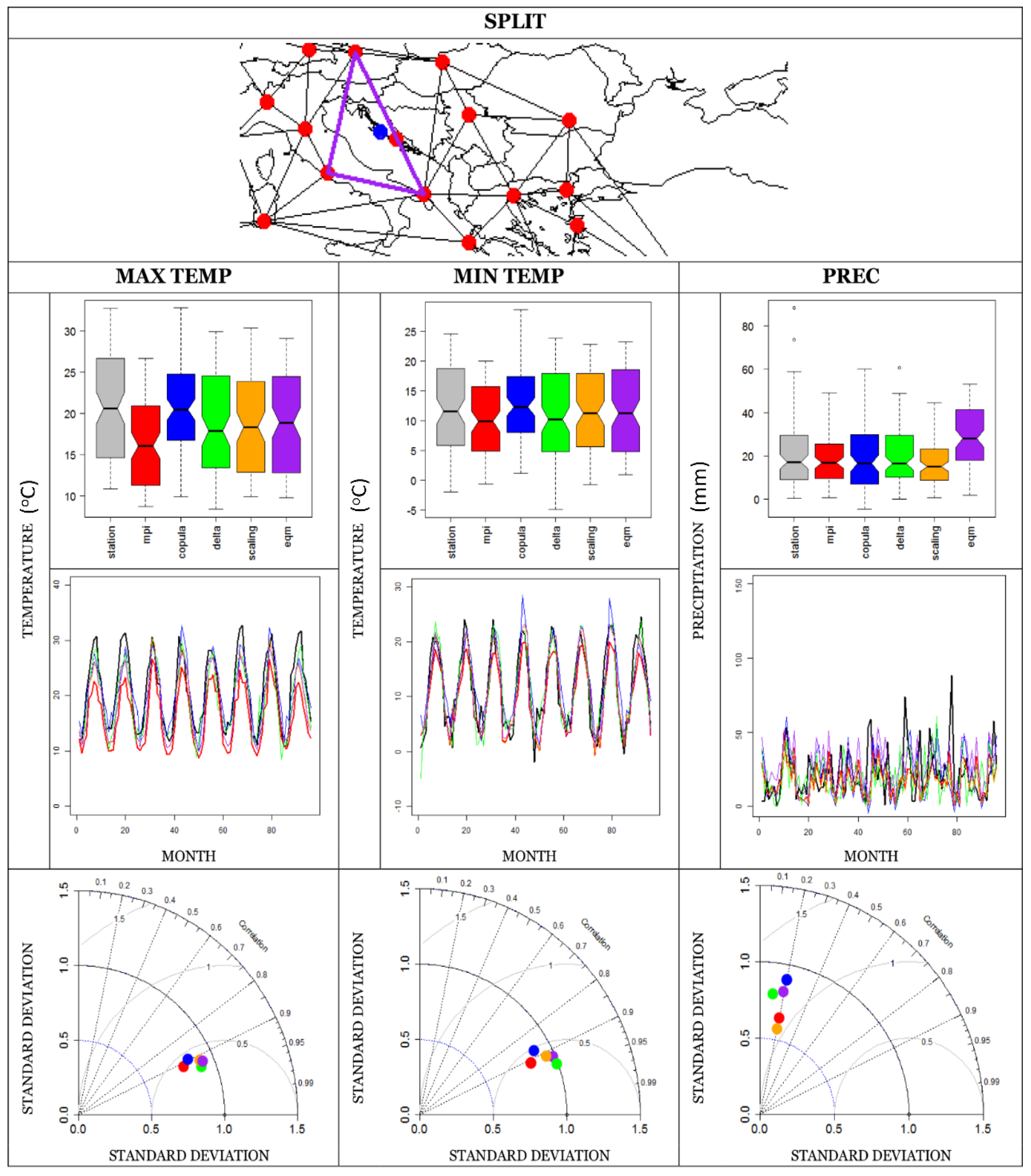
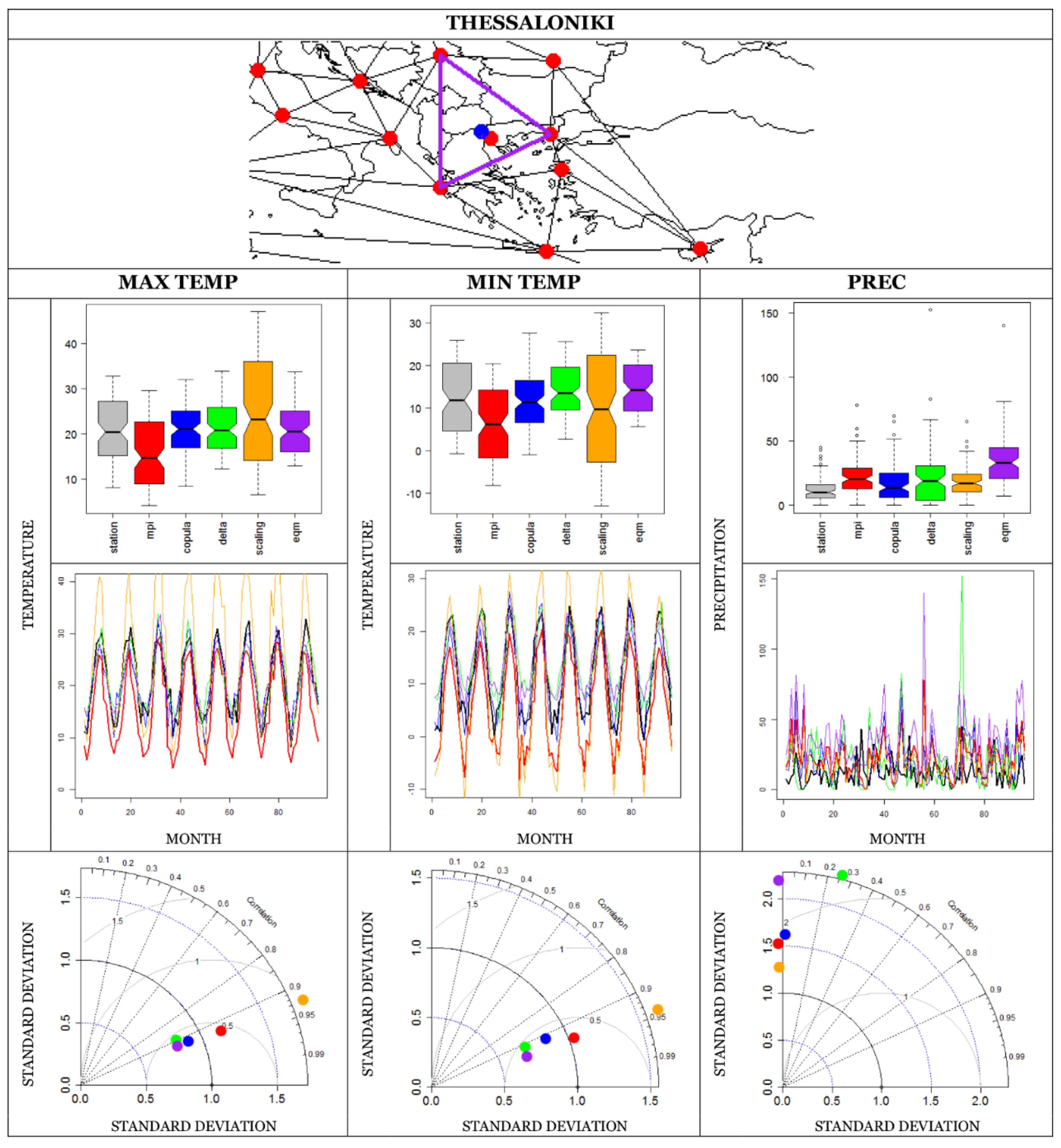
4.2.1. Evaluation with Boxplots-Line Plots and Taylor Graphs
Temperature
Precipitation
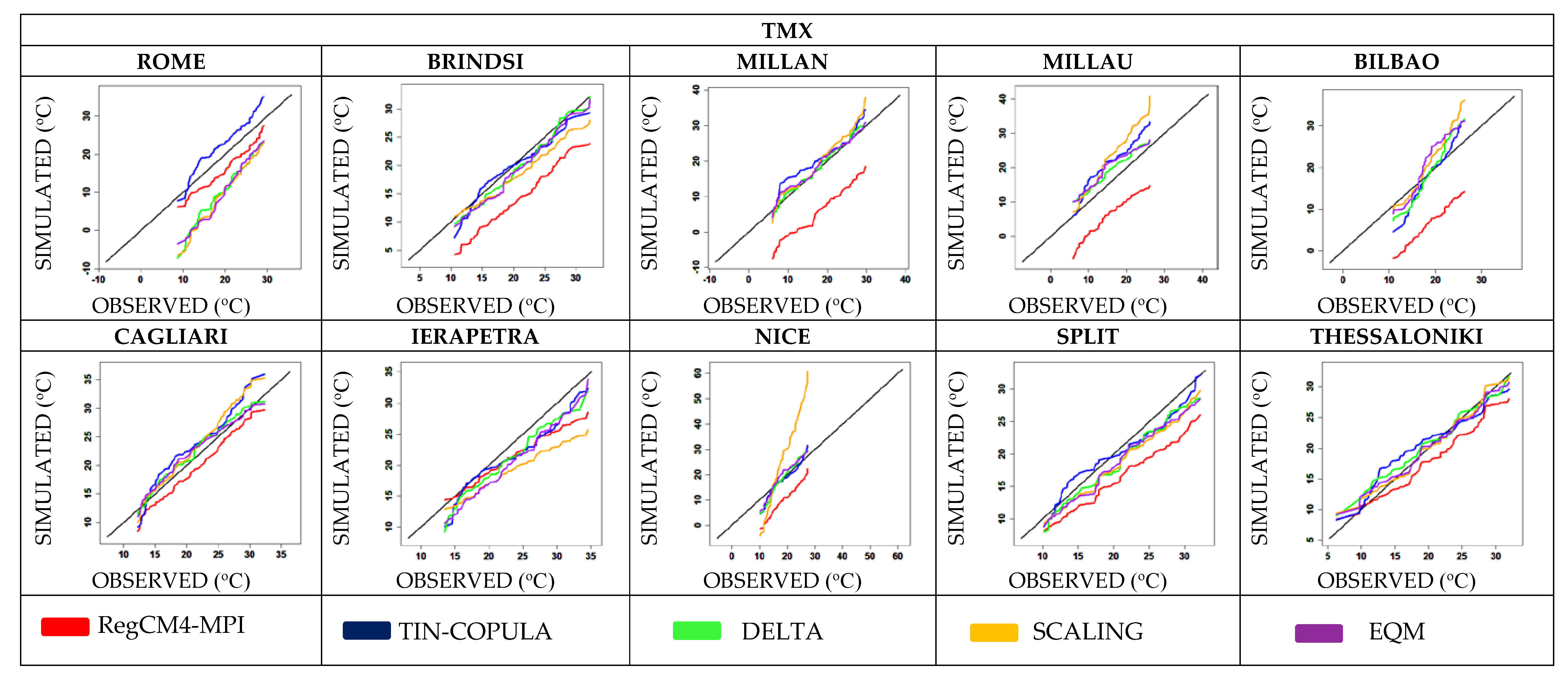
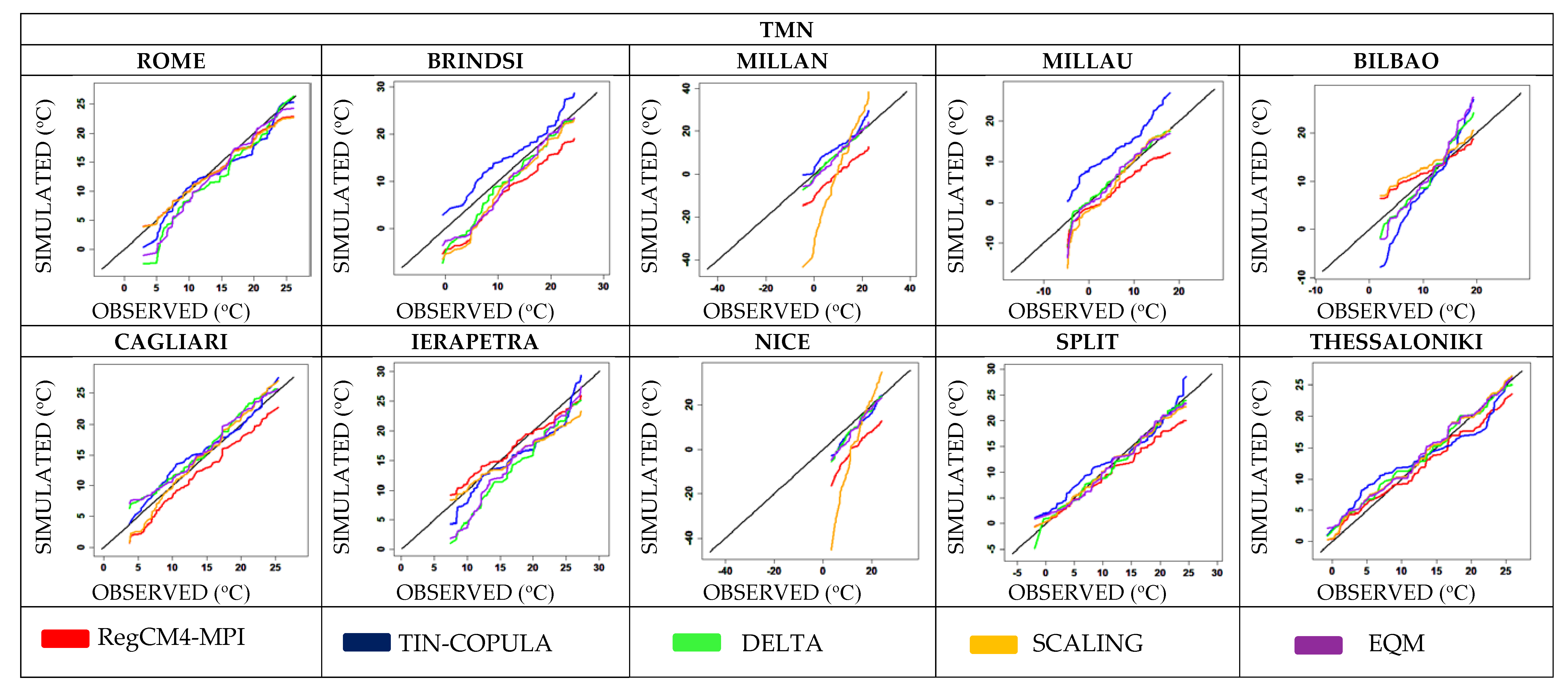
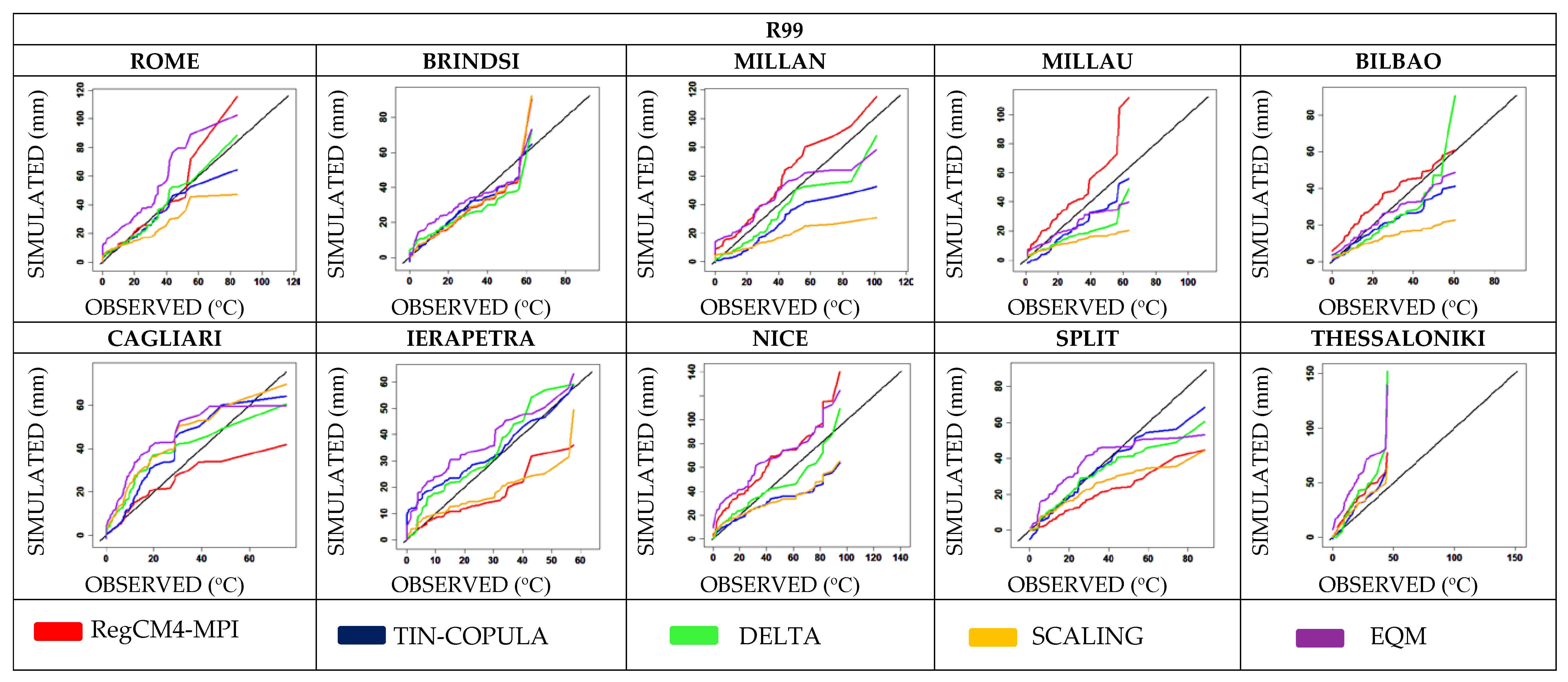
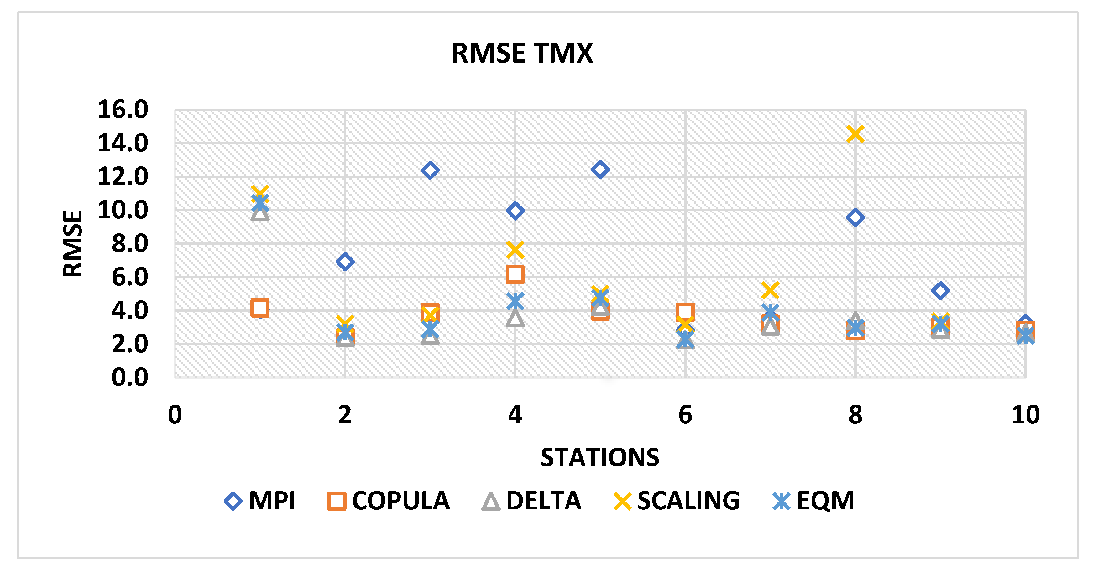
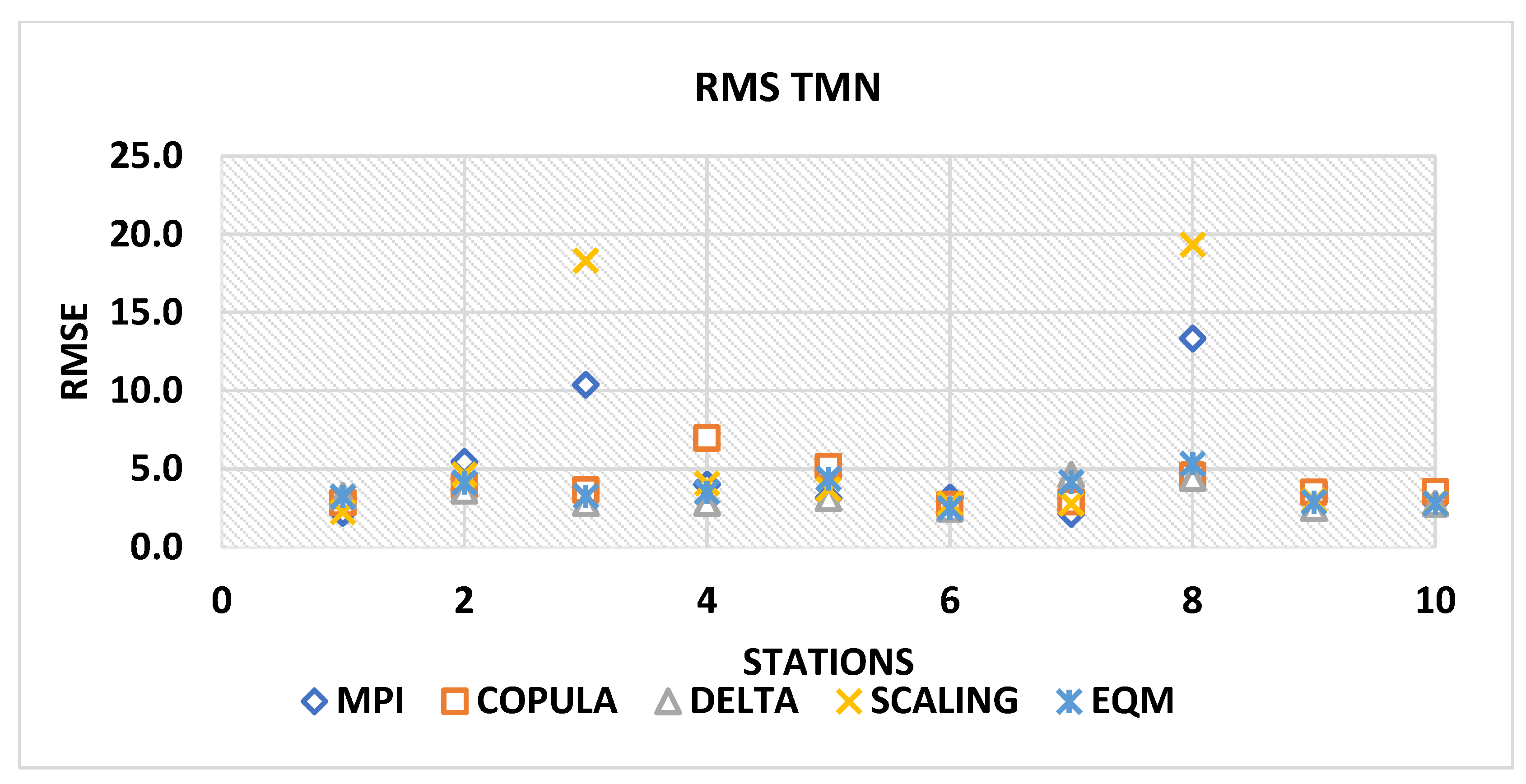
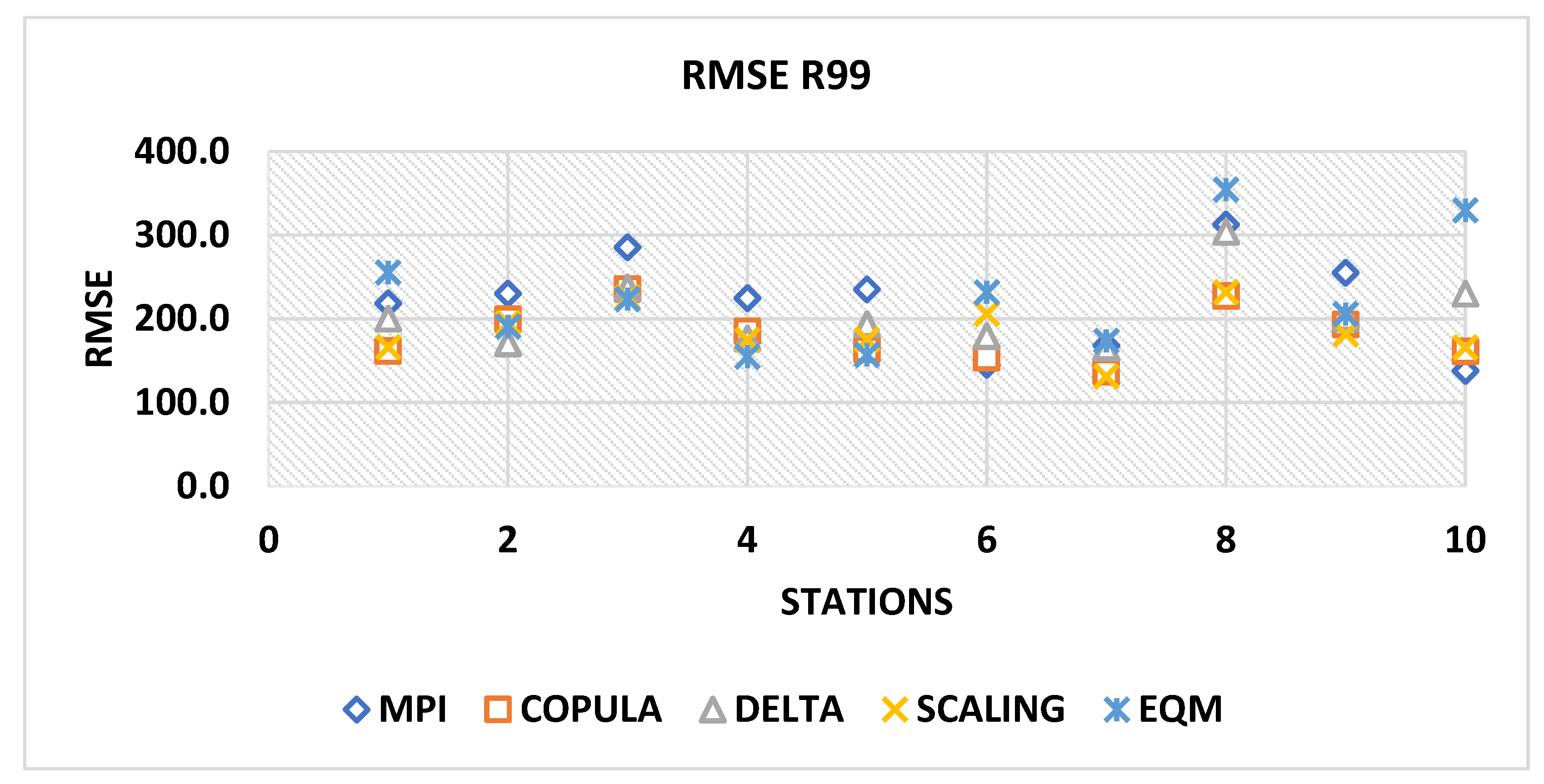
4.2.2. Evaluation with QQ Plots and RMSE Values
5. Discussion and Conclusions
- Firstly, the bias correction with the TIN-copula method can be achieved at every x_point, which is included in a formatted triangle, while the other methods can be applied only at specific points, where observed data exist and used as defaults.
- The second main advantage is that the TIN-copula method uses three neighboring stations for the bias correction of the x-point and not only one as the other methods do. The TIN-copula method and the other methods can present some discouraging results when the climatology of the default station differs importantly from the tested stations. However, the TIN-copula method provides a more robust result, as the three stations can provide better characteristics of the climate of the study region.
- Another advantage of the proposed method is that the whole time period is used, while in the other bias correction methods, sub-time periods are used.
- Additionally, an important advantage of the TIN-copula method is that the estimated new TIN-copula function can be calculated once, meaning that it is unique for each x_point and that it can then be used for different datasets.
- Finally, since in TIN-copula method a specific function is estimated for the studied region, this function is stable also for the future. Consequently, it can be used for the bias correction of the extreme climate model’s values for future periods.
Author Contributions
Funding
Acknowledgments
Conflicts of Interest
Appendix A


References
- World Modeling Summit for Climate Prediction. 2008. Available online: http://wcrp.ipsl.jussieu.fr/Workshops/ModellingSummit/Documents/FinalSummitStat_6_6.pdf (accessed on 15 May 2009).
- Christensen, J.H.; Christensen, O.B. A summary of the PRUDENCE model projections of changes in European climate by the end of this century. Clim. Chang. 2007, 81 (suppl. S1), 7–30. [Google Scholar] [CrossRef]
- Mearns, L.O.; Arritt, R.; Biner, S.; Bukovsky, M.S.; McGinnis, S.; Sain, S.; Caya, D.; Correia, J., Jr.; Flory, D.; Gutowski, W.; et al. The North American Regional Climate Change Assessment Program: Overview of phase I results. Bull. Am. Meteorol. Soc. 2012, 93, 1337–1362. [Google Scholar] [CrossRef]
- Sillmann, J.; Kharin, V.; Zhang, X.; Zwiers, F.; Bronaugh, D. Climate extremes indices in the CMIP5 multimodel ensemble: Part 1. Model evaluation in the present climate. J. Geophys. Res. Atmos. 2013, 118, 1716–1717. [Google Scholar] [CrossRef]
- Sharma, D.; Das Gupta, A.; Babel, M.S. Spatial disaggregation of Bias-corrected GCM precipitation for improved hydrologic simulation: Ping river basin, Thailand. Hydrol. Earth Syst. Sci. 2007, 11, 1373–1390. [Google Scholar] [CrossRef]
- Hansen, J.W.; Challinor, A.; Ines, A.; Wheeler, T.; Moronet, V. Translating forecasts into agricultural terms: Advances and challenges. Clim. Res. 2006, 33, 27–41. [Google Scholar] [CrossRef]
- Johnson, F.; Sharma, A. A nesting model for bias correction of variability at multiple time scales in general circulation model precipitation simulations. Water Resour. Res. 2012, 48, W01504. [Google Scholar] [CrossRef]
- Lafon, T.; Dadson, S.; Buys, G.; Prudhomme, C. Bias correction of daily precipitation simulated by a regional climate model: A comparison of methods. Int. J. Climatol. 2013, 33, 1367–1381. [Google Scholar] [CrossRef]
- Chen, J.; Brissette, F.P.; Chaumont, D.; Braun, M. Finding appropriate bias correction methods in downscaling precipitation for hydrologic impact studies over North America. Water Resour. Res. 2013, 49, 4187–4205. [Google Scholar] [CrossRef]
- Cannon, A.J.; Sobie, S.R.; Murdock, T.Q. Bias correction of GCM precipitation by quantile mapping: How well do methods preserve changes in quantiles and extremes? J. Clim. 2015, 28, 6938–6959. [Google Scholar] [CrossRef]
- Thrasher, B.; Maurer, E.P.; Duffy, P.B.; McKellar, C. Technical Note: Bias correcting climate model simulated daily temperature extremes with quantile mapping. Hydrol. Earth Syst. Sci. 2012, 16, 3309–3314. [Google Scholar] [CrossRef]
- Navarro-Racines, C.E.; Tarapues-Montenegro, J.E.; Ramírez-Villegas, J.A. Bias-correction in the CCAFS-Climate. In Portal: A Description of Methodologies. Decision and Policy Analysis (DAPA) Research Area; International Center for Tropical Agriculture (CIAT): Cali, Colombia, 2015. [Google Scholar]
- Eisner, S.; Voss, F.; Kynast, E. Statistical bias correction of global climate projections–consequences for large scale modeling of flood flows. Adv. Geosci. 2012, 31, 75–82. [Google Scholar] [CrossRef]
- Tabor, K.; Williams, J.W. Globally downscaled climate projections for assessing the conservation impacts of climate change. Ecol. Appl. 2010, 20, 554–565. Available online: http://ccr.aos.wisc.edu/publications/pdfs/globaldownscale.pdf (accessed on 15 August 2015). [CrossRef] [PubMed]
- Xu, Y. Hyfo: Hydrology and Climate Forecasting. R Package Version 1.4.0 2018. Available online: https://CRAN.R-project.org/package=hyfo (accessed on 27 September 2018).
- Hawkins, E.; Osborne, T.M.; Ho, C.K.; Challinor, A.J. Calibration and bias correction of climate projections for crop modelling: An idealised case study over Europe. Agric. For. Meteorol. 2013, 170, 19–31. [Google Scholar] [CrossRef]
- Olsson, J.; Berggren, K.; Olofsson, M.; Viklander, M. Applying climate model precipitation scenarios for urban hydrological assessment: A case study in Kalmar City, Sweden. Atmos. Res. 2009, 92, 364–375. [Google Scholar] [CrossRef]
- Shrestha, M.; Acharya, S.C.; Shrestha, P.K. Bias correction of climate models for hydrological modelling–are simple methods still useful. Meteorol. Appl. 2017, 24, 531–539. [Google Scholar] [CrossRef]
- Ines, A.V.M.; Hansen, J.W. Bias correction of daily GCM rainfall for crop simulation studies. Agric. For. Meteorol. 2006, 138, 44–53. [Google Scholar] [CrossRef]
- Themeßl, M.J.; Gobiet, A.; Heinrich, G. Empirical-statistical downscaling and error correction of daily precipitation from regional climate models. Int. J. Climatol. 2011, 31, 1530–1544. [Google Scholar] [CrossRef]
- Panofsky, H.A.; Brier, G. Some Applications of Statistics to Meteorology; The Pennsylvania State University: Pennsylvania, PA, USA, 1968; p. 224. [Google Scholar]
- Zhang, L.; Singh, V.P. Bivariate rainfall frequency distributions using Archimedean copulas. J. Hydrol. 2007, 332, 93–109. [Google Scholar] [CrossRef]
- Lazoglou, G.; Anagnostopoulou, C.; Skoulikaris, C.; Tolika, K. Bias Correction of Climate Model’s Precipitation Using the Copula Method and Its Application in River Basin Simulation. Water 2019, 11, 600. [Google Scholar] [CrossRef]
- Mao, G.; Vogl, S.; Laux, P.; Wagner, S.; Kunstmann, H. Stochastic bias correction of dynamically downscaled precipitation fields for Germany through Copula-based integration of gridded observation data. Hydrol. Earth Syst. Sci. 2015, 19, 1787–1806. [Google Scholar] [CrossRef]
- Piani, C.; Haerter, J.O. Two dimensional bias correction of temperature and precipitation copulas in climate models. Geophys. Res. Lett. 2012. [Google Scholar] [CrossRef]
- Piani, C.; Haerter, J.O.; Coppola, E. Statistical bias correction for daily precipitation in regional climate models over Europe. Theor. Appl. Climatol. 2010, 99, 187–192. [Google Scholar] [CrossRef]
- Watanabe, S.; Kanae, S.; Seto, S.; Yeh, P.J.F.; Hirabayashi, Y.; Oki, T. Intercomparison of bias-correction methods for monthly temperature and precipitation simulated by multiple climate models. J. Geophys. Res. Atmos. 2012. [Google Scholar] [CrossRef]
- Cannon, A.J. Multivariate quantile mapping bias correction: An N-dimensional probability density function transform for climate model simulations of multiple variables. Clim. Dyn. 2018, 50, 31–49. [Google Scholar] [CrossRef]
- Colette, A.; Vautard, R.; Vrac, M. Regional climate downscaling with prior statistical correction of the global climate forcing. Geophys. Res. Lett. 2012. [Google Scholar] [CrossRef]
- Klein Tank, A.M.G.; Wijngaard, J.B.; Können, G.P.; Böhm, R.; Demarée, G.; Gocheva, A.; Mileta, M.; Pashiardis, S.; Hejkrlik, L.; Kern-Hansen, C.; et al. Daily dataset of 20th-century surface air temperature and precipitation series for the European Climate Assessment. Int. J. Climatol. 2002, 22, 1441–1453. [Google Scholar] [CrossRef]
- Giorgi, F.; Coppola, E.; Solmon, F.; Mariotti, L.; Sylla, M.B.; Bi, X.; Elguindi, N.; Diro, G.T.; Nair, V.S.; Giuliani, G.; et al. RegCM4:model description and preliminary tests over multiple CORDEX domains. Clim. Res. 2012, 52, 7–29. [Google Scholar] [CrossRef]
- Lazoglou, G.; Gräler, B.; Anagnostopoulou, C. Simulation of extreme temperatures using a new method: TIN-copula. Int. J. Climatol. 2019, 39, 5201–5214. [Google Scholar] [CrossRef]
- Peucker, T.K. Some Thoughts on Optimal Mapping and Coding of Surfaces. In Geography and the Properties of Surfaces; Harvard Papers in Theoretical Geography: Cambridge, UK, 1969; pp. 1–11. [Google Scholar]
- Peucker, T.K.; Fowler, R.J.; Little, J.J.; Mark, D.M. Digital Representation of Three-Dimensional Surfaces by Triangulated Irregular Networks (TIN); Technical Report #10; Office of Naval Research (ONR) Geography Programs: Burnaby, BC, Canada, 1977. [Google Scholar]
- Peucker, T.K.; Fowler, R.J.; Little, J.J.; Mark, D.M. The Triangulated Irregular Network. In Proceedings of the Digital Terrain Models (DTM) Symposium, St. Louis, MI, USA, 9–11 May 1978; pp. 516–540. [Google Scholar]
- Delaunay, B. Sur la sphère vide. Bull. Acad. Sci. USSR VII Class. Sci. Mat. Nat. 1934, 7, 793–800. [Google Scholar]
- Akaike, H. Information theory and an extension of the maximum likelihood principle. In Proceedings of the 2nd International Symposium on Information Theory, Tsahkadsor, Armenia, 2–8 September 1971; pp. 267–281. [Google Scholar]
- Schwarz, G. Estimating the dimension of a model. Ann. Stat. 1978, 6, 461–464. [Google Scholar] [CrossRef]
- Ramírez, J.; Jarvis, A. High-Resolution Statistically Downscaled Future Climate Surfaces; International Center for Tropical Agriculture (CIAT); CGIAR Research Program on Climate Change, Agriculture and Food Security (CCAFS): Cali, Colombia, 2008. [Google Scholar]
- Jacob, D.; Bärring, L.; Christensen, O.B.; Christensen, J.H.; De Castro, M.; Deque, M.; Kjellström, E. An inter-comparison of regional climate models for Europe: Model performance in present-day climate. Clim. Chang. 2007, 81, 31–52. [Google Scholar] [CrossRef]
- Christensen, J.H. Regional climate projections, in Climate Change 2007: The Physical Science Basis. In Contribution of Working Group I to the Fourth Assessment Report of the Intergovernmental Panel on Climate Change; Solomon, S., Ed.; Cambridge Univ. Press: Cambridge, UK, 2007. [Google Scholar]


© 2020 by the authors. Licensee MDPI, Basel, Switzerland. This article is an open access article distributed under the terms and conditions of the Creative Commons Attribution (CC BY) license (http://creativecommons.org/licenses/by/4.0/).
Share and Cite
Lazoglou, G.; Angnostopoulou, C.; Tolika, K.; Benedikt, G. Evaluation of a New Statistical Method—TIN-Copula–for the Bias Correction of Climate Models’ Extreme Parameters. Atmosphere 2020, 11, 243. https://doi.org/10.3390/atmos11030243
Lazoglou G, Angnostopoulou C, Tolika K, Benedikt G. Evaluation of a New Statistical Method—TIN-Copula–for the Bias Correction of Climate Models’ Extreme Parameters. Atmosphere. 2020; 11(3):243. https://doi.org/10.3390/atmos11030243
Chicago/Turabian StyleLazoglou, Georgia, Christina Angnostopoulou, Konstantia Tolika, and Gräler Benedikt. 2020. "Evaluation of a New Statistical Method—TIN-Copula–for the Bias Correction of Climate Models’ Extreme Parameters" Atmosphere 11, no. 3: 243. https://doi.org/10.3390/atmos11030243
APA StyleLazoglou, G., Angnostopoulou, C., Tolika, K., & Benedikt, G. (2020). Evaluation of a New Statistical Method—TIN-Copula–for the Bias Correction of Climate Models’ Extreme Parameters. Atmosphere, 11(3), 243. https://doi.org/10.3390/atmos11030243