1. Introduction
Of all the hydrometeorological hazards, floods are the leading cause of fatalities in the United States, based on a National Weather Service (NWS) assessment of 30 years of weather-related fatalities from 1988 to 2017 (
http://www.nws.noaa.gov/os/hazstats.shtml). This ranks floods above tornadoes, derechos, hailstorms, and lightning. Notably, floods not only threaten human lives but also cause extensive damage to property and infrastructure [
1], destruction to crops and loss of livestock [
2], and deterioration of health conditions [
3]. Due to the profound impact of floods on lives and livelihood, it is crucial to understand and forecast precipitation events with sufficient skill to inform the public and stakeholders about expected risks of flood.
As a result of climate change and urbanization, flood statistics are non-stationary [
4]. Theoretical, modeling, and observational research suggests that rainfall rates are increasing [
5,
6,
7] and extreme rainfall events are becoming more frequent [
8,
9,
10]. The most recent report from Intergovernmental Panel on Climate Change (IPCC) finds with high confidence that precipitation over mid-latitude land areas in the Northern Hemisphere has increased since 1951 and predicts that it is “very likely” that extreme precipitation events over mid-latitude land masses will become more intense and more frequent by the end of the 21st century [
11]. Urbanization [
12,
13,
14] and orographic enhancement [
15] may play a critical role in the increased incidence of flooding in certain regions, as well as an increased occurrence of long duration flooding events from both tropical and extratropical cyclones [
16,
17].
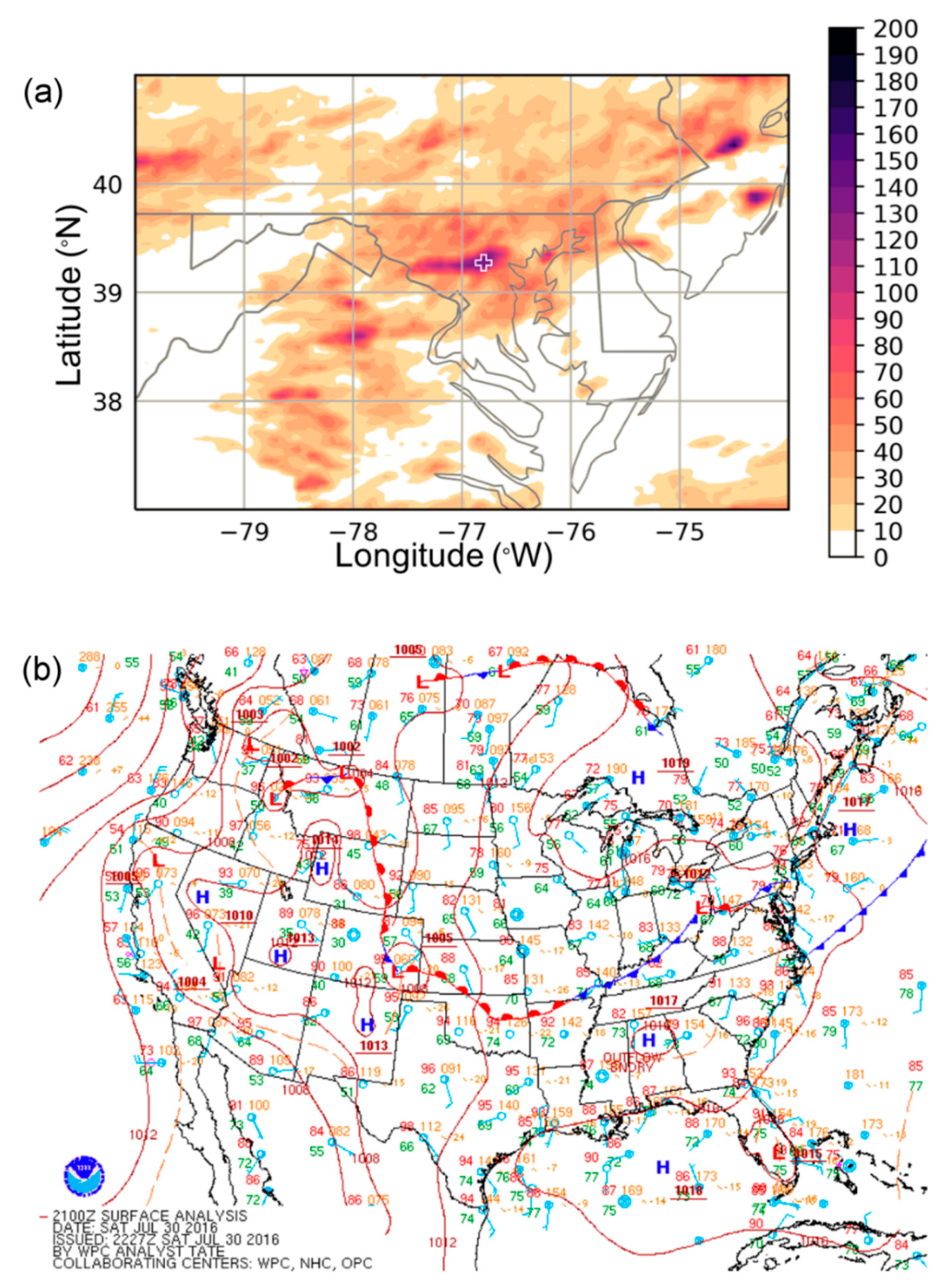
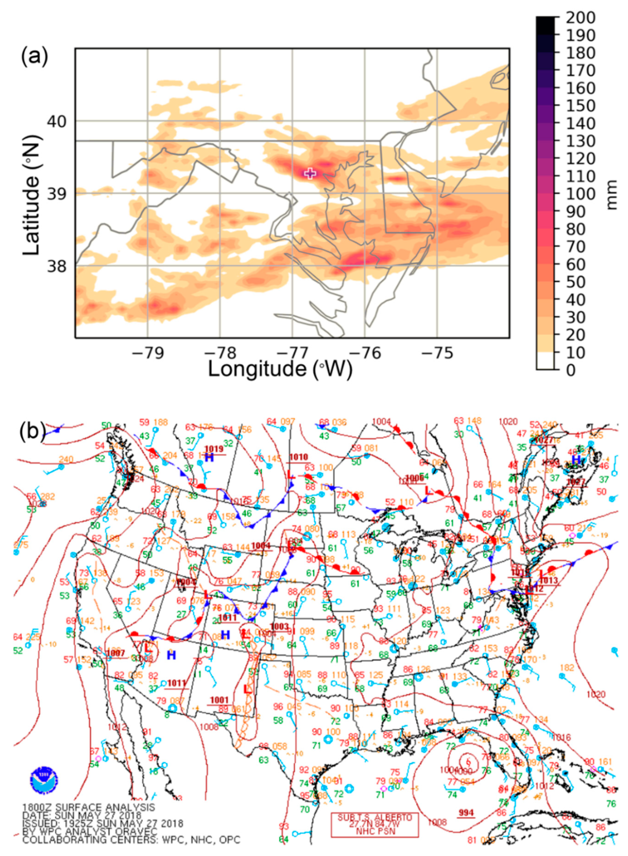
Recent historic floods in Ellicott City, MD, on 30 July 2016 and 27 May 2018 provide stark examples of the types of floods that are expected to become more frequent due to urbanization and climate change. In both cases, rainfall rates exceeded two inches (>50 mm) per hour, leading to an overabundance of run-off, which taxed the city’s storm water infrastructure. The meteorological environments which heralded these two precipitation events were complex, involving the interaction of multiple scales of atmospheric processes that ultimately focused extreme precipitation over Ellicott City and other nearby municipalities to the west of Baltimore, MD. This meteorological set-up resulted in catastrophic rainfall amounts in a short period of time. For a numerical weather prediction (NWP) model to predict these types of events accurately, it must be able to handle dynamical and physical processes over multiple space and time scales. For instance, the synoptic-scale pattern must accurately portray large scale wind and moisture fields in order to forecast the moisture convergence pattern. Frontal and near surface boundaries, which can act as forcings for localized ascent, must also be captured reasonably. At more localized scales, convective and microphysical parameterization schemes must work in conjunction to produce precipitation via sub-grid-scale processes.
Given the expectation of more frequent extreme rainfall events, it is crucial to evaluate the capability of our state-of-the-art NWP models in predicting hydrometeorological events such as the Ellicott City floods. Specifically, to forecast flash flooding, meteorologists (and the model forecasting tools upon which they rely) must be able to predict the evolution of convective-scale (horizontal length scales <10 km) storm elements, which account for the highest rainfall rates [
18]. Additionally, the models need to capture synoptic-scale (horizontal length scales >1000 km) and mesoscale (horizontal length scales between 10 and 1000 km), features that result in training cells or that lead to the development of large, nearly stationary precipitation complexes. Current high-resolution convection-allowing models (CAMs), such as the High-Resolution Rapid Refresh (HRRR) model were developed to capture convective-scale weather phenomena as well as their interaction with larger-scale forcings. In fact, the original release notes from the National Centers for Environmental Prediction (NCEP) stated, “The HRRR provides forecasts, in high detail, of critical weather events such as severe thunderstorms, flash flooding, and localized bands of heavy winter precipitation” [
19]. Yet, as of 2018, only a few studies [
20,
21,
22,
23] have investigated its skill in representing the mesoscale and convective processes that lead to flash flooding.
While there is a lack of research into the specific performance of CAMs in representing extreme precipitation events across multiple scales, there has been abundant research more generally into model skill in predicting precipitation, better known as precipitation verification. Model verification studies provide important information about forecast quality and systematic errors or biases. These studies help end-users in their interpretation of model forecast products and also direct the efforts of researchers in the development of model improvements. Traditional precipitation verification generally fits into one of two categories: visual verification or pixel-based methods. A pixel-based method involves a grid-to-grid comparison between model forecasts and observations from radar, gauge, satellite, or some combination of the above. Using pixel-based methods, users can evaluate summary statistics (e.g., correlations and root-mean-square-error), statistics based on contingency tables (hits, misses, false alarms, and correct negatives) and statistics that derive from contingency tables (probability of detection and various skill scores) (see Wilks [
24] for a comprehensive review).
In recent years, with the rise of high-resolution (horizontal grid spacings ≤4 km) NWP models, there has been increasing interest in new spatial methodologies for precipitation verification. This interest has arisen out of a need to characterize precipitation forecast skill when traditional metrics are hindered by a “double penalty” associated with errors in the timing and/or location of a given precipitation feature [
25,
26]. Several spatial methodologies have been developed. In this study, an object-based approach is utilized, an approach that has become increasingly popular in the research and operational meteorology communities since the development of Contiguous Rain Area [
27] and Method for Object-Based Diagnostic Evaluation [
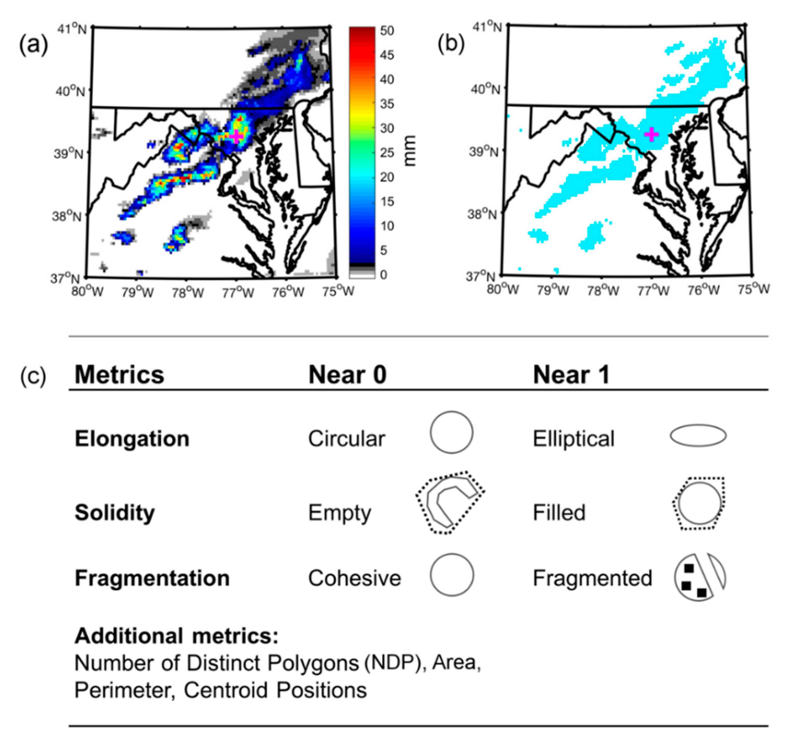
28]. In an object-based approach, precipitation objects, or polygons, are first identified by applying a threshold value to create a binary precipitation field. The polygons are then evaluated for their spatial attributes, which can include location, two-dimensional measures of shape, and average rainfall intensity. Such an objective method is ideal for the present study, since it circumvents the double-penalty problem and also allows for an evaluation of biases with respect to the shape and spatial attributes of the forecast precipitation versus observations.
Due to the nonlinear nature of atmospheric convection, determining an appropriate threshold for delineating a binary precipitation field is a nontrivial subject. In some applications, an ideal method is to delimit a region linked to the fundamental dynamical and physical mechanisms that produce and organize precipitation. For example, Matyas [
29] examined strict 30–40 dBZ reflectivity thresholds (approximately 10 mm h
−1) as the empirically-based separation between stratiform and convective precipitation. However, a lower or higher threshold may be more meaningful to hydrologists and/or emergency managers. Since object-based methods for precipitation verification are sensitive to the threshold value [
30,
31,
32], it is important to evaluate the sensitivity of model forecast skill to the threshold that is specified.
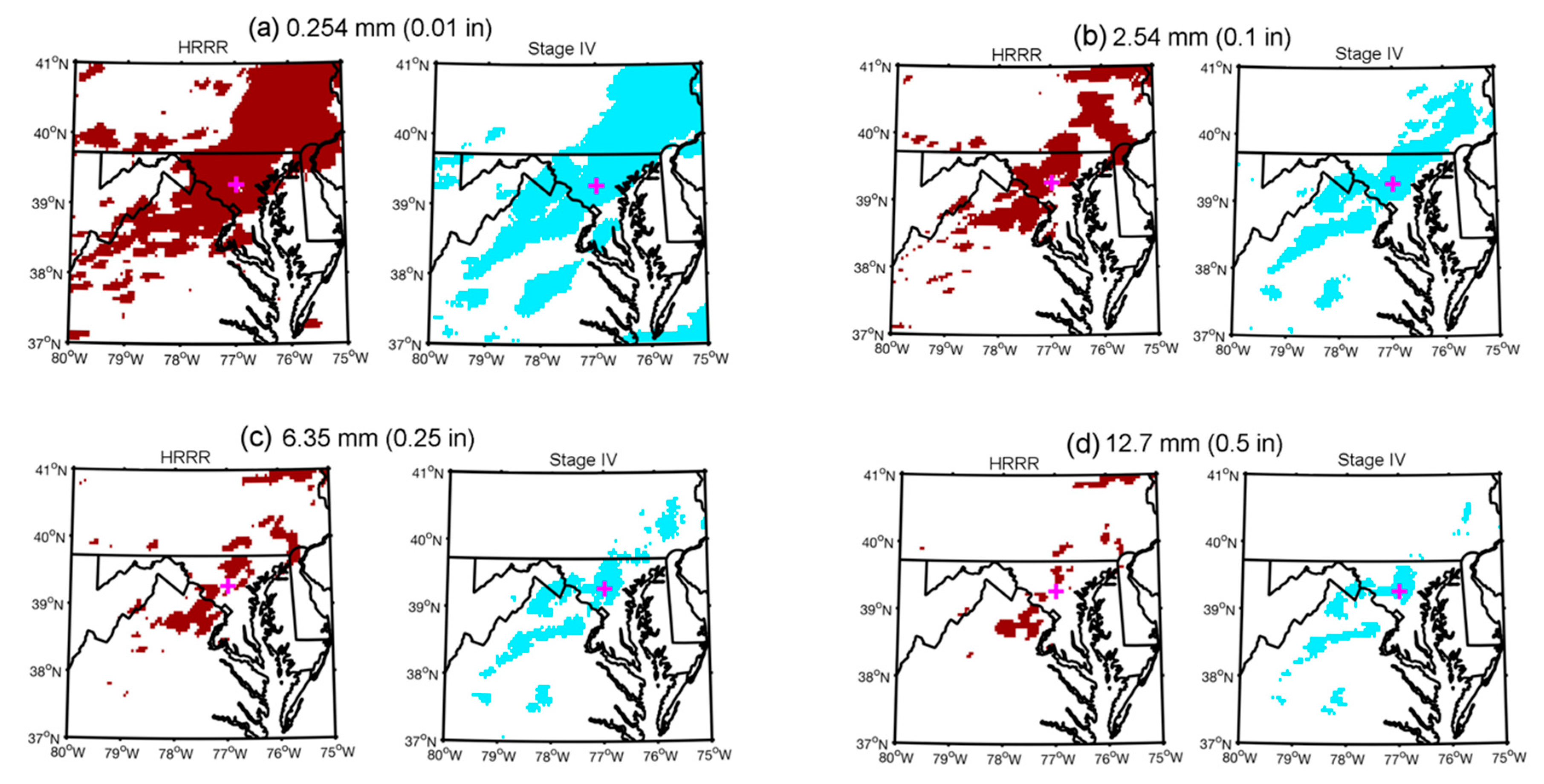
This study utilizes an object-based approach to precipitation verification to quantify HRRR model forecast skill in predicting rainfall in the two aforementioned events that led to catastrophic flooding in Ellicott City and surrounding regions. Two research questions are addressed: (1) can object-based methods offer insight over traditional precipitation verification methods in evaluating NWP skill in predicting these extreme rainfall events? and (2) how does forecast skill vary over a range of rain rate thresholds from “trace” to moderate to extreme precipitation rates? These research questions are evaluated as a proof of concept, and therefore it is important to contextualize the results based on the synoptic and mesoscale environments associated with each event, so as to inform future, more comprehensive studies into high-resolution model precipitation forecast skill.
4. Discussion
The historic rain rates associated with the Ellicott City floods presented a unique opportunity to examine high-resolution NWP skill in predicting extreme rainfall rates. As noted in the introduction, it is expected that anthropogenic climate change will lead to more frequent extreme rainfall events, similar to those evaluated in this study. Because these extreme events severely tax the urban hydraulic infrastructure, it is crucial to assess model skill in characterizing the precipitation forecast. In particular, end users will be interested in understanding model skill at higher rain rate thresholds.
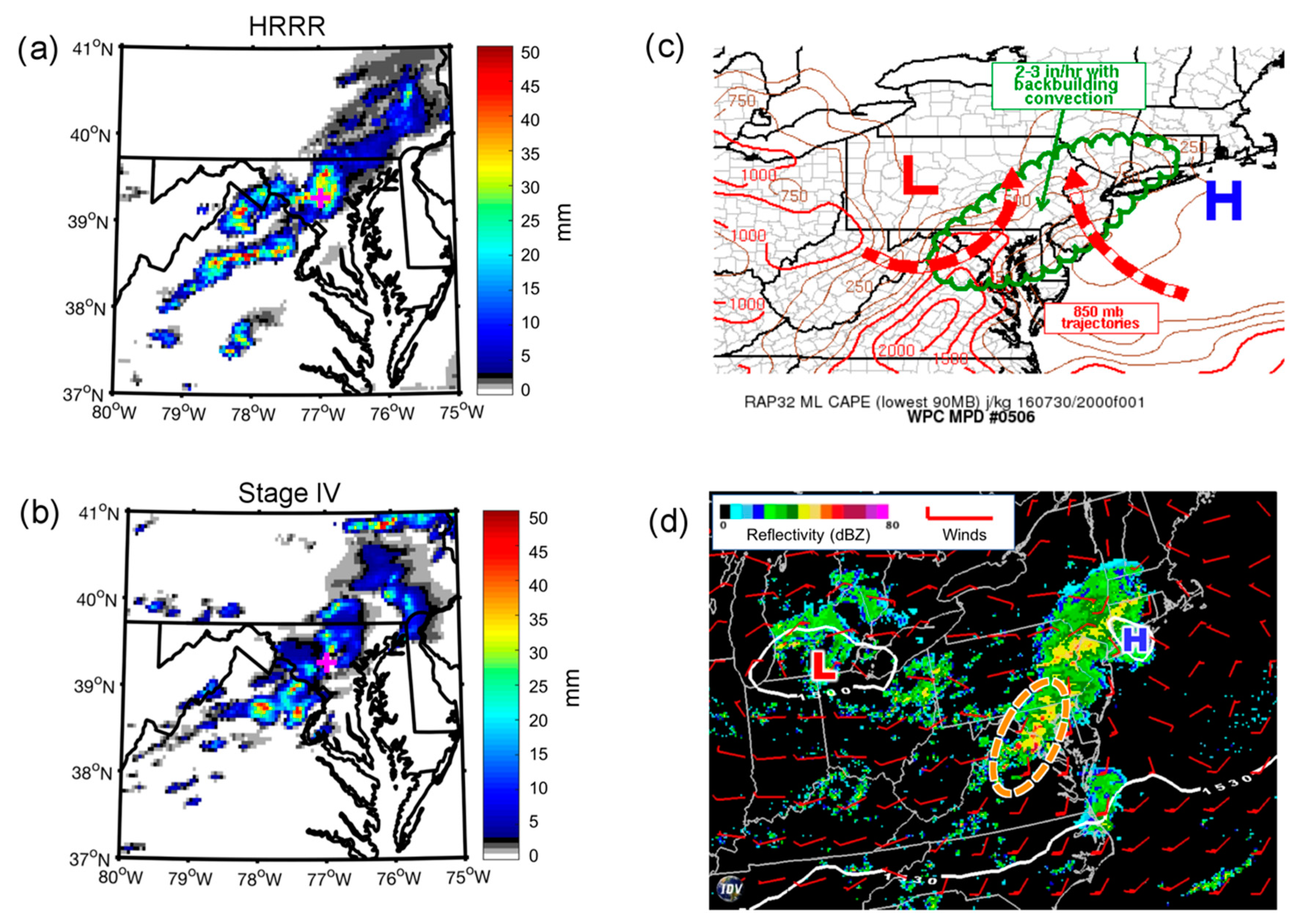
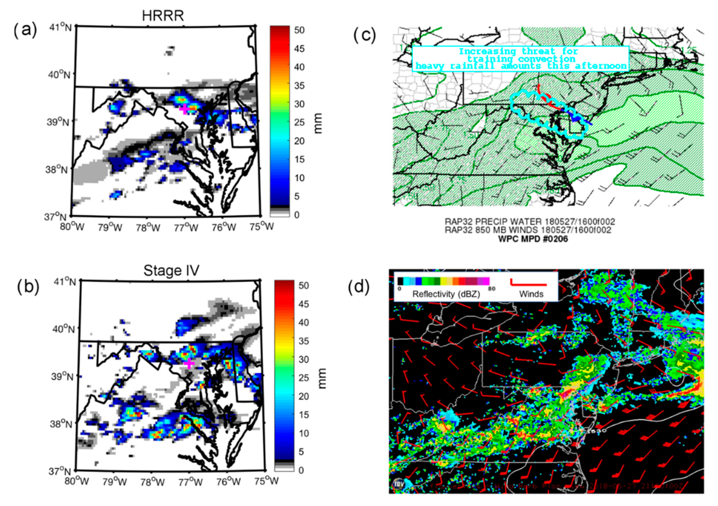
These two case studies highlight that a skillful precipitation forecast requires a skillful representation of synoptic-scale and mesoscale atmospheric processes, such as the large-scale moisture and wind fields and the locations of frontal boundaries. For both case studies, the HRRR model generally provided a good representation of the large-scale environment, and therefore, object-based metrics revealed that there was generally good agreement between model forecast precipitation and observations. However, there important subtle differences between the model and observations in the 2016 event. These subtle differences stress the importance of synoptic-scale and mesoscale processes for both cases. For example, in the first case study, slight differences in the representation of a ridge off the New England coast and the low pressure center over southern Michigan, when compared with the analysis, led to a slight northward displacement of a stationary frontal boundary and, therefore, a displacement of model forecast precipitation to the north of observed precipitation. In the second case study, where synoptic- and mesoscale features were in close agreement between the model and observations, there was no consistent location bias.
Lastly, the two case studies offer some encouraging results for precipitation forecasts at higher rain rate thresholds, in that the models are generally capable of producing rainfall fields that are consistent with observations at these high rain rates. Yet, there is still room for improvement, since model forecasts of extreme convective rainfall tend to be slightly too numerous and fragmented compared with observations. Of note, in the second case study, the highest rainfall rates may have been poorly resolved by the Stage IV observations, which prevented a more in-depth analysis. This highlights the need for improved observational datasets for verification purposes.
Overall, this study provides evidence that should lend confidence to the quality of high-resolution models and the operational forecast products provided to end users. More specifically, this study indicates that high-resolution models, such as the HRRR, can skillfully predict the extreme precipitation rates that are anticipated with anthropogenic climate change. Still, a more comprehensive analysis of systematic biases over a larger sample of extreme precipitation events is necessary to more carefully evaluate HRRR model forecast precipitation. With a better understanding of high-resolution model skill in predicting extreme precipitation events, meteorologists and emergency managers can work together more effectively to save lives when flash floods threaten communities.
5. Conclusions
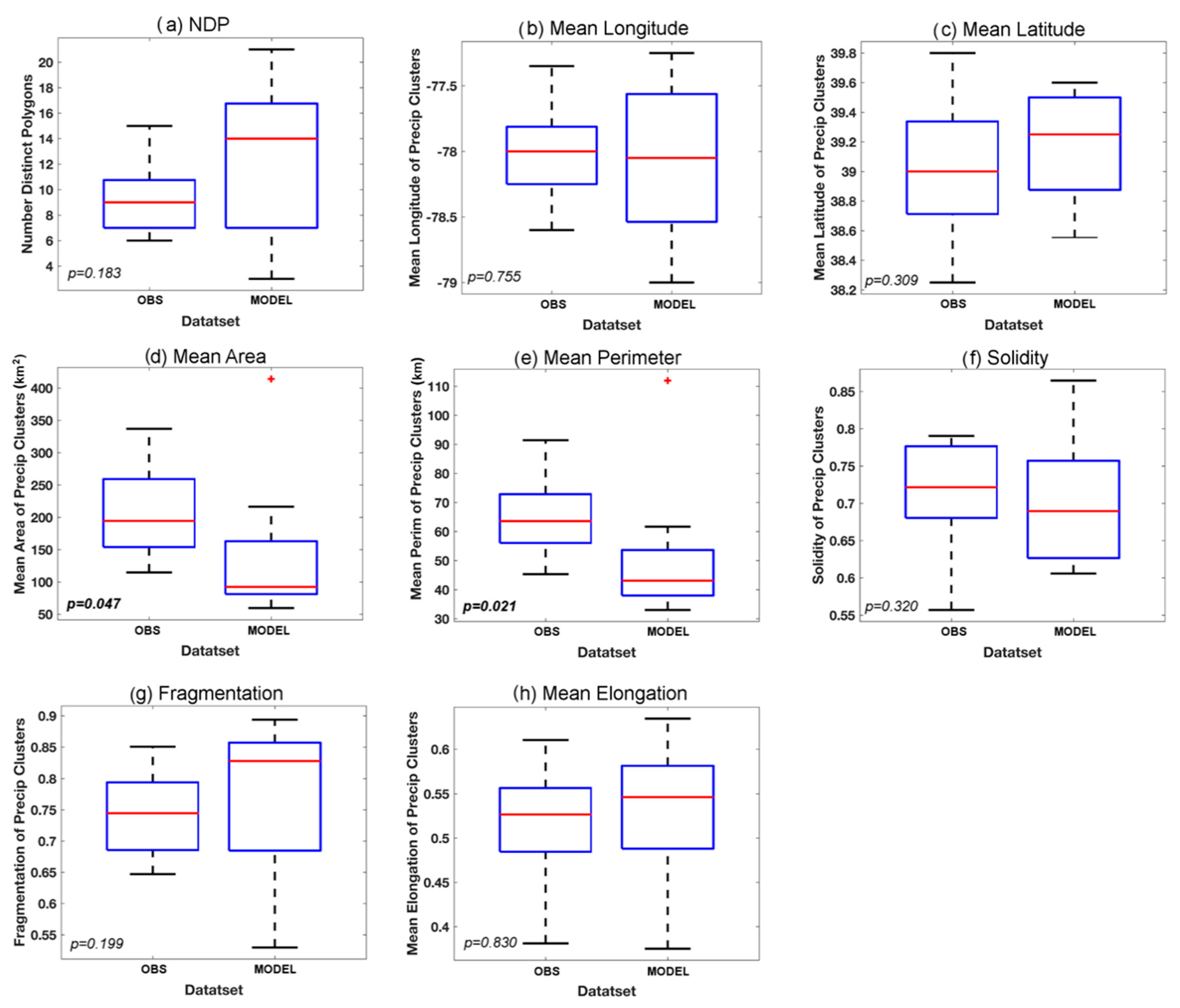
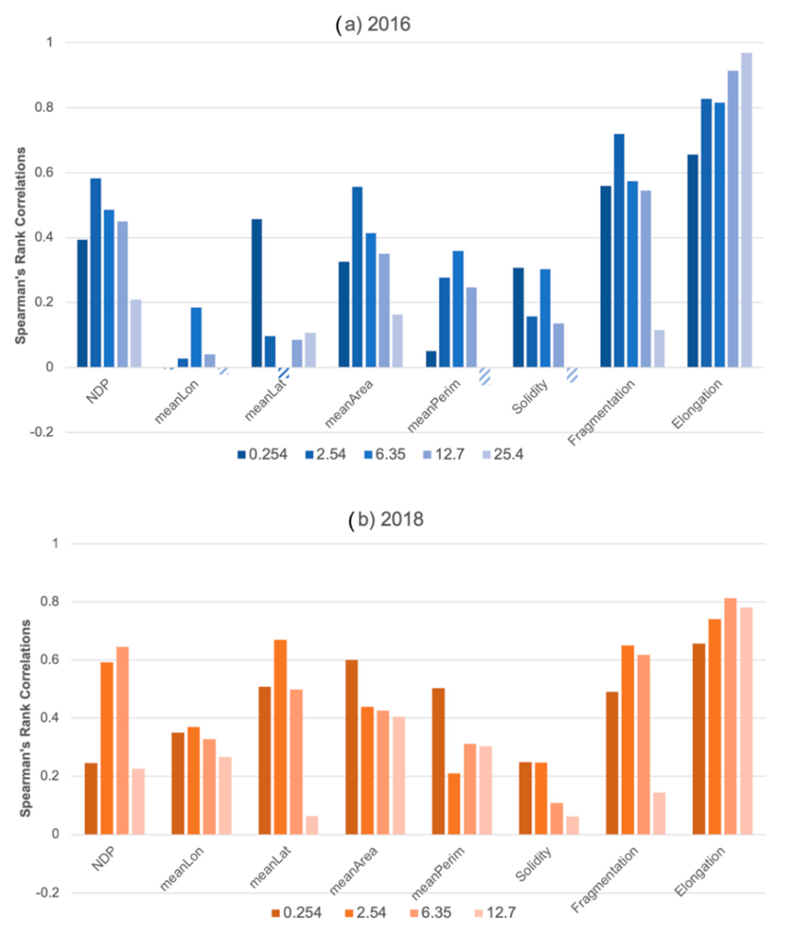
This study used an object-based method to evaluate hourly precipitation forecasts from the HRRR model against Stage IV observations during two high-impact flash flooding events in Ellicott City, MD. Spatial metrics were utilized to quantify the spatial attributes of precipitation features. A Mann–Whitney U-test then revealed systematic biases (using a confidence level of 90%) related to the shape and location of model forecast precipitation. Additionally, model forecast skill was evaluated over a range of rain rates that span stratiform and convective precipitation regimes.
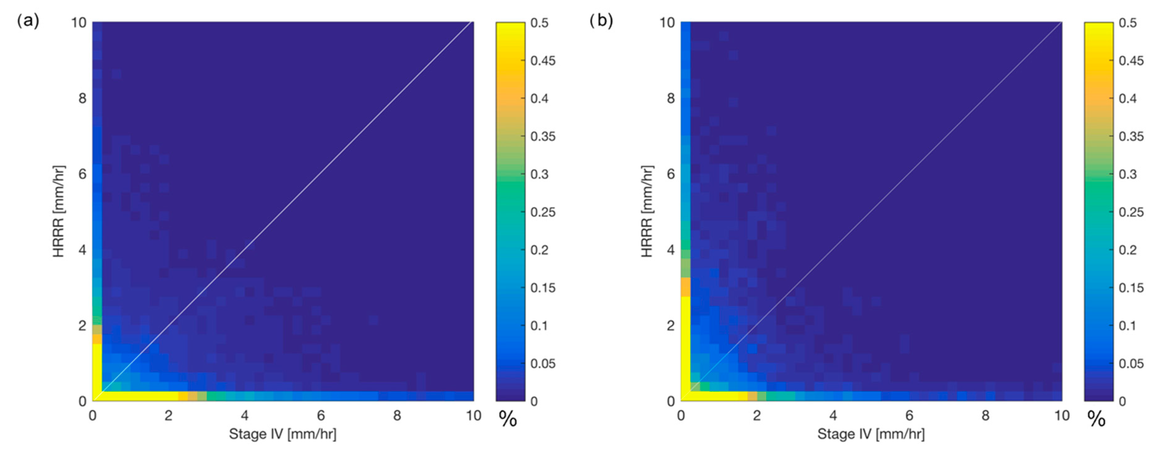
Results indicated that traditional pixel-based precipitation verification metrics, such as those based on two-dimensional histograms, are limited in their ability to quantify and characterize model skill, due in large part to location differences in the location of precipitation. An object-based approach provided additional useful information model biases with respect to location and spatial structure of the forecast precipitation field.
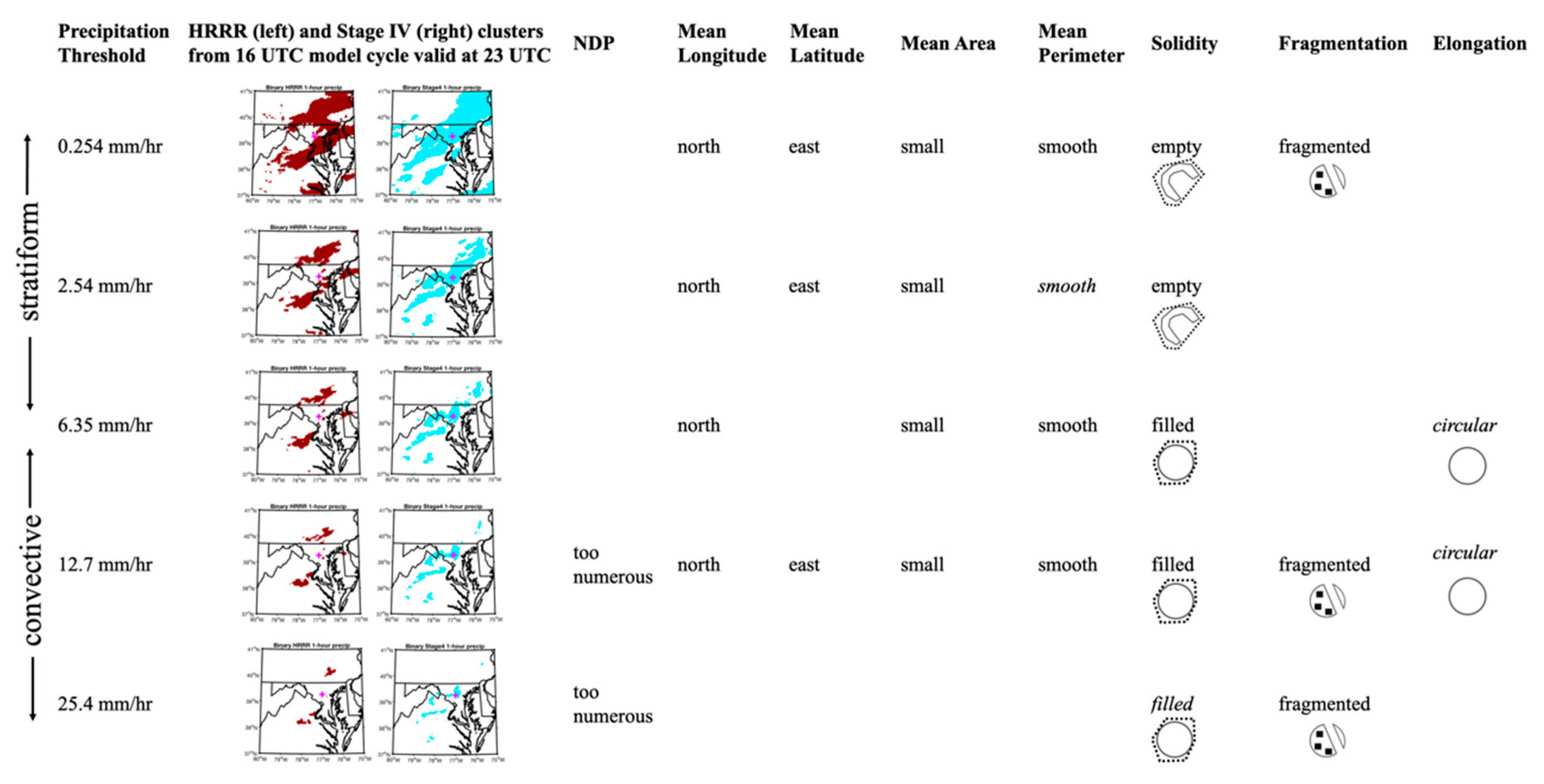
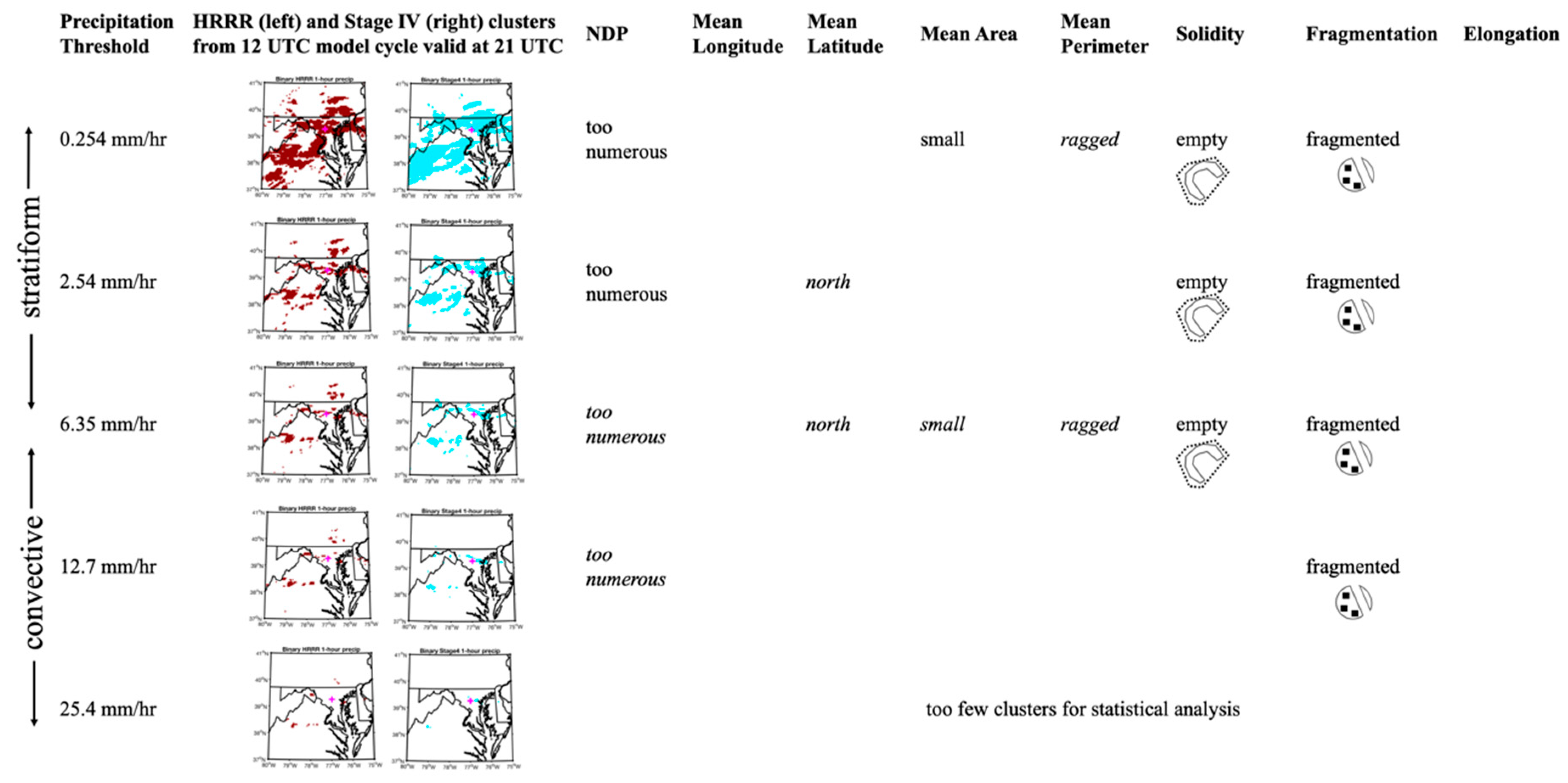
An important objective of this research was to evaluate model skill over multiple rain rate thresholds. In this limited study based on two cases, the results indicated that model skill was sensitive to rain rate threshold. Yet, the results were also sensitive to the case under consideration, which led to some inconsistencies in the results from the two studies that may indicate that the biases that were observed in one case study may not be systematic to the model. For instance, a location error was only observed in the July 2016 flood, with a slight bias for the model to forecast precipitation at the lower rain rate thresholds to the northeast of the observed locations. No location bias was present at higher rain rate thresholds or for the May 2018 flood. A more consistent issue across both case studies was a tendency for the model to predict a precipitation field that was too fragmented compared with the observations. This bias toward a fragmented precipitation field was present across all thresholds, but most particularly at low rain rate (<5 mm h−1) and high rain rate (>10 mm h−1) thresholds. Lastly, the model tended to over-forecast the number of polygons associated with high rain rate thresholds, which contributed to the high fragmentation bias. Interestingly, moderate rain rate (5–10 mm h−1) regions in the 2016 flood were one major exception to an otherwise consistent high fragmentation bias: at the 6.35 mm h−1 threshold, the polygons tends to be too cellular (solid with smooth edges).
Overall, the results indicate that the HRRR forecast showed some skill in predicting a potential for extreme rainfall in both of the Ellicott City floods, though the model tended to overpredict the rainfall rates in the 2018 flood versus observations. Here, it is important to note that the 4 km Stage IV dataset may have struggled with resolving the high rain rates that were observed over a small area in this more isolated precipitation event. Still, the object-based approach revealed a tendency to overpredict the number of high rain rate regions.
Both case studies stressed that an accurate forecast of the synoptic and mesoscale environment was crucial to precipitation forecast skill across all rain rate thresholds. For example, the HRRR model struggled more with the synoptic-scale environment in the 2016 case, where a weak high pressure was present to the northeast of the study area. With a region of low pressure over southern Michigan and that high pressure off the New England coast, there was a region of convergence over central Maryland, which promoted the development of backbuilding convection over the Ellicott City area. In the 12 UTC model cycle and in model cycles closely preceding the event, these features were forecast with better skill, and the resulting forecast of convective-scale elements also verified better with the observations. Furthermore, the northeast bias in the location of convection was also related to the representation of these synoptic- and mesoscale weather features. In the 2018 case study, the southerly flow, ample moisture transport, and location of stationary front were more consistently forecast across all model cycles, leading to slightly better skill with respect to the object-based metrics, including a better forecast with respect to the location of precipitation. Overall, the object-based metrics offer evidence that the models are capable of producing extreme precipitation but also that the location and characteristics of that precipitation depend on accurate depiction of synoptic- and mesoscale weather features. These results support that a detailed surface analyses [
60] and an “ingredients-based” approach [
61] should remain central to the process of forecasting excessive rainfall.
This paper presents two case studies of extreme precipitation events that led to flash flooding in Ellicott City, MD, and therefore there are limitations that arise due to the selection of the cases and the small sample size. A more comprehensive study needs to be performed to evaluate high-resolution precipitation forecasts for such extreme precipitation events. Additionally, future studies need to evaluate precipitation forecast skill over a comprehensive set of synoptic and mesoscale environments to better understand how skill varies by large-scale forcing and storm mode (e.g., linear frontal systems versus isolated cellular storms). Additionally, this study analyzed the model skill over the evolution of the event. An alternate approach would be to utilize a time-lagged ensemble or the new experimental HRRR ensemble to evaluate model skill at individual forecast (valid) times. Lastly, the spatial metrics utilized in this study do not necessarily represent a comprehensive set of independent spatial metrics. More work needs to be conducted to identify the most relevant metrics that capture the diverse range of two-dimensional rainfall patterns associated with mesoscale convection. Thus, this study represents a stepping stone toward a comprehensive evaluation of precipitation in high-resolution forecast models.


