Article

Quantifying the Independent Influences of Land Cover and Humidity on Microscale Urban Air Temperature Variation in Hot Summer: Methods of Path Analysis and Genetic SVR

College of Resources and Environment, Huazhong Agricultural University, Wuhan 430070, China
*
Author to whom correspondence should be addressed.
Atmosphere 2020, 11(12), 1377; https://doi.org/10.3390/atmos11121377
Submission received: 6 December 2020 / Revised: 15 December 2020 / Accepted: 16 December 2020 / Published: 21 December 2020

Abstract

:
Mitigating high air temperatures and heat waves is vital for decreasing air pollution and protecting public health. To improve understanding of microscale urban air temperature variation, this paper performed measurements of air temperature and relative humidity in a field of Wuhan City in the afternoon of hot summer days, and used path analysis and genetic support vector regression (SVR) to quantify the independent influences of land cover and humidity on air temperature variation. The path analysis shows that most effect of the land cover is mediated through relative humidity difference, more than four times as much as the direct effect, and that the direct effect of relative humidity difference is nearly six times that of land cover, even larger than the total effect of the land cover. The SVR simulation illustrates that land cover and relative humidity independently contribute 16.3% and 83.7%, on average, to the rise of the air temperature over the land without vegetation in the study site. An alternative strategy of increasing the humidity artificially is proposed to reduce high air temperatures in urban areas. The study would provide scientific support for the regulation of the microclimate and the mitigation of the high air temperature in urban areas.

1. Introduction

High air temperatures and heat waves, which alter the air physicochemical process and then increase air pollution [1,2], exert severe impacts on both the environment and public health. Many studies have reported that high air temperatures and heat waves are associated with mortality risks and substantial illnesses around the world [3,4,5,6,7,8,9,10]. With the background of global warming [11,12] and heat waves increasing in frequency and intensity [13,14], the global and the regional increases in air temperature continually and increasingly receive special attention from the public and academics [15,16]. As urbanization continues, mitigating high air temperatures and heat risks is a vital challenge for the sustainable development of cities [17], as well as for sustainable development of human society as a whole.
Although it has gradually become a common view that the increase in concentrations of greenhouse gases, which trap outgoing long-wave radiation from the Earth to space, is an influential factor leading to the increase in global air temperature [12,18,19], there is a growing consensus that land cover variation exhibits more local effects on air temperature rather than the global effects produced by greenhouse gas emissions [20,21]. The change of land cover directly modifies the energy budget and the matter exchange with the atmosphere, and also modifies the circulation of the atmosphere near the land surface, thereby inducing the variation of the local and regional air temperature and leading to the modification of the microclimate [22,23,24]. This effect, in some cases caused by processes such as deforestation, agricultural practices, and urbanization, may even exceed the effect of greenhouse gases [25,26].
Taking into account the replacements of natural land cover in the city, the increase in urban vegetation is often a recommended strategy for cooling urban areas and mitigating high air temperatures [27,28,29]. However, increasing vegetation is usually accompanied with an increase in humidity [30,31]. It is difficult to distinguish between the contributions of vegetation and humidity increases to temperature decreases. A key process of vegetation affecting air temperature is evapotranspiration, the loss of water from a plant as a vapor into the atmosphere, which consumes surface energy and increases latent heat, cooling the ambient air temperature. Similarly, higher humidity might lead to dissipation of more of the surface energy as latent heat flux, thereby decreasing the air temperature. According to the energy budget model [32], latent heat flux is proportional to the specific humidity gradient in the vertical direction. Thus, the humidity may also have an important influence on urban air temperature variation. Thereafter, water-based technologies, such as water sprays and fountains, are also proposed to mitigate urban heat and improve thermal comfort through experimental and numerical studies [33,34,35]. Moreover, the effects of water sprays and fountains are especially significant in cities which are characterized by a high urban density with a low percentage of green areas [36]. In addition, these technologies have been implemented to create pedestrian cool spots during international exhibitions in cities such as Osaka, Seville, Aichi, and Shanghai [37]. Additionally, previous studies have shown that urban heat island (UHI) changes were negatively related to humidity variation, with higher UHIs in lower humidity areas [38,39].
Although the effects of land cover and humidity on air temperature are recognized, the relative magnitude of their influences remains inadequately uncovered, and quantifying the independent contributions of these two factors to the variation of air temperature has received less attention. To improve understanding of microscale air temperature variation in urban areas, we attempt to quantify the independent influences of land cover and humidity on variation of air temperature in hot summer. We conducted air temperature and relative humidity measurements in a field containing two different types of land cover in Wuhan city, China, in the afternoons of hot summer days. We then conducted a path analysis to examine the effects of the land cover and the humidity difference impacting on air temperature differences, with the purpose of quantifying the direct and indirect causal contribution of them. Furthermore, we used support vector regression (SVR), which was combined with a genetic algorithm (GA) to obtain optimal parameters, to fit the relationship of air temperature differences with these two factors. Afterward, we simulated the independent contributions of the two factors to air temperature differences. The direct and indirect links between these two factors and air temperature differences, combined with individual contribution analysis, would provide sound information for urban heat adaptation. The efforts of this work are intended to serve for the microclimate regulation and potential strategies to mitigate high air temperatures and heat waves in urban areas.

2. Materials and Methods

2.1. Field Measurements

Our study site is located at latitude 30°28′30″ and longitude 114°21′27″, in Hongshan District, Wuhan, China. Wuhan, the capital of Hubei Province, is a city with the largest population in Central China. The city has a humid subtropical climate with abundant rainfall, cool winters, and hot summers, and its average elevation is about 37 m above sea level. As one of the Four Furnaces of China, Wuhan is always suffering heat waves and high air temperatures in the summertime. The study site is a flat field consisting of a plot of bush woodland and a plot of concrete land, where we performed the measurements of air temperature and relative humidity. We focus on the period of the hottest time of a day in hot summer. Therefore, we carried out the measurements between 2:00 p.m. and 2:30 p.m. in the afternoon during sunny days from 17 July to 21 July 2017 by using portable meteorographs. The sky was clear with little cloud on those days. The sensors equipped in the portable meteorographs have an operating range of −35 to 100 °C for temperature and 0% to 100% for relative humidity, and have an accuracy of ±0.5 °C for temperature and ±2% for relative humidity.
In order to clearly quantify the influence of the land cover and the humidity on the air temperature variation, we set a reference point at the boundary between the bush woodland and the concrete land. Meanwhile, we set observation points at every 5 m toward the bush woodland and toward the concrete land from the boundary in the horizontal direction. Both the reference point and the observation points are at a height 1.5 m above the land cover with the purpose of corresponding to the thermal perception of people. A schematic of the points for measurements is shown in Figure 1, consisting of the 26 observation points and one reference point, which are distributed in a line. Two portable meteorographs were used in the measurements. One was used to measure the observation points, another was used to measure the reference point. While the air temperature and the relative humidity of one observation point were measured, those of the reference point were measured simultaneously. We also pay attention to the distance from the observation point to the boundary of the two land plots. The value was set to be negative when the observation point was away from the boundary toward the bush woodland, and was set to be positive when toward the concrete land. This value can represent the impact of the land cover on the observation point.

2.2. Parameter Derivation and Variable Definition

Additionally, the parameter of specific humidity was adopted for analysis in this study. This parameter can be derived from other field measured parameters. We calculated it through relative humidity and air temperature. Based on the ideal-gas equation of state, the specific humidity could be obtained by
q = ξ e p ( 1 ξ ) e
where p is the total pressure of the air; ξ is the ratio of the molar mass of water vapor to that of dry air, with a value of approximately 0.622; e is the vapor pressure of water, which is related to relative humidity (ϕ) by
e = ϕ · e s
where es is the saturation vapor pressure of water, which is a function of temperature only. Theoretically, the saturation vapor pressure over a plane surface of pure water is calculated by using Clapyron–Clausius equation. In practice, it is usually satisfactory to use the Tetens formulation [40], which is given as
e s = w · exp [ a ( T 273.16 ) T b ]
where w = 6.1078 hPa, a = 17.2693882, b = 35.86, and T is the thermodynamic temperature.
The objective of this study is to analyze the causality of the microscale air temperature variation. In order to offset the background influence of the weather, especially on different days, we focused on the differences of the air temperature and the relative humidity. Since the mean wind speed of the study site during the measurement time was less than 0.8 m/s and the wind direction often changed, we did not consider the effects of the wind speed and the wind direction in the study; that is, their effects were considered as part of the stochastic error in the models of this study. With the purpose of presenting the analysis process more clearly, the following variables were defined based on the field measurements.
Air Temperature Difference (∆Ta) is the difference between the air temperature of the observation point and that of the reference point; Relative Humidity Difference (∆RH) is the difference between the relative humidity of the observation point and that of the reference point; Specific Humidity Difference (∆SPH) is the difference between the specific humidity of the observation point and that of the reference point; Distance (∆X) is the space between the observation point and the reference point; its value was set to be positive at the concrete land and negative at the bush woodland. This variable was used to indicate the influence of the land cover.

2.3. Path Analysis

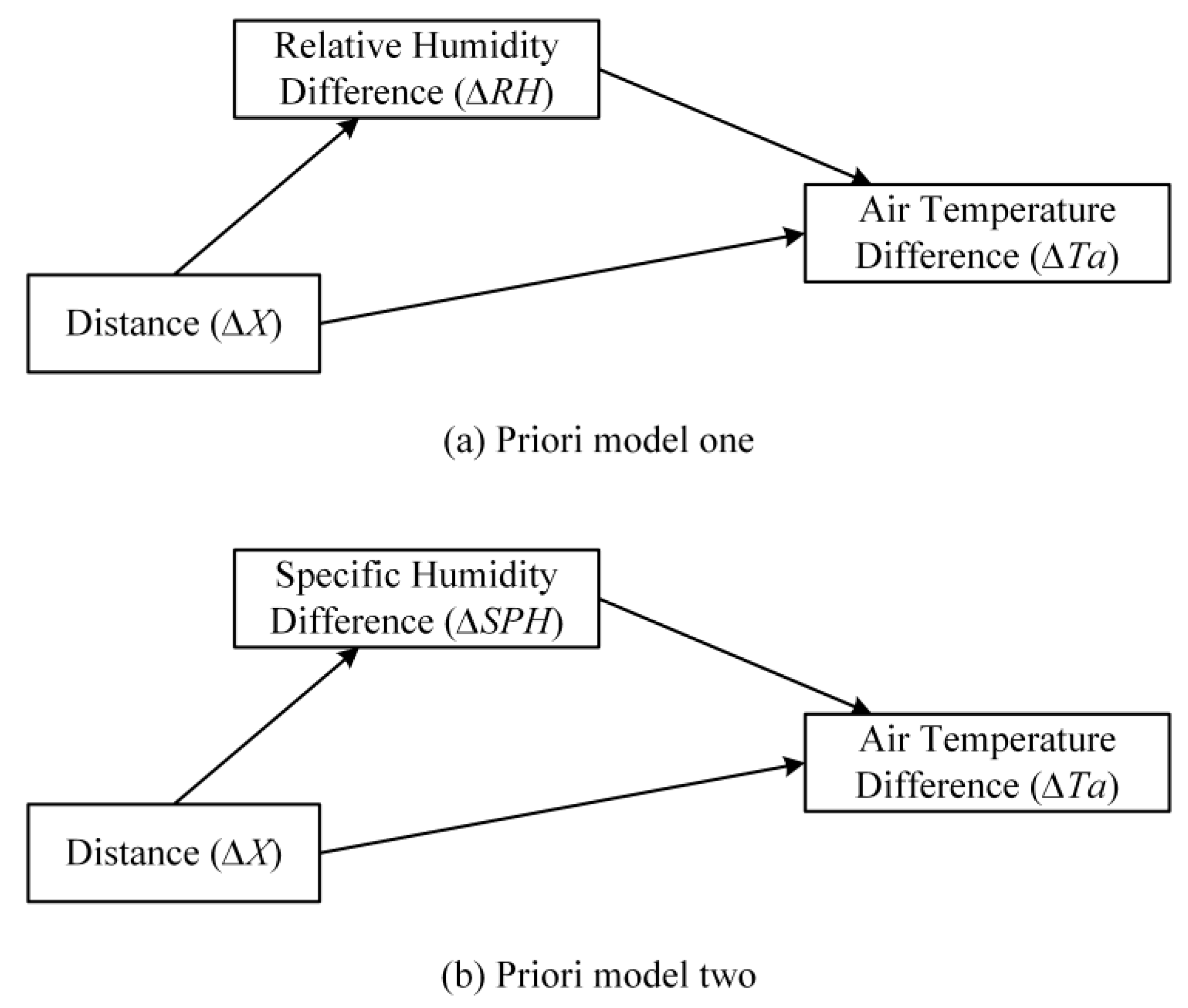
Path analysis was used to explore the causality of air temperature variation in the study site. In a path analysis model, the path coefficients describe the strength of causal relationships between variables; the standardized forms of the path coefficients, also called standardized regression weights, are directly analogous to partial correlation coefficients. With the paths, the method can evaluate direct and indirect causal effects of one variable on another [41]. Two priori models representing the relationships between variables are considered in our study, which are illustrated in Figure 2. We hypothesize that increases in ∆X would decrease ∆RH and ∆SPH, and would increase ∆Ta, and that increases in ∆RH or ∆SPH would decrease ∆Ta. The direct link path between two variables represents the direct effect between them, while the path between two variables mediated by other variables represents the indirect effect. We then conducted the path analysis based on maximum likelihood (ML) estimation in R by using the lavaan package [42]. The path analysis models were estimated by using t-statistics tests to evaluate the significance of the individual path coefficients. Additionally, the R-squared value was also calculated to reflect the proportion of variance in the response variable that can be accounted for by the explanatory variables.

2.4. Genetic Support Vector Regression

In this study, the genetic support vector regression, a combination of genetic algorithm and support vector regression (SVR), was used to fit the relationship of Air Temperature Difference (∆Ta) with Distance (∆X) and humidity difference (∆RH or ∆SPH). The framework of the method is illustrated in Figure 3. Whether to use variable ∆RH or ∆SPH for input depends on the results of the path analysis. The traditional support vector regression requires some parameters to be set with priority, and the values of these parameters affect the precision of the regression model. Thus, finding the proper values of these parameters is crucial for SVR. Since the genetic algorithm is good at searching for the globally optimal solution of a problem, we introduced it to SVR training to find the optimal values of the parameters. Then, we used the optimal values to obtain the SVR model that represent the approximate relationship of ∆X and humidity difference (∆RH or ∆SPH) to ∆Ta. Thereafter, we use the obtained SVR model to simulate the independent contributions of ∆X and humidity difference (∆RH or ∆SPH) to ∆Ta. The short description of the SVR is presented in Section 2.4.1, and the description of using the genetic algorithm to find the optimal parameters values for SVR is presented in Section 2.4.2. The SVR process was implemented by employing the LIBSVM package [43], which is a library for support vector machines.

2.4.1. Support Vector Regression

Support vector regression (SVR) is a statistical technique to fit regression models by using support vector machine (SVM), which is a supervised learning method based on statistical learning theory and is also widely used in classification. Through introducing kernel function, SVR has a remarkable advantage in dealing with nonlinear problems. Given a training sample S = {(x1, y1), …, (xn, yn)}, the regression function that approximates the true relationship between yi and xi in SVR is specified in the following form:
y = f ( x ) = w T φ ( x ) + b
where φ represents the nonlinear mapping function transforming x into a higher dimensional feature space; w is a weight vector of which the dimension is same as the feature space of φ; b is the bias. In the situation of this study, x represents a vector that consists of ∆X and humidity difference (∆RH or ∆SPH), and y represents ∆Ta. To evaluate the fitting error of the model, a loss function was used in SVR. The most commonly used loss function is the ε insensitive, which is defined as
V ( x , y , f ) = | y f ( x ) | ε = max { 0 , | y f ( x ) | ε }
A desirable solution of regression requires the model both to be flat and have a small fitting error. Flatness means that the norm of the weight coefficient vector w, representing the length in the high dimensional feature space, should be small; the small fitting error emphasizes that the sum of the loss function should be minimum. Then, the problem can be written as an optimization:
min   1 2 w 2 + C i = 1 n V ( x i , y i , f ) ,
where C is a constant (C > 0) controlling the trade-off between the flatness and the tolerable fitting error. By using Lagrangian transformation and applying the Karush–Kuhn–Tucker (KKT) complementary conditions, we acquire the dual form of the optimization problem, which is described as
max   1 2 i , j = 1 n ( α i α i * ) ( α j α j * ) φ ( x i ) , φ ( x j ) ε i = 1 n ( α i + α i * ) + i = 1 n y i ( α i α i * ) ,
subject to:
i = 1 n ( α i α i * ) = 0 ,
0 α i , α i * C , i = 1 , , n ,
where αi and αi* are Lagrange multipliers, and ⟨φ(xi), φ(xj)⟩ donates the inner product of φ(xi) and φ(xj). Since Equation (7) is a quadratic function depending only on αi and αi*, it can be solved by Sequential Minimal Optimization (SMO) algorithm or Quadratic Programming (QP) techniques. Furthermore, using the so-called kernel function expressed as an inner product, k(xi, xj) = ⟨φ(xi), φ(xj)⟩, the regression function of Equation (4) can be given as
f ( x ) = i = 1 n ( α i α i * ) k ( x i , x ) + b .
Four types of kernel functions are commonly used in SVR models; these are linear, polynomial, radial basis function, and sigmoid. In this study, we adopted the sigmoid kernel, for it performs similarly to the radial basis function for certain parameters [44] but may be better than radial basis functions in global trends. The sigmoid kernel is defined as:
k ( x , x ) = tanh ( γ x T x + r ) , γ > 0 ,
where γ is the regularization coefficient and r is the bias term.

2.4.2. Genetic Algorithm to Optimize SVR Parameters

In SVR training, the values of parameters C, ε, γ and r, respectively, in Equations (6), (7) and (11), must be given with priority, and these values would affect the precision of the regression model. To find the optimum values, Genetic algorithm (GA) and a five-fold cross-validation were employed in this study. The derivative-free optimization strategy, as a type of population-based evolutionary algorithm, allows GA to always yield a global optimum solution. We used the mean square error (MSE) between predicted values and observed values to measure the prediction accuracy of the regression model. The MSE is defined as
M S E = 1 n i = 1 n ( y ^ i y i ) 2 ,
where ŷi is the predicted value of the regression model with respect to xi; yi is the ith observed value of y in the training sample. In addition, the coefficient of determination was calculated to indicate the prediction accuracy of the model in this study, which is given as
R 2 = 1 i = 1 n ( y ^ i y i ) 2 / i = 1 n ( y i y ¯ ) 2 = 1 n · M S E / i = 1 n ( y i y ¯ ) 2 .
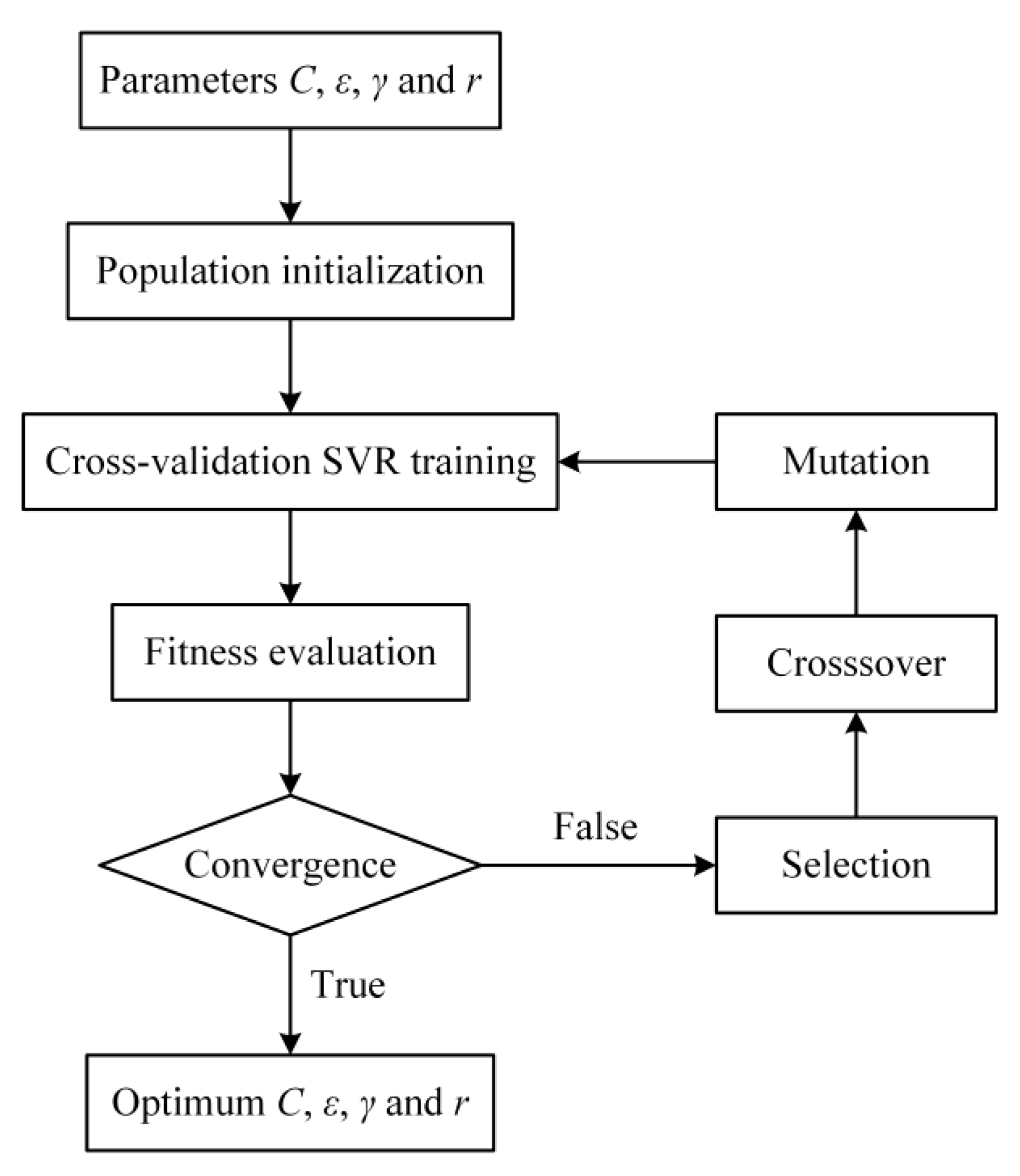
The overall procedure of a genetic algorithm for finding optimum values of C, ε, γ and r is shown in Figure 4. The algorithm begins with the random initialization of a population, in which each chromosome denotes a set values of C, ε, γ and r that use a real-number representation. Then SVR training with five-fold cross-validation was performed, and the fitness values of the population were calculated. The fitness function is as follows:
F = 1 / M S E .
The GA operators, which consist of selection, crossover, and mutation, as well as SVR training were repeatedly conducted. Additionally, the fitness values of the population were repeatedly evaluated until the fitness function becomes steady in the sense that its value of the best population does not change for several generations. In this case, GA is said to be converged. The best population provided by GA convergence will be close to the global minimum of the MSE, thus obtaining the optimum values of C, ε, γ and r. Then, we introduced these optimum values to SVR training, and used the whole measured data for it, without cross-validation. Thereafter, we obtained the SVR model that represents the relationship of ∆X and humidity difference (∆RH or ∆SPH) to ∆Ta, in the form of Equation (10).
After establishing the SVR model, we used it to simulate the ∆Ta with ∆X and humidity difference (∆RH or ∆SPH). In detail, we ran the SVR model by varying the value of one input and fixing the value of another input to obtain the output value, and then evaluated the range of the variation of the output to explore the relationship of the output with the varied input, thereafter quantifying the independent contributions of ∆X and humidity difference (∆RH or ∆SPH) to ∆Ta.

3. Results and Discussion

3.1. Distributions of ∆Ta and ∆RH of the Two Land Covers

Through field measurements, a dataset with a sample size of 130 was obtained. Figure 5 displays the box plots of the Air Temperature Difference (∆Ta) and the Relative Humidity Difference (∆RH) of the bush woodland and the concrete land. It can be seen that the ∆Ta is obviously different between these two land covers, as is the ∆RH. Furthermore, the ∆Ta of the concrete land is generally larger than 0, which indicates that the air temperatures of the concrete land are generally higher than those of the reference point. When considering the bush woodland, the ∆Ta is generally less than 0, indicating the air temperatures generally lower than those of reference point. As to the relative humidity, the values of the bush woodland are generally higher, and the values of the concrete land are generally lower than those of the reference point.
Additionally, Kruskal–Wallis one-way analysis of variance (ANOVA) was performed to further validate whether the ∆Ta and the ∆RH distributions significantly vary by land covers. The results are shown in Table 1 and suggest that the distributions of ∆Ta and ∆RH are significantly distinguished between the two land covers (p < 0.001).

3.2. Effects of Variables on ∆Ta in Priori Models

We conducted the path analyses of the two priori models illustrated in Figure 2, respectively. The path analysis results of priori model one are shown in Table 2. As can be seen, ∆X and ∆RH explain 87% variation of the ∆Ta, and ∆X and ∆RH have direct effects of 0.143 and −0.822, respectively. The fact that the effect of ∆X is positive indicates that the farther away from the reference point toward concrete land, the higher the air temperature, and the farther toward bush woodland, the lower the air temperature. This suggests that the land cover has a direct effect on air temperature; that is, the concrete land has higher air temperature than the bush woodland. As to ∆RH, the negative effect indicates that an increase in relative humidity is to cause a decrease in air temperature.
Moreover, the absolute value of the direct effect of ∆RH is much larger than that of ∆X. However, 54.7% variation of the ∆RH can be explained by the ∆X, and the direct effect of ∆X on ∆RH is −0.740. Then, we can obtain that the indirect effect of ∆X on ∆Ta is 0.608 = (−0.822) × (−0.740), and the total effect of the ∆X on ∆Ta is 0.751 = 0.143 + 0.608, which is very large and only a little less than the absolute value of the effect of ∆RH. This explains why the land cover significantly affects the variation of the local air temperature, but the results also indicate that most of this effect is indirect and mediated through the ∆RH, which implies that we can modify the effect through the mediated factor without land cover change.
The path analysis results of priori model two are shown in Table 3. As to this model, the t-statistics test results of the path coefficients are also significant. However, ∆X and ∆SPH only explain 57.4% of the variation of the ∆Ta. Additionally, ∆X can only explain 15% variation of the ∆SPH, while ∆X explains 54.7% of the ∆RH in priori model one. The results suggest that there would be additional factors combined to explain the variation of the ∆SPH. For example, the area with higher saturation specific humidity may be more likely to have higher specific humidity. As to ∆Ta, the latent heat flux accounts for part of its variation in physical perspective. Meanwhile, the latent heat flux is directly proportional to the vertical specific humidity gradient. This gradient may perhaps also be affected by saturation specific humidity. Perhaps even the same specific humidity near the land surface in the condition with higher saturation specific humidity may present a smaller specific humidity gradient in the vertical direction compared with in the condition with lower saturation specific humidity, for the upper specific humidity might be higher in the former condition than in the latter condition. Thus, ∆SPH may be not enough to explain the variations of the ∆Ta affected by latent heat flux. The results of path analysis with respect to priori model two also indicate that the absolute value of the effect of ∆SPH on ∆Ta is very small, although the effect is negative.
For the end of this section, we want to further clarify the terminologies of “direct effect” and “indirect effect” in this study to avoid possible misunderstandings. The two terminologies, which are defined in Section 2.3, are just based on the priori path analysis model. Their meanings may not exactly correspond with the physical processes but are just convenient to reflect the links between the factors considered in the study. In physics, we note that sometimes it is difficult to distinguish between direct and indirect effects, for almost any physical process can be broken down into many subprocesses. For this study, to identify the direct and the indirect effects of land cover on air temperature in physics, as seen from the models in Figure 2, it can be argued that the direct effect is the impact from the processes including net radiation absorption, sensible heat conduction, etc., but excluding the evapotranspiration. In contrast, the indirect effect is the impact from the evapotranspiration process. The corresponding physical meanings may be changed when considering other priori models.

3.3. Independent Contributions of ∆X and ∆RH

Since ∆X and ∆RH explain more variation of the ∆Ta than ∆X and ∆SPH according to path analysis, we used genetic SVR to fit the relationship of ∆Ta with ∆X and ∆RH. We carried out the SVR training combined with GA to find the optimum values of C, ε, γ, and r, which are, respectively, 85.214, 0.1250, 0.6153, and −1.3775. The MSE of the five-fold cross-validation was 0.4378, and the corresponding coefficient of determination was 0.878. Then, we set the parameters C, ε, γ, and r to the optimum values, and used the whole measured data for SVR training without cross-validation. This time, the MSE was 0.3703 and the coefficient of determination was 0.897. These results indicate that the SVR model is with good fitness. Thereafter, we used the SVR model to simulate independent contributions of ∆X and ∆RH to ∆Ta.
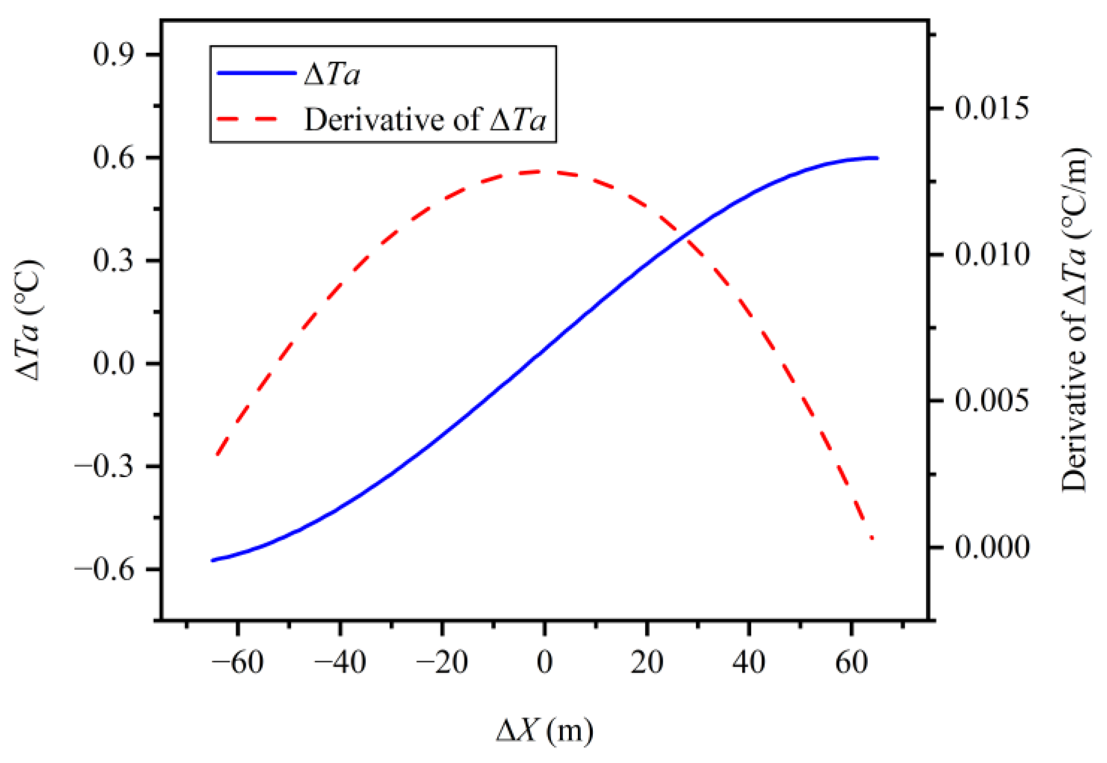
First, we varied the ∆X from −65 to 65 m, keeping the ∆RH at 0, and then used the SVR model to calculate ∆Ta. The simulation results are shown in Figure 6. It can be seen that at the concrete land (∆X > 0), the ∆Ta is positive and increases as the ∆X increases. When at the bush woodland, the ∆Ta is negative, and its absolute value also increases as the absolute value of ∆X increases.
We also analyzed the derivative of ∆Ta to ∆X. The derivative reached a peak of 0.013 °C/m at the ∆X of around 0 (Figure 6). When only considering the effect of the land cover, it means that the change rate of the air temperature is at its maximum at the boundary between the two land plots, and that the increase rate at the concrete land and the decrease rate at the bush woodland both become slower as the distances from the boundary increase.
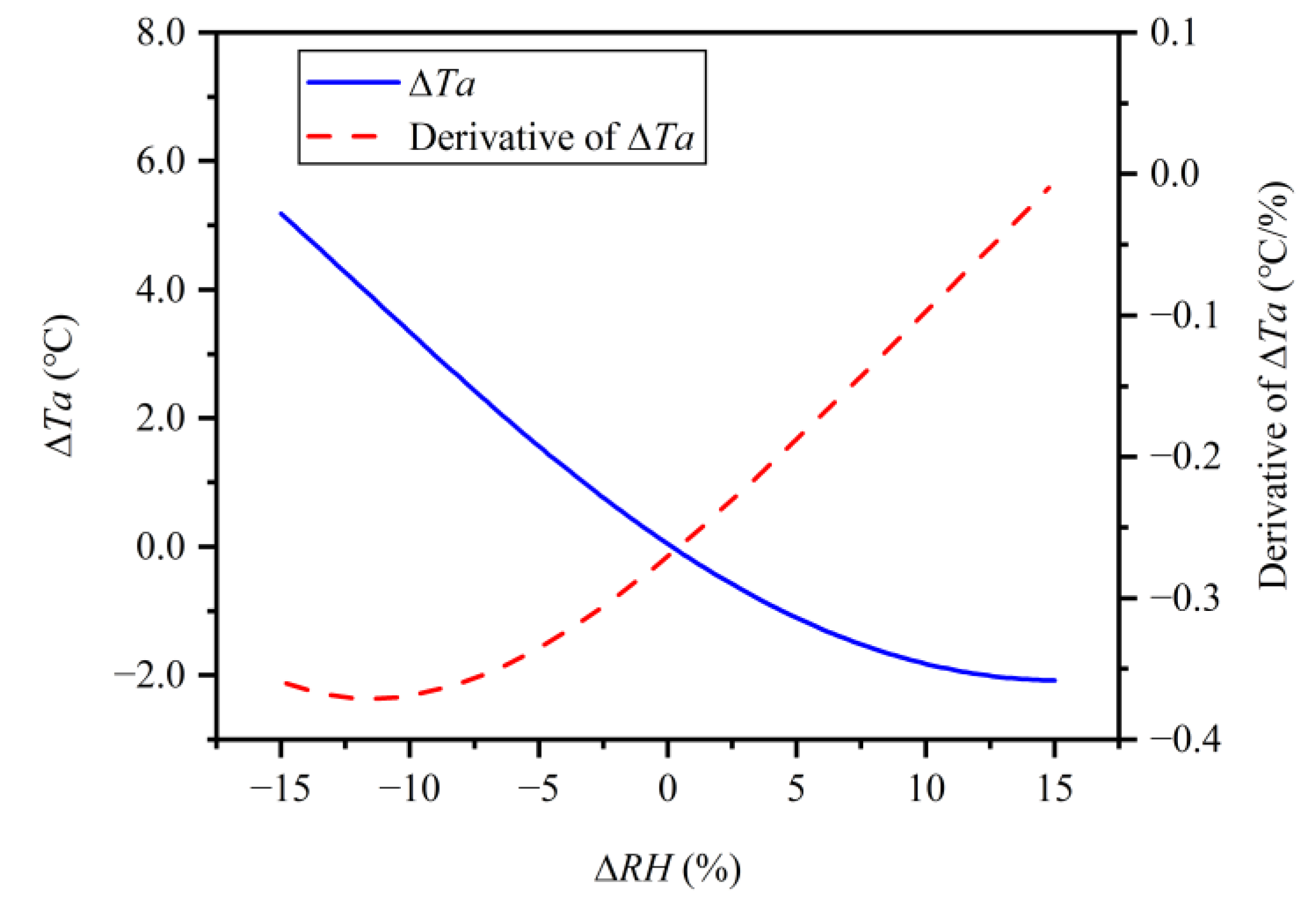
Second, we maintained the ∆X at 0 and varied the ∆RH from −15% to 15%, calculating the ∆Ta by using the SVR model. As seen from Figure 7, the ∆RH has considerable influence on the ∆Ta. When the relative humidity is 15% less than the reference point, the air temperature could be about 5 °C higher than the reference point; when the relative humidity is 15% larger, the air temperature could be about 2 °C lower. In contrast, as ∆X varies from −65 to 65 m, the absolute values of the ∆Ta are not more than 0.6 °C (Figure 6).
Additionally, Figure 7 shows the derivative of the ∆Ta to the ∆RH. As can be seen, the absolute value of the derivative is maximum at the ∆RH of about −11.5%, not at the ∆RH of 0. This is because the temperature decrease rate is influenced by the context of the relative humidity. In this study, the average value of the relative humidity with respect to the reference point is 47.1%. Thus, the influence of increasing relative humidity on decreasing air temperature might be largest when the relative humidity is 35.6%. In this situation, relative humidity increasing by 1% would lead to air temperature decreasing by approximately 0.37 °C (Figure 7).
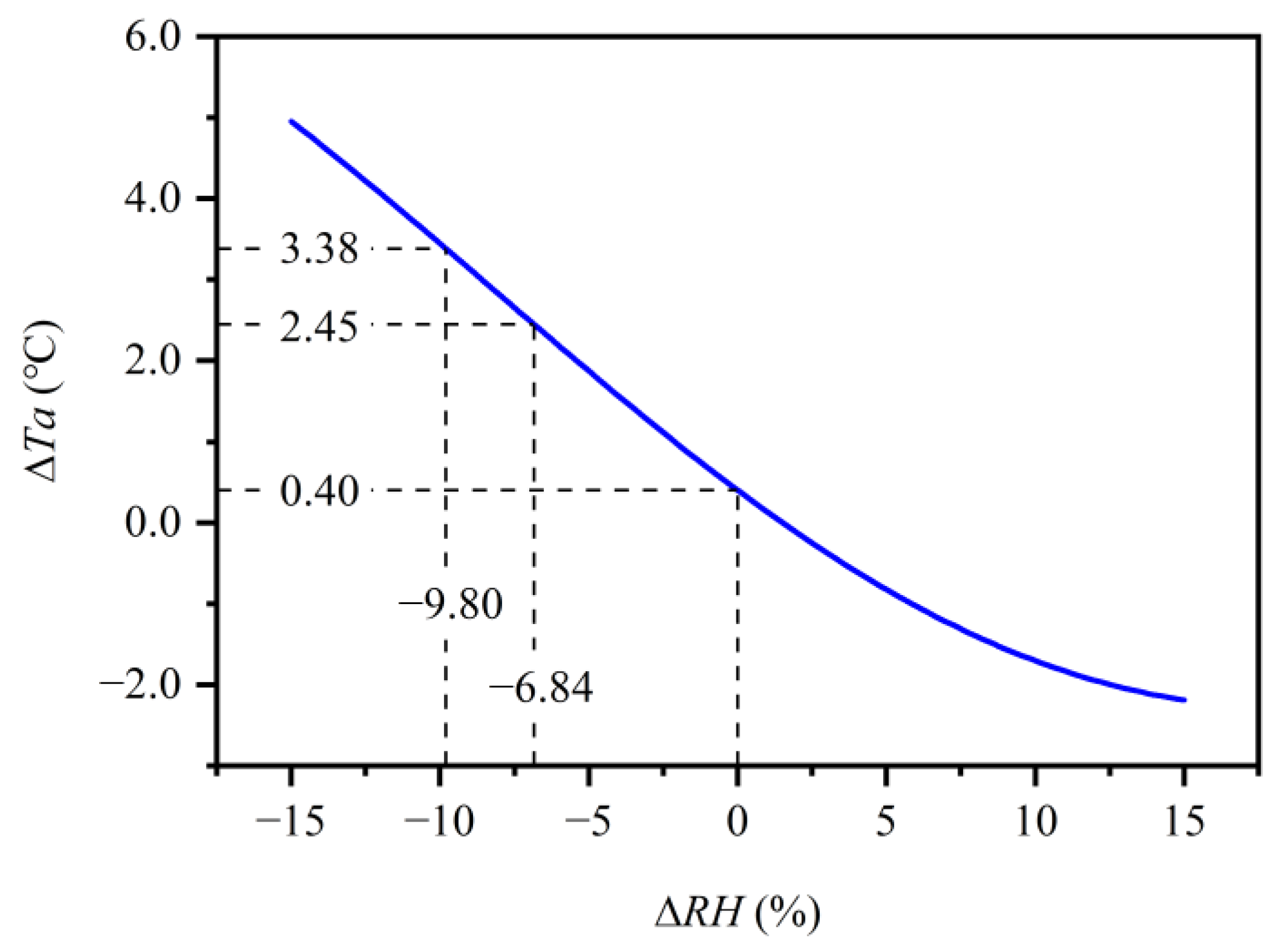
Furthermore, considering the concrete land, the average value of the ∆Ta in observations is 2.42 °C, and the 75% quantile value of the ∆Ta in observations is 3.43 °C (Figure 5a). Since the contribution of the ∆X is less than 0.6 °C (Figure 6), the contributions of the ∆RH are nearly 1.82 and 2.83 °C. We further simulated the ∆Ta with the ∆X of 30 m, near the center of the concrete land, by varying the ∆RH. The simulation results are shown in Figure 8. Meanwhile, the average and the 25% quantile observed values of the ∆RH at the concrete land are −6.84% and −9.80%, respectively (Figure 5b). According to the simulation results, the values of ∆Ta corresponding to these two values of the ∆RH are, respectively, 2.45 and 3.38 °C (Figure 8), which are almost consistent with the average and the 75% quantile values of observed ∆Ta (2.42 and 3.43 °C mentioned above). Now, it could be safe to conclude that the contribution of the land cover is about 0.40 °C (at the point of ∆RH = 0 in Figure 8) and the contributions of the relative humidity differences are about 2.05 and 2.98 °C. By only considering the point at ∆RH of −6.84%, which is the average ∆RH of the concrete land, the percentage contribution of the land cover and the relative humidity difference could be obtained with 16.3% = 0.40/2.45 and 83.7% = 2.05/2.45, which could be considered as the average contribution levels of these two factors to the rise of the air temperature at the concrete land in the study site.

3.4. Implication for High Air Temperature Mitigation

To mitigate high air temperatures and heat waves in a city, increasing green land is an often-proposed strategy. However, when in the built-up area, this strategy might be difficult to apply. The results of this study would shed light on the mitigation of high air temperatures in this situation. Although the concrete land appears with higher air temperature than the vegetated land, path analysis results show that, actually, the direct effect of ∆X on ∆Ta is small, while its indirect effect mediated through ∆RH is larger than four times the value of the direct effect. Moreover, the direct effect of ∆RH is nearly six times that of ∆X, even larger than the total effect of the ∆X. The simulation results by using the SVR model also show that the independent contribution of the ∆X is not more than one-fifth that of the ∆RH.
The study results suggest that the relative humidity difference plays a key role in air temperature difference. If a land cover experiences no change, it might be impossible to offset its direct effect on air temperature difference. However, it is possible to modify the indirect effect by controlling the linkages. The fact that the indirect effect of the land cover is much larger than the direct effect is also benefit for decreasing the total effect on air temperature difference by regulating the mediated factor, relative humidity difference.
Therefore, an alternative strategy to reduce the local high air temperature of the city, especially in the built-up area, is to increase the humidity artificially. In fact, an increase in relative humidity by 5–10% might obtain a good effect. As can be seen from Figure 8, the 10% lower relative humidity could lead to a 3.0 °C higher air temperature, and 5% lower relative humidity could lead to a 1.5 °C higher temperature, compared with the reference point. Thus, we can assume that if we compensate the relative humidity with a 5–10% increase in the concrete land of the study site, the air temperature might decrease 1.5–3.0 °C.
In fact, the measures associated with the strategy of increasing humidity to reduce ambient air temperature have been known for centuries, and have recently been developing and are being tested around the world. Santamouris et al. [45] reviewed the systems with respect to these measures such as pools, ponds, water sprinklers, and fountains, and found that water spraying was the most effective at cooling air temperature. The case studies of theoretical calculations in Beirut, Lebanon, and experiments in Seville, Spain, displayed that the average temperatures of the ambient air decreased between 3 and 4 °C by using water spray systems. Additionally, in Japan, where most of the cities have humid subtropical climates, use of water mist spraying is increasing popular to cool urban spaces and yields temperature reductions about 2–3 °C on hot summer days [46,47]. These studies support our discussion above to some extent, and indicate that increasing the humidity artificially, such as by water spraying, is a workable solution for mitigating high urban air temperatures in many cities. As to our study, the path analysis and the SVR simulation results illustrate that increasing humidity could be an effective strategy available to cool air temperature compared with expanding vegetation.
Furthermore, spray cooling is easily integrated in existing city infrastructures and is extremely versatile, with high local impacts in a cost-effective and controllable way [47]. The technology can be implemented on pavements and squares without vegetation. Of course, the application of this technology depends on the climatic context. Previous studies suggested that the water mist system should be stopped when the relative humidity is over 70% [33,48,49].

4. Conclusions

Given the adverse influences posed by high air temperatures and heat waves and in the light of the views that land cover changes impact on local climate, this study performed the field measurements of air temperature and relative humidity. Thereafter, the study used path analysis to examine the direct and indirect effects of land cover and humidity differences on air temperature differences, and employed an SVR simulation to quantify the independent contributions of the two factors to it. The test results of the path analysis indicate that land cover and relative humidity difference can explain most variation of the air temperature difference, and that the path coefficients are very significant. Additionally, the training results of the SVR model, combined with genetic algorithm, show that the SVR model could fit the air temperature difference very well.
The path analysis illustrates that the total effect of land cover on air temperature difference is large. However, most of the effect is indirect and mediated through relative humidity difference, with a small direct effect on air temperature difference. In contrast, the direct effect of relative humidity difference on air temperature difference is very large, even a little larger than the total effect of land cover. Moreover, the SVR simulation further reveals that the relative humidity difference could contribute much more to air temperature difference compared with land cover. These results suggest that relative humidity differences significantly affect air temperature differences. The higher air temperature on land cover without vegetation might be mostly due to the lower humidity compared with vegetated land cover.
Even though expanding vegetation is often recommended by many studies, the results of this study imply that increasing humidity artificially could be an alternative strategy to reduce the local high air temperature of the city. This strategy might be especially useful and effective in built-up areas. Our study identifies the effect of relative humidity difference and quantifies its contribution to air temperature differences in the study site, and thereby would provide additional scientific support for the effectiveness of the strategy relevant to increasing humidity.
One limitation of this study is that there is a need to further illustrate the physical mechanism of the effect of relative humidity difference on air temperature difference. Thus, the effect of relative humidity difference on the specific humidity gradient in the vertical direction should be addressed. The study has illustrated that the effect of specific humidity differences on air temperature differences is small. Therefore, only considering the specific humidity variation would be not enough. Instead, the variation of the vertical specific humidity gradient must be focused on in future. Another limitation of the study is that the effects of wind speed and wind direction are not considered, although the wind speed of the study site is small. Since the wind speed and the wind direction often change, their effects on air temperature variation are complex. To address this problem, it is required to redesign the study. We will focus on the above limitations in future work. Regardless of the limitations, however, the studies are encouraging.

Author Contributions

Designed the research, W.S., N.W. and A.X.; performed the field measurements, N.W., A.X. and L.L.; analyzed the data and wrote the article, W.S.; discussed the results, J.H. and Y.Z. All authors have read and agreed to the published version of the manuscript.

Funding

This research was funded by National Natural Science Foundation of China (NSFC), grant number 41701179.

Conflicts of Interest

The authors declare no conflict of interest.

References

  1. Crutzen, P.J. New Directions: The growing urban heat and pollution “island” effect–Impact on chemistry and climate. Atmos. Environ. 2004, 38, 3539–3540. [Google Scholar] [CrossRef]
  2. Jacob, D.J.; Winner, D.A. Effect of climate change on air quality. Atmos. Environ. 2009, 43, 51–63. [Google Scholar] [CrossRef] [Green Version]
  3. Anderson, B.G.; Bell, M.L. Weather-Related Mortality How Heat, Cold, and Heat Waves Affect Mortality in the United States. Epidemiology 2009, 20, 205–213. [Google Scholar] [CrossRef] [Green Version]
  4. D’Ippoliti, D.; Michelozzi, P.; Marino, C.; de’Donato, F.; Menne, B.; Katsouyanni, K.; Kirchmayer, U.; Analitis, A.; Medina-Ramon, M.; Paldy, A.; et al. The impact of heat waves on mortality in 9 European cities: Results from the EuroHEAT project. Environ. Health 2010, 9, 37. [Google Scholar] [CrossRef] [PubMed] [Green Version]
  5. Yu, W.W.; Mengersen, K.; Wang, X.Y.; Ye, X.F.; Guo, Y.M.; Pan, X.C.; Tong, S.L. Daily average temperature and mortality among the elderly: A meta-analysis and systematic review of epidemiological evidence. Int. J. Biometeorol. 2012, 56, 569–581. [Google Scholar] [CrossRef] [PubMed] [Green Version]
  6. Yang, J.; Liu, H.Z.; Ou, C.Q.; Lin, G.Z.; Ding, Y.; Zhou, Q.; Shen, J.C.; Chen, P.Y. Impact of Heat Wave in 2005 on Mortality in Guangzhou, China. Biomed. Environ. Sci. 2013, 26, 647–654. [Google Scholar]
  7. Mazdiyasni, O.; AghaKouchak, A.; Davis, S.J.; Madadgar, S.; Mehran, A.; Ragno, E.; Sadegh, M.; Sengupta, A.; Ghosh, S.; Dhanya, C.T.; et al. Increasing probability of mortality during Indian heat waves. Sci. Adv. 2017, 3, e1700066. [Google Scholar] [CrossRef] [Green Version]
  8. Fritze, T. The Effect of Heat and Cold Waves on the Mortality of Persons with Dementia in Germany. Sustainability 2020, 12, 13. [Google Scholar] [CrossRef]
  9. Kang, C.; Park, C.; Lee, W.; Pehlivan, N.; Choi, M.; Jang, J.; Kim, H. Heatwave-Related Mortality Risk and the Risk-Based Definition of Heat Wave in South Korea: A Nationwide Time-Series Study for 2011–2017. Int. J. Env. Res. Public Health 2020, 17, 12. [Google Scholar] [CrossRef] [PubMed]
  10. Schlegel, I.; Muthers, S.; Mucke, H.G.; Matzarakis, A. Comparison of Respiratory and Ischemic Heart Mortalities and their Relationship to the Thermal Environment. Atmosphere 2020, 11, 18. [Google Scholar] [CrossRef]
  11. Oerlemans, J. Quantifying global warming from the retreat of glaciers. Science 1994, 264, 243–245. [Google Scholar] [CrossRef] [PubMed] [Green Version]
  12. Karl, T.R.; Trenberth, K.E. Modern global climate change. Science 2003, 302, 1719–1723. [Google Scholar] [CrossRef] [PubMed] [Green Version]
  13. Meehl, G.A.; Tebaldi, C. More intense, more frequent, and longer lasting heat waves in the 21st century. Science 2004, 305, 994–997. [Google Scholar] [CrossRef] [PubMed] [Green Version]
  14. Perkins, S.E.; Alexander, L.V.; Nairn, J.R. Increasing frequency, intensity and duration of observed global heatwaves and warm spells. Geophys. Res. Lett. 2012, 39, 5. [Google Scholar] [CrossRef]
  15. Serrano, J.P.; Diaz, F.J.A.; Garcia, J.A.G. Analysis of Extreme Temperature Events over the Iberian Peninsula during the 21st Century Using Dynamic Climate Projections Chosen Using Max-Stable Processes. Atmosphere 2020, 11, 26. [Google Scholar]
  16. Zhao, W.; Zhou, N.F.; Chen, S.F. The Record-Breaking High Temperature over Europe in June of 2019. Atmosphere 2020, 11, 12. [Google Scholar] [CrossRef]
  17. Razzaghmanesh, M.; Beecham, S.; Brien, C.J. Developing resilient green roofs in a dry climate. Sci. Total Environ. 2014, 490, 579–589. [Google Scholar] [CrossRef]
  18. Hansen, J.; Sato, M.; Ruedy, R.; Lacis, A.; Oinas, V. Global warming in the twenty-first century: An alternative scenario. Proc. Natl. Acad. Sci. USA 2000, 97, 9875–9880. [Google Scholar] [CrossRef] [Green Version]
  19. Duan, A.M.; Wu, G.X.; Zhang, Q.; Liu, Y.M. New proofs of the recent climate warming over the Tibetan Plateau as a result of the increasing greenhouse gases emissions. Chin. Sci. Bull. 2006, 51, 1396–1400. [Google Scholar] [CrossRef]
  20. Kalnay, E.; Cai, M. Impact of urbanization and land-use change on climate. Nature 2003, 423, 528–531. [Google Scholar] [CrossRef]
  21. He, J.J.; Yu, Y.; Yu, L.J.; Yin, C.M.; Liu, N.; Zhao, S.P.; Chen, X. Effect of soil texture and hydraulic parameters on WRF simulations in summer in east China. Atmos. Sci. Lett. 2016, 17, 538–547. [Google Scholar] [CrossRef] [Green Version]
  22. Arnfield, A.J. Two decades of urban climate research: A review of turbulence, exchanges of energy and water, and the urban heat island. Int. J. Climatol. 2003, 23, 1–26. [Google Scholar] [CrossRef]
  23. Arribas, A.; Gallardo, C.; Gaertner, M.A.; Castro, M. Sensitivity of the Iberian Peninsula climate to a land degradation. Clim. Dyn. 2003, 20, 477–489. [Google Scholar] [CrossRef]
  24. Masson, V. Urban surface modeling and the meso-scale impact of cities. Theor. Appl. Climatol. 2006, 84, 35–45. [Google Scholar] [CrossRef]
  25. Pielke, R.A. Land use and climate change. Science 2005, 310, 1625–1626. [Google Scholar] [CrossRef] [Green Version]
  26. Dirmeyer, P.A.; Niyogi, D.; de Noblet-Ducoudre, N.; Dickinson, R.E.; Snyder, P.K. Impacts of land use change on climate. Int. J. Climatol. 2010, 30, 1905–1907. [Google Scholar] [CrossRef] [Green Version]
  27. Luck, G.W.; Smallbone, L.T.; O’Brien, R. Socio-Economics and Vegetation Change in Urban Ecosystems: Patterns in Space and Time. Ecosystems 2009, 12, 604–620. [Google Scholar] [CrossRef]
  28. Bowler, D.E.; Buyung-Ali, L.; Knight, T.M.; Pullin, A.S. Urban greening to cool towns and cities: A systematic review of the empirical evidence. Landsc. Urban Plann. 2010, 97, 147–155. [Google Scholar] [CrossRef]
  29. Deilami, K.; Kamruzzaman, M.; Liu, Y. Urban heat island effect: A systematic review of spatio-temporal factors, data, methods, and mitigation measures. Int. J. Appl. Earth Obs. Geoinf. 2018, 67, 30–42. [Google Scholar] [CrossRef]
  30. Amani-Beni, M.; Zhang, B.; Xie, G.D.; Xu, J. Impact of urban park’s tree, grass and waterbody on microclimate in hot summer days: A case study of Olympic Park in Beijing, China. Urban For. Urban Green. 2018, 32, 1–6. [Google Scholar] [CrossRef]
  31. Meili, N.; Manoli, G.; Burlando, P.; Bou-Zeid, E.; Chow, W.T.L.; Coutts, A.M.; Daly, E.; Nice, K.A.; Roth, M.; Tapper, N.J.; et al. An urban ecohydrological model to quantify the effect of vegetation on urban climate and hydrology (UT&C v1.0). Geosci. Model Dev. 2020, 13, 335–362. [Google Scholar]
  32. Myrup, L.O. A Numerical Model of the Urban Heat Island. J. Appl. Meteorol. 1969, 8, 908–918. [Google Scholar] [CrossRef]
  33. Ulpiani, G.; Di Giuseppe, E.; Di Perna, C.; D’Orazio, M.; Zinzi, M. Thermal comfort improvement in urban spaces with water spray systems: Field measurements and survey. Build. Environ. 2019, 156, 46–61. [Google Scholar] [CrossRef]
  34. Montazeri, H.; Toparlar, Y.; Blocken, B.; Hensen, J.L.M. Simulating the cooling effects of water spray systems in urban landscapes: A computational fluid dynamics study in Rotterdam, The Netherlands. Landsc. Urban Plann. 2017, 159, 85–100. [Google Scholar] [CrossRef]
  35. Xue, F.; Li, X.F.; Ma, J.; Zhang, Z.Q. Modeling the influence of fountain on urban microclimate. Build. Simul. 2015, 8, 285–295. [Google Scholar] [CrossRef]
  36. Fahed, J.; Kinab, E.; Ginestet, S.; Adolphe, L. Impact of urban heat island mitigation measures on microclimate and pedestrian comfort in a dense urban district of Lebanon. Sust. Cities Soc. 2020, 61, 14. [Google Scholar]
  37. Ulpiani, G. Water mist spray for outdoor cooling: A systematic review of technologies, methods and impacts. Appl. Energy 2019, 254, 30. [Google Scholar] [CrossRef]
  38. Hu, Y.H.; Hou, M.T.; Jia, G.S.; Zhao, C.L.; Zhen, X.J.; Xu, Y.H. Comparison of surface and canopy urban heat islands within megacities of eastern China. ISPRS-J. Photogramm. Remote Sens. 2019, 156, 160–168. [Google Scholar] [CrossRef]
  39. Peng, S.J.; Feng, Z.L.; Liao, H.X.; Huang, B.; Peng, S.L.; Zhou, T. Spatial-temporal pattern of, and driving forces for, urban heat island in China. Ecol. Indic. 2019, 96, 127–132. [Google Scholar] [CrossRef]
  40. Murray, F.W. On the Computation of Saturation Vapor Pressure. J. Appl. Meteorol. 1967, 6, 203–204. [Google Scholar] [CrossRef]
  41. Tomarken, A.J.; Waller, N.G. Structural equation modeling: Strengths, limitations, and misconceptions. Ann. Rev. Clin. Psych. 2005, 1, 31–65. [Google Scholar] [CrossRef] [PubMed] [Green Version]
  42. Rosseel, Y. lavaan: An R Package for Structural Equation Modeling. J. Stat. Softw. 2012, 48, 1–36. [Google Scholar] [CrossRef] [Green Version]
  43. Chang, C.C.; Lin, C.J. LIBSVM: A Library for Support Vector Machines. ACM Trans. Intell. Syst. Technol. 2011, 2, 27. [Google Scholar] [CrossRef]
  44. Song, S.T.; Zhan, Z.C.; Long, Z.Y.; Zhang, J.C.; Yao, L. Comparative Study of SVM Methods Combined with Voxel Selection for Object Category Classification on fMRI Data. PLoS ONE 2011, 6. [Google Scholar] [CrossRef]
  45. Santamouris, M.; Ding, L.; Fiorito, F.; Oldfield, P.; Osmond, P.; Paolini, R.; Prasad, D.; Synnefa, A. Passive and active cooling for the outdoor built environment–Analysis and assessment of the cooling potential of mitigation technologies using performance data from 220 large scale projects. Sol. Energy 2017, 154, 14–33. [Google Scholar] [CrossRef]
  46. Farnham, C.; Nakao, M.; Nishioka, M.; Nabeshima, M.; Mizuno, T. Study of mist-cooling for semi-enclosed spaces in Osaka, Japan. Procedia Environ. Sci. 2011, 4, 228–238. [Google Scholar] [CrossRef] [Green Version]
  47. Farnham, C.; Emura, K.; Mizuno, T. Evaluation of cooling effects: Outdoor water mist fan. Build. Res. Inf. 2015, 43, 334–345. [Google Scholar] [CrossRef]
  48. Huang, C.; Ye, D.F.; Zhao, H.Z.; Liang, T.; Lin, Z.F.; Yin, H.; Yang, Y. The research and application of spray cooling technology in Shanghai Expo. Appl. Therm. Eng. 2011, 31, 3726–3735. [Google Scholar] [CrossRef]
  49. Huang, C.; Cai, J.; Lin, Z.F.; Zhang, Q.R.; Cui, Y.Z. Solving model of temperature and humidity profiles in spray cooling zone. Build. Environ. 2017, 123, 189–199. [Google Scholar] [CrossRef]
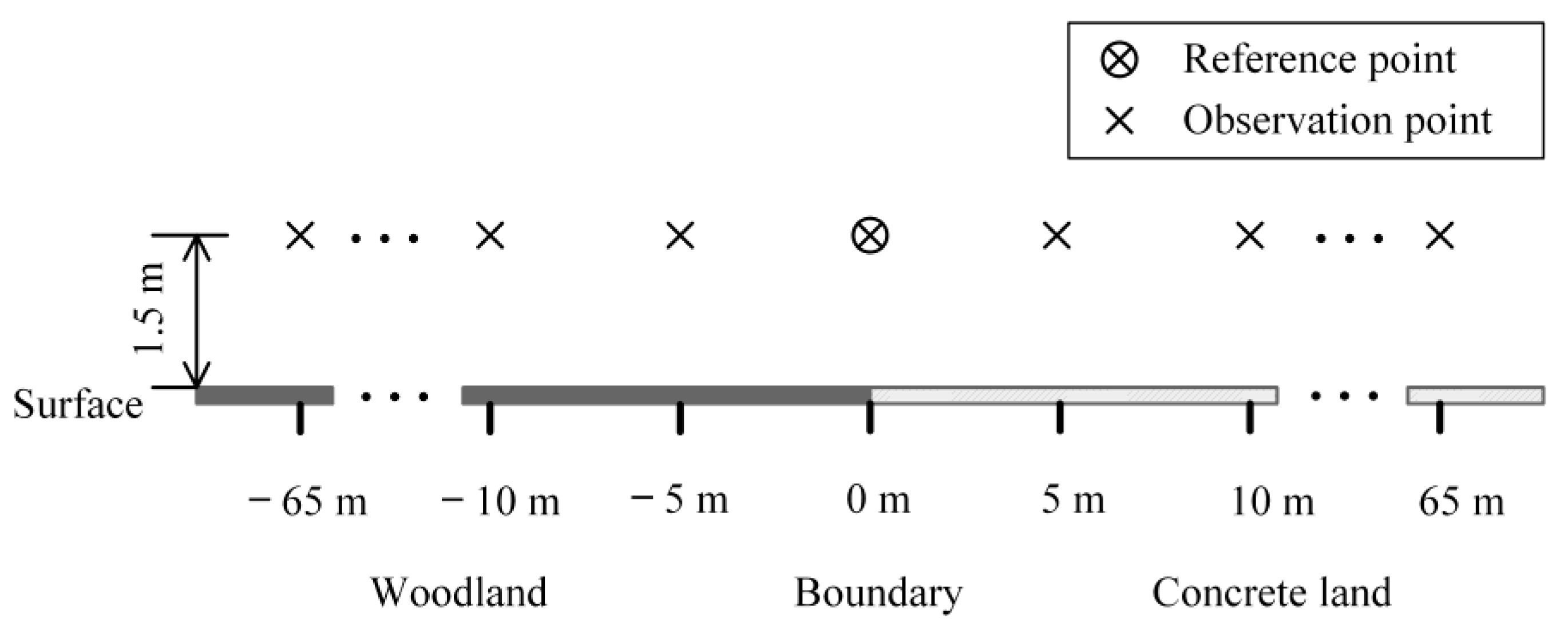
Figure 1. Schematic of the field measurement.
Atmosphere 11 01377 g001
Figure 2. Two priori models for path analysis. (a) Priori model one; (b) Priori model two.
Atmosphere 11 01377 g002
Figure 3. Framework of the genetic support vector regression.
Atmosphere 11 01377 g003
Figure 4. Over flowchart of genetic support vector regression (SVR) training to optimize parameters.
Atmosphere 11 01377 g004
Figure 5. Box plots of Air Temperature Difference (∆Ta) (a) and Relative Humidity Difference (∆RH) (b).
Atmosphere 11 01377 g005
Figure 6. Air Temperature Difference (∆Ta) varying with Distance (∆X) at ∆RH = 0.
Atmosphere 11 01377 g006
Figure 7. Air Temperature Difference (∆Ta) varying with Relative Humidity Difference (∆RH) at ∆X = 0.
Atmosphere 11 01377 g007
Figure 8. Air Temperature Difference (∆Ta) varying with Relative Humidity Difference (∆RH) at ∆X = 30 m.
Atmosphere 11 01377 g008
Table 1. Kruskal–Wallis one-way analysis of variance (ANOVA) of Air Temperature Difference (∆Ta) and Relative Humidity Difference (∆RH) between concrete land and bush woodland.
VariableChi-SquareDFProb (> Chi-Square)
Air Temperature Difference (∆Ta)94.1310.0000
Relative Humidity Difference (∆RH)83.2610.0000
Table 2. Path analysis results of priori model one.
Response VariablePathStandardized Path Coefficientt-StatisticProb (> |t|)R-Square
Air Temperature Difference (∆Ta)Ta ← ∆X 10.1434.1810.0000.870
Ta ← ∆RH−0.822−21.4150.000
Relative Humidity Difference (∆RH)RH ← ∆X−0.740−12.7410.0000.547
1 Representing the path from ∆X to ∆Ta.
Table 3. Path analysis results of priori model two.
Response VariablePathStandardized Path Coefficientt-StatisticProb (> |t|)R-Square
Air Temperature Difference (∆Ta)Ta ← ∆X0.70913.0250.0000.574
Ta ← ∆SPH−0.109−1.7640.040
Specific Humidity Difference (∆SPH)SPH ← ∆X−0.387−4.7760.0000.150
Publisher’s Note: MDPI stays neutral with regard to jurisdictional claims in published maps and institutional affiliations.