Spatial Distribution, Source Apportionment, Ozone Formation Potential, and Health Risks of Volatile Organic Compounds over a Typical Central Plain City in China

Abstract

The profiles, contributions to ozone formation, and associated health risks of 56 volatile organic compounds (VOCs) species were investigated using high time resolution observations from photochemical assessment monitoring stations (PAMs) in Luoyang, China. The daily averaged concentration of total VOCs (TVOCs) was 21.66 ± 10.34 ppbv in urban areas, 14.45 ± 7.40 ppbv in suburbs, and 37.58 ± 13.99 ppbv in an industrial zone. Overall, the VOCs levels in these nine sites followed a decreasing sequence of alkanes > aromatics > alkenes > alkyne. Diurnal variations in VOCs exhibited two peaks at 8:00–9:00 and 19:00–20:00, with one valley at 23:00–24:00. Source apportionment indicated that vehicle and industrial emissions were the dominant sources of VOCs in urban and suburban sites. The industrial site displayed extreme levels, with contributions from petrochemical-related sources of up to 38.3%. Alkenes and aromatics displayed the highest ozone formation potentials because of their high photochemical reactivity. Cancer and noncancer risks in the industrial site were higher than those in the urban and suburban areas, and USEPA possible risk thresholds were reached in the industrial site, indicating PAMs VOC–related health problems cannot be ignored. Therefore, vehicle and industrial emissions should be prioritized when considering VOCs and O₃ control strategies in Luoyang.

1. Introduction

Volatile organic compounds (VOCs) are a variety of organic compounds with a low boiling point and high vapor pressure [1]. VOCs originate from a wide range of sources, including natural (e.g., plant emissions) and anthropogenic sources (e.g., vehicle exhaust emissions and solvent volatilization). VOCs have been reported to be precursors of troposphere ozone (O₃) and secondary organic aerosols (SOA) [2,3,4,5,6]. Moreover, VOCs affect human health [7,8]. For example, VOCs emitted from painting, leather processing, and kitchen cooking can damage the nervous and hematopoietic systems and cause cancers [9,10]. Therefore, a better understanding of the characteristics of VOCs in the atmosphere could offer insights into O₃ pollution, SOA formation, and human health.

Globally, research has focused on two principal aspects of VOCs: the chemical characteristics of VOCs and their effect on O₃ generation and source apportionment of VOCs [11,12,13]. These studies provide data that support the development of O₃ control strategies. For example, Cai et al. [11] determined that alkanes (43%) and aromatics (30%) were the dominant VOCs in Shanghai, and the main sources were vehicle emissions (25%) and solvent volatilization (17%). The VOCs levels have increased in numerous cities in China because of the rapid development of urbanization [14,15]. Alkanes in the Beijing–Tianjin–Hebei region of China were determined to be mostly nonmethane hydrocarbons (NMHCs) (>50%), whereas alkenes and aromatics contribute most to O₃ generation [13]. A similar study in Xi’an reported that vehicle exhaust was the main source of urban VOCs and that alkenes played a dominant role in O₃ generation [16]. However, studies of VOCs in China have focused on developed megacities. Researches on particulate matters for developing areas in China had been started [17,18,19], while for VOCs and O₃ control, data and studies are still leaving limited and far from sufficient [20].

Luoyang is a typical industrial city with a population of more than 7 million, located in Luohe (a tributary of the Yellow River) valley in the North China Plain. Luoyang has long suffered from severe air pollution [21] from various emission sources, such as petrochemical industries, vehicles, and power plants. High VOCs emissions and severe O₃ pollution were observed in Luoyang in 2015 [22]. However, studies on the spatial characteristics of VOCs and their ozone formation potential (OFP) in Luoyang remain limited.

In this study, VOCs sampling was performed four times a day at nine sites (five urban, three suburban, and one industrial) in Luoyang, from 7 to 13 June 2019. Positive matrix factor (PMF) and OFP were used to investigate the sources of VOCs and their effects on O₃ formation. Moreover, the health risks associated with exposure to certain VOCs species were evaluated using the risk model suggested by the United States Environmental Protection Agency (USEPA). The purposes of this study were to 1) determine the characteristics of VOCs and their environmental impacts in Luoyang during summertime, 2) identify sources of VOCs, and 3) assess the health risks associated with VOCs species. These results could provide updated VOCs profile and source information for the government in making VOCs and O₃ control policies.

2. Methodology

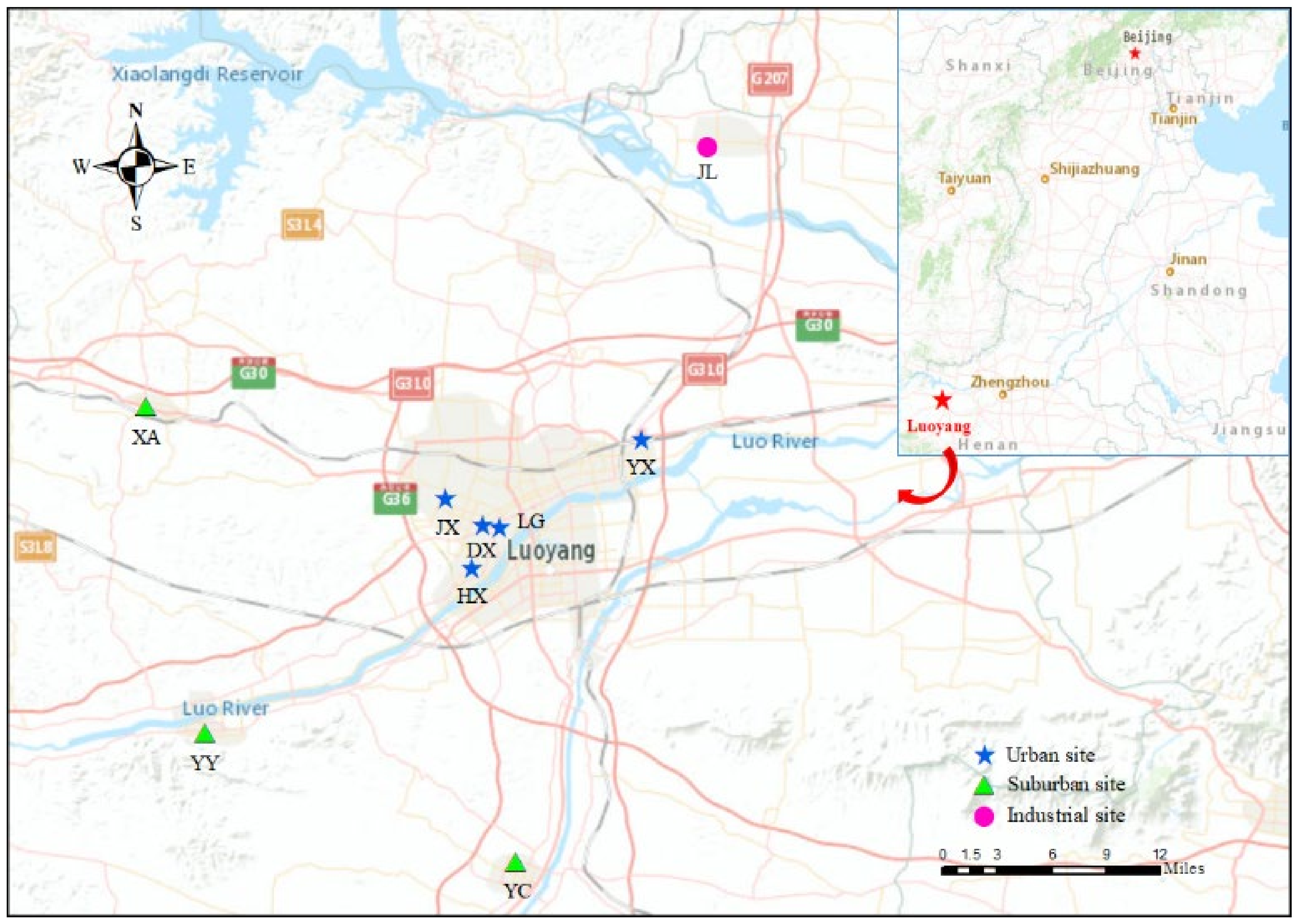
2.1. VOCs Sample Collection

From 7 to 13 June 2019, 1-h VOCs samples were collected four times per day (8:00–9:00, 15:00–16:00, 19:00–20:00, 23:00–24:00, respectively). A total of 252 VOCs samples were collected. Nine sampling sites supported by the National Provincial Air Monitoring Station were selected in this campaign. Five sites are distributed in urban areas: Jianxi District Experimental Primary School (JX), Yuxi Hotel (YX), Luoyang Institute of Technology (LG), Municipal Party School (DX), and Huaxia Road Community (HX). Three sites are distributed in suburban counties: Yiyang County Provincial Control Station (YY), Xin’an County Provincial Control Station (XA), and Yichuan County Experimental Primary School (YC). The last industrial site, Jili District Environmental Protection Agency (JL), is located in the petrochemical base in Luoyang. The geographical distribution of sampling sites is presented in Figure 1, and detailed descriptions of sampling sites are provided in Tables S1 and S2.

A ¼” o.d. stainless-steel multibed adsorbent tube filled with Tenax-TA, Carbograph 1-TD, and Carboxen 1003 (Markes International Ltd., Llantrisant, UK) was employed. A low-flow module pump (ACTI-VOC, Markes International Ltd., Llantrisant, UK) was used to control the flow rate to 50 mL·min⁻¹ for 60 min. Saturated potassium iodide (KI)-coated copper tubes were installed in the air upstream to eliminate the effects of particulate matter and O₃. The sorbent tubes were also precleaned in a thermal conditioner (TC-20, Markes International Ltd., Llantrisant, UK) at 330 °C for 20 min. All preconditioned and sampled tubes were capped and shipped at 0 °C.

2.2. VOCs Analysis

A total of 56 VOCs species identified at photochemical assessment monitoring stations (PAMs) were analyzed using a thermal desorption (TD) unit (Series 2 UNITY-xr system, Markes International Ltd, Llantrisant, UK) coupled with a gas chromatograph/mass spectrometric detector (GC/MSD; Model 7890A/5977B, Agilent, Santa Clara, CA, USA). A tube was connected into the TD unit at room temperature (~25 °C) and purged with ultrahigh purity helium (He) gas at a flow rate of 40 mL·min⁻¹, for detection with GC/MSD. The detailed detection program settings of GC and MSD, including temperature and duration programming, were reported in our previous study [23]. Identification was achieved by comparing the mass spectra and retention times of the chromatographic peaks with those of authentic standards. Certified PAMs standard mixtures (Restek Corporation) were used for calibration. A multipoint calibration curve was established to quantify each of the target compounds with linearity > 0.999. The minimum detection limits (MDLs) for 32 target analytes were in the range of 0.004–0.081 ppbv, with a sampling volume of 3 L (Table S3). Background VOCs samples were also collected and analyzed using the same protocol for quality assurance.

2.3. PMF Source Apportionment Model

The USEPA PMF5.0 model was employed to perform VOCs source apportionment. This model is widely used in this field [12,16,24]. The PMF model can identify the number of emission sources and the species profile in each source and perform source allocation according to the overview of each source and the situation of local emission sources, to obtain the specific allocation ratio of each source. Based on the data matrix X of i by j dimensions (i is the number of samples and j is the VOCs species measured), the calculation principle can be presented as Equation (1).

$$x_{ij}={\displaystyle \sum _{k=1}^p{g}_{ik}{f}_{ki}}+e_{ij}$$

(1)

where x_ij is the jth species concentration measured in the ith sample, g_ik is the species contribution of the kth source to the ith sample, f_kj is the jth species fraction from the kth source, e_ij is the residual for each sample or species, and p is the total number of independent sources. For concentrations higher than MDL, the uncertainty levels were calculated using either Equation (2), otherwise by Equation (3).

$$\mathrm{Uncertainty}=\sqrt{(\mathrm{EF}\times \mathrm{Concertration}{)}^2+{\mathrm{MDL}}^2}$$

(2)

Uncertainty = 0.5 × MDL

(3)

where MDL represents the minimum detection limit (as an absolute concentration value) and EF is the relative measurement error determined through calibration of the instruments (20% in this study). In this study, 32 VOCs species were used as data inputs. The PMF model was run multiple times, extracting four to seven factors, and each run was initialized with different starting points (changing the seed value from 1 to 20). The discussion is based on the seven-factor model resulting from PMF analyses.

2.4. Ozone Formation Potential

The OFP can be calculated based on the maximum incremental reactivity (MIR) [25], as displayed in Equation (4).

OFP = [VOC] × MIR

(4)

where VOC and MIR are the concentration and maximum incremental reactivity of individual VOCs, respectively. The detailed MIRs of each VOC are presented in Table S4.

2.5. Cancer and Noncancer Risk Assessments

Cancer risk from daily exposure of individuals to inhalation can be calculated using Equation (5) [26].

CR = CDI × SF

(5)

where CR is the cancer risk, CDI is the chronic dose of intake by inhalation (mg·kg⁻¹·day⁻¹), and SF is the slope factor of VOCs (kg·day·mg⁻¹). The SFs of main carcinogens were obtained from the Integrated Risk Information System [27]. CDI is affected by many factors and can be calculated using Equation (6).

CDI = C_i × IR × EF × ED / (BW × AL × NY)

(6)

where C_i, IR, EF, ED, BW, AL, and NY represent the contaminant concentration (mg·m⁻³), inhalation rate (m³·h⁻¹), exposure time (h·day⁻¹), total number of exposure days, body weight (kg), average lifetime (year), and total number of days in 1 year (365 day·year⁻¹), respectively. Compounds with cancer risks above 1 × 10⁻⁴ were considered “definite risk,” between 1 × 10⁻⁴ and 1 × 10⁻⁶ were considered “probable risk,” and below 1 × 10⁻⁶ were considered “negligible risk” [28,29].

The noncancer risks of VOCs exposure were quantified as hazard quotients (HQs), which can be calculated using Equation (7).

HQ = ADI/Rfd

(7)

where ADI and RfD are the average daily intake (mg·kg⁻¹·day⁻¹) and reference dose for VOCs species (mg·kg⁻¹·day⁻¹). The RfD values are based on the USEPA [27] and can be calculated using Equation (8).

ADI = (C_i × IR × EF)/BW

(8)

where C_i is the contaminant concentration (mg·m⁻³), IR is the inhalation rate (m³·h⁻¹), EF is the exposure time (h·day⁻¹), and BW is the body weight (kg). HQ ≥ 1.0 indicates adverse health effects in humans [29]. The detailed parameters are presented Tables S5 and S6.

3. Results and Discussion

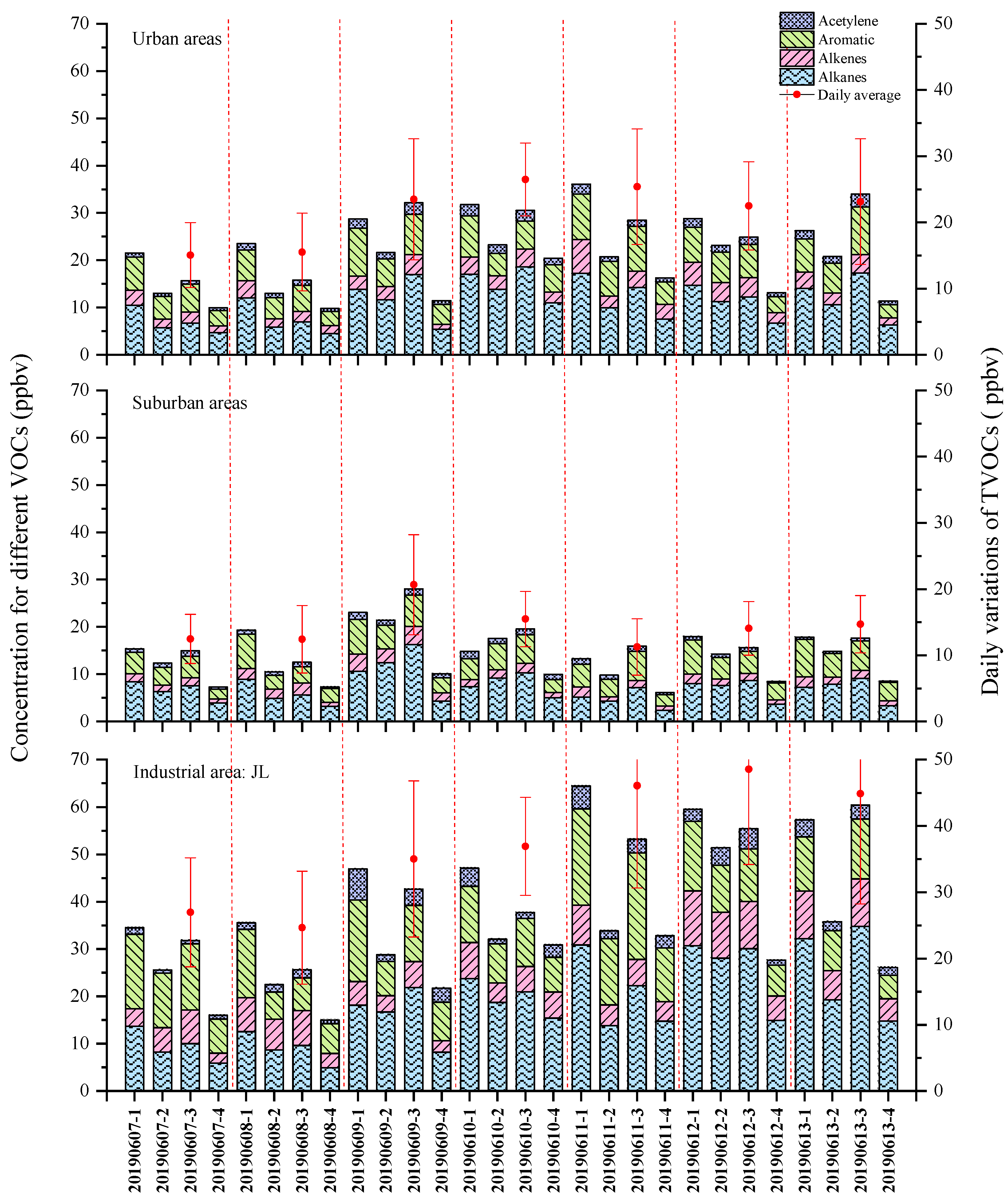
3.1. Characteristics of VOCs and Their Diurnal Variations

The statistical results of the 56 PAMs VOCs species collected from nine sampling sites are presented in

Table 1. The average concentrations of 56 individual VOCs at nine sampling sites in Luoyang, China (ppbv).

	VOCs	JX	YX	LG	DX	HX	YY	XA	YC	JL	VOC-AVG a
Alkane	Ethane	3.91	4.16	2.45	2.64	3.42	2.05	1.71	1.64	5.09	3.01
	Propane	4.25	6.02	1.20	1.34	3.03	2.94	1.99	1.74	4.85	3.04
	Isobutane	1.06	1.07	0.61	0.50	0.68	0.49	0.53	0.50	1.34	0.75
	n-Butane	1.08	1.35	0.56	0.58	0.86	1.15	0.57	0.62	1.17	0.88
	iso-Pentane	0.66	0.79	0.22	0.25	0.41	0.02	0.02	0.02	0.83	0.36
	n-Pentane	0.68	0.60	0.27	0.24	0.37	0.24	0.24	0.24	0.71	0.40
	Cyclopentane	0.05	0.21	0.12	0.12	0.23	0.14	0.14	0.12	0.08	0.13
	2,2-Dimethylbutane	0.04	0.05	0.03	0.03	0.03	0.03	0.03	0.02	0.08	0.04
	2,3-Dimethylbutane	0.04	0.08	0.02	0.02	0.02	0.02	0.02	0.02	0.08	0.04
	2-Methylpentane	0.31	0.32	0.18	0.12	0.12	0.20	0.18	0.21	0.39	0.23
	3-Methylpentane	0.24	0.36	0.12	0.10	0.14	0.15	0.14	0.16	0.28	0.19
	n-Hexane	0.49	0.41	0.12	0.11	0.16	0.16	0.26	0.17	1.36	0.36
	2,4-Dimethylpentane	0.03	0.03	0.02	0.02	0.02	0.02	0.02	0.02	0.04	0.02
	Methylcyclopentane	0.07	0.10	0.03	0.04	0.04	0.04	0.05	0.05	0.11	0.06
	2-Methylhexane	0.08	0.09	0.04	0.04	0.04	0.05	0.05	0.05	0.09	0.06
	2,3-Dimethylpentane	0.08	0.07	0.04	0.04	0.04	0.06	0.07	0.06	0.09	0.06
	Cyclohexane	0.27	0.15	0.08	0.07	0.09	0.15	0.22	0.20	0.46	0.19
	3-Methylhexane	0.10	0.24	0.11	0.12	0.09	0.08	0.08	0.08	0.14	0.12
	n-Heptane	0.09	0.15	0.04	0.06	0.05	0.04	0.03	0.03	0.12	0.07
	Methylcyclohexane	0.07	0.13	0.06	0.05	0.06	0.04	0.04	0.05	0.10	0.07
	2,3,4-Trimethylpentane	0.02	0.02	0.01	0.02	0.01	0.01	0.01	0.01	0.02	0.01
	2,2,4-Trimethylpentane	0.03	0.03	0.03	0.04	0.03	0.02	0.01	0.02	0.04	0.03
	2-Methylheptane	0.02	0.02	0.02	0.02	0.02	0.01	0.01	0.01	0.03	0.02
	3-Methylheptane	0.02	0.02	0.02	0.02	0.02	0.01	0.01	0.01	0.02	0.02
	n-Octane	0.05	0.05	0.03	0.03	0.03	0.04	0.03	0.03	0.06	0.04
	n-Nonane	0.07	0.08	0.05	0.06	0.06	0.04	0.04	0.04	0.10	0.06
	n-Decane	0.07	0.10	0.06	0.09	0.06	0.05	0.05	0.04	0.09	0.07
	Undecane	0.10	0.09	0.10	0.20	0.04	0.05	0.06	0.06	0.17	0.10
	Dodecane	0.04	0.06	0.09	0.13	0.05	0.07	0.07	0.06	0.05	0.07
Alkene	Ethylene	2.26	2.75	1.25	1.98	2.18	1.48	1.09	1.17	4.23	2.04
	Propylene	0.71	1.16	0.24	0.20	0.37	0.21	0.21	0.21	0.91	0.47
	trans-2-Butene	0.03	0.06	0.03	0.03	0.02	0.02	0.02	0.02	0.08	0.03
	1-Butene	0.06	0.06	0.04	0.04	0.03	0.07	0.07	0.07	0.11	0.06
	cis-2-Butene	0.17	0.28	0.05	0.05	0.11	0.05	0.06	0.06	0.53	0.15
	1-Pentene	0.05	0.05	0.04	0.03	0.11	0.06	0.07	0.08	0.06	0.06
	trans-2-Pentene	0.05	0.10	0.02	0.04	0.03	0.01	0.02	0.00	0.09	0.04
	cis-2-Pentene	0.03	0.08	0.00	0.01	0.01	0.01	0.01	0.00	0.06	0.02
	1-Hexene	0.02	0.02	0.02	0.02	0.01	0.01	0.01	0.02	0.02	0.02
	Isoprene	0.02	0.02	0.04	0.03	0.03	0.05	0.05	0.05	0.02	0.04
Aromatic	Benzene	1.52	0.78	0.95	0.86	0.95	1.77	0.51	0.24	2.87	1.16
	Toluene	4.22	3.03	2.67	3.65	4.02	5.59	1.74	0.83	5.24	3.44
	Ethylbenzene	0.69	0.49	0.34	0.34	0.24	0.40	0.27	0.26	0.89	0.44
	m-/p-Xylene	0.83	0.71	0.33	0.30	0.25	0.40	0.33	0.31	0.85	0.48
	o-Xylene	0.62	0.35	0.22	0.21	0.18	0.24	0.17	0.15	0.53	0.30
	Styrene	0.42	0.18	0.13	0.12	0.11	0.08	0.17	0.09	0.41	0.19
	Isopropylbenzene	0.02	0.04	0.01	0.03	0.01	0.01	0.01	0.01	0.02	0.02
	n-Propylbenzene	0.02	0.03	0.02	0.02	0.03	0.01	0.02	0.01	0.02	0.02
	m-Ethyltoluene	0.04	0.05	0.05	0.04	0.04	0.03	0.03	0.02	0.05	0.04
	p-Ethyltoluene	0.04	0.04	0.03	0.03	0.04	0.02	0.02	0.02	0.05	0.03
	1,3,5-Trimethylbenzene	0.03	0.04	0.03	0.03	0.03	0.02	0.02	0.02	0.03	0.03
	o-Ethyltoluene	0.03	0.04	0.02	0.03	0.02	0.04	0.02	0.02	0.03	0.03
	1,2,4-Trimethylbenzene	0.07	0.08	0.06	0.06	0.06	0.04	0.04	0.04	0.08	0.06
	1,2,3-Trimethylbenzene	0.02	0.03	0.02	0.02	0.03	0.01	0.02	0.02	0.03	0.02
	m-Diethylbenzene	0.02	0.06	0.02	0.02	0.02	0.02	0.01	0.02	0.02	0.02
	p-Diethylbenzene	0.03	0.05	0.05	0.05	0.05	0.03	0.03	0.03	0.03	0.04
Acetylene	Acetylene	1.80	1.81	1.10	1.03	1.18	2.15	0.32	0.06	2.33	1.31
	TVOCs	27.81	29.21	14.49	16.38	20.39	21.22	12.01	10.12	37.58	21.02
	TAVG b	21.66					14.45			37.58

Note: ^a is the total average concentration of the individual VOCs among nine sampling sites; ^b is the total average concentration of urban, suburban and industrial sampling sites.

. Among the nine monitoring sites, the highest daily averaged concentration of TVOCs (total VOCs, sum of the 56 measured species) was observed in JL (37.58 ± 13.99 ppbv), followed by YX (29.21 ± 11.15 ppbv), JX (27.81 ± 11.09 ppbv), YY (21.22 ± 7.79 ppbv), HX (20.39 ± 7.75 ppbv), DX (16.38 ± 5.66 ppbv), LG (14.49 ± 5.33 ppbv), XA (12.01 ± 4.36 ppbv), and YC (10.12 ± 3.97 ppbv). JL is located at the petrochemical base in Luoyang and thus expected to display the highest VOCs levels, with the highest concentration of ethylene, n-hexane, trans-2-butene, toluene, and xylene, which are characteristic of the petroleum refining process [30,31,32]. The average daily concentration of TVOCs was determined to be 21.66 ± 10.34 ppbv in urban areas and 14.45 ± 7.40 ppbv in the suburbs. The difference between the urban and suburban concentrations was principally related to the larger population, and consequently, higher human activity in urban areas. However, the spatial distribution differences within urban (suburban) areas were very high, with over 100% difference observed between YX and LG in urban areas and between YY and YC in suburban areas, which indicated that the district-scale environment had a nonnegligible effect on TVOCs distributions [12]. As illustrated in Table 1, the four species with the highest daily averaged concentrations (9 sites average), namely toluene (3.44 ± 2.25 ppbv), propane (3.04 ± 2.58 ppbv), ethane (3.01 ± 2.08ppbv), and ethylene (2.04 ± 1.36 ppbv), accounted for over 50% of TVOCs, indicating the significant contribution of vehicle emissions [33].

The measured 56 PAMs VOCs were classified into four categories: alkanes, alkenes, aromatics, and acetylene (Table S7). Overall, the daily averaged concentrations were in the order of alkanes > aromatics > alkenes > alkyne. The highest alkane proportions in TVOCs were determined to be approximately 50% in urban, suburban, and industrial sites. The concentration of all categories of VOCs in JL was almost 2–3 times higher than those in urban and suburban sites, indicating that JL may suffer from extremely high VOCs pollution. The alkanes that displayed the highest proportions were ethane, propane, and ethylene, which are widely reported in vehicle exhaust and natural gas [34,35]. Abundant toluene (accounting for 39.6–66.0% in aromatics) was observed among the nine sampling sites. The sources of toluene are varied, such as vehicle emissions, solvent usage, and petrochemical processes [31,35,36]. The findings indicated that VOCs emissions in Luoyang were complex.

Table 2. Diurnal variations of TVOCs at nine sampling sites in Luoyang, China (ppbv).

	8:00–9:00	15:00–16:00	19:00–20:00	23:00–24:00	Site–AVG a
Urban area	28.10	19.38	25.93	13.21	21.66
JX	36.85	26.52	33.02	14.85	27.81
YX	38.57	24.74	34.17	19.37	29.21
LG	18.56	12.72	17.64	9.05	14.49
DX	21.17	14.40	19.55	10.40	16.38
HX	25.35	18.51	25.28	12.40	20.39
Suburbs	17.40	14.40	17.75	8.26	14.45
YY	25.83	20.78	25.96	12.31	21.22
XA	14.38	12.14	14.67	6.85	12.01
YC	11.98	10.27	12.61	5.62	10.12
Industrial site (JL)	49.33	32.85	43.85	24.30	37.58
Period-AVG b	26.74	19.19	25.10	12.74

Note: ^a is the daily average concentration of a sampling site. ^b is the total average concentration in a specific time period among nine sampling sites.

presents a summary of the average diurnal variations in VOCs levels in different sampling sites. TVOCs generally displayed higher concentrations in the morning (8:00–9:00; 28.10 ± 10.16 ppbv for urban, 17.40 ± 7.07 ppbv for suburbs, 49.33 ± 11.66 ppbv for JL) and evening (23:00–24:00; 25.93 ± 10.34 ppbv for urban, 17.75 ± 8.12 ppbv for suburbs, 43.85 ± 12.99 ppbv for JL) and lower concentrations at midnight (23:00–24:00; 13.21 ± 5.69 ppbv for urban, 8.26 ± 3.36 ppbv for suburbs, 24.30 ± 6.99 ppbv for JL). Figure 2 illustrates the averaged diurnal patterns of four categories (alkanes, alkenes, aromatics, and acetylenes) of VOCs in urban and suburban sampling sites. Alkanes, alkenes, aromatics, and acetylenes displayed similar diurnal patterns to the TVOCs. The relatively high TVOCs levels in the morning and evening periods could be mainly attributed to the high human activity (i.e., rush hour traffic) [37]. The reasons of the lowest TVOCs concentrations in midnight were dispersion and dilution of the pollutants, which is highly correlated with the consumption of VOCs in the dark reaction processes and extremely low human activities [38]. VOCs were systematically higher in JL because this sampling site is located in an urban area with abundant industries.

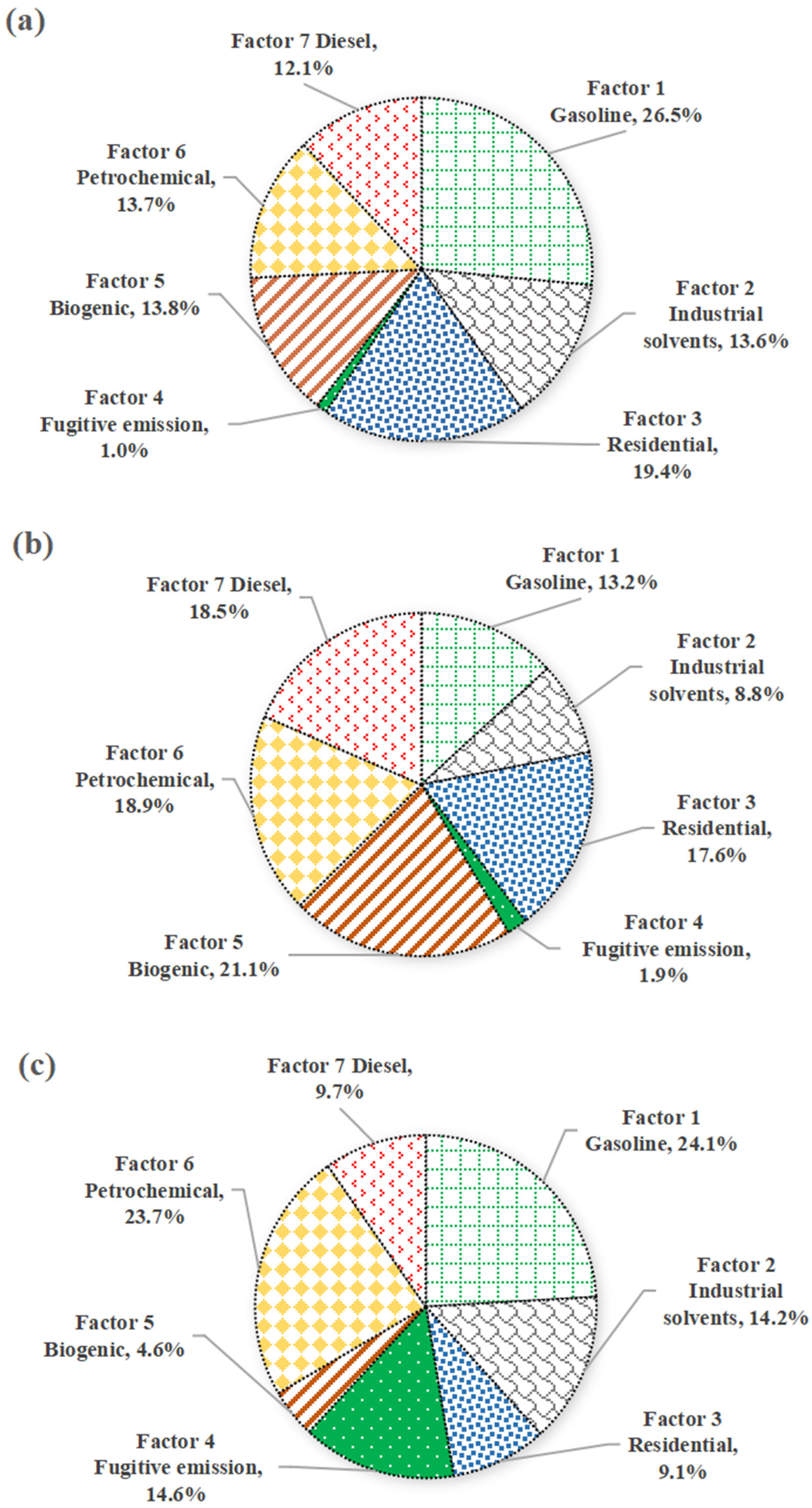
3.2. VOC Source Apportionment

VOC source apportionments were performed in urban, suburban, and industrial areas of Luoyang by using the PMF model. A 7-factor PMF solution was selected as the optimal representation of the VOC sources and source profiles of urban sites, as illustrated in Figure S1. The key characteristic species identified in factor 1 were C3–C5 alkanes (especially isopentane), ethylene, propylene, benzene, toluene, and acetylene. These short-chain alkanes, alkenes, and acetylene are usually associated with unburned vehicular emissions, and propylene is reported to be a typical product of internal combustion engines [12,39,40,41]. Toluene is also related to gasoline emissions [35,36], and the toluene/benzene ratio was 1.9, which accords with the vehicle exhaust range indicator of 1.5–3.0 [42,43]. Therefore, factor 1 could be interpreted as gasoline exhaust. Factor 2 was characterized by a significant number of aromatics, such as benzene, toluene, ethylbenzene, and xylene. These aromatics are mainly released from solvent usage [36,44,45,46,47], and benzene and toluene are also emitted from industrial sources [40,46,48], indicating that this group could be considered industrial solvents. Factor 3 was rich in low-carbon alkanes and alkenes with some aromatics. Ethane, propane, ethylene, ethyne, and benzene are the major indicators of natural gas and coal combustion [34,49,50]. Moreover, certain residential activities (e.g., cooking) also release abundant aromatics [23]. Factor 3 can be thus considered a residential source. Factor 4 was rich in iso-butane/n-butane and iso-pentane/n-pentane, which are representative tracers of gasoline evaporation, and thus indicate fugitive emission [46,48,51,52]. Factor 5 can be considered a biogenic source because of high isoprene, which is a typical tracer of biogenic emission [53,54]. Factor 6 displayed relatively high abundances of n-hexane, ethylene, trans-2-butene, toluene, and xylene, which are features of the petroleum refining process. Factor 6 was thus associated with a petrochemical source [30,31,32]. Factor 7 was rich in undecane and dodecane, which are tracers for diesel combustion [35,36], and thus regard as diesel vehicular emissions. The source apportionments in the suburban and industrial areas were similar to the source apportionment in the urban areas. However, the sequences differed, as illustrated in Figures S2 and S3.

The source contributions toward TVOCs in the urban, suburban, and industrial areas are plotted in Figure 3. Overall, the contributions of each source were similar in the urban and suburban areas but considerably different in the industrial area. Vehicle emission (the sum of gasoline and diesel exhaust, accounting for 38.6% and 31.7% in the urban and suburban areas, respectively) was the main source of ambient VOCs in Luoyang, because of the large amount of vehicle traffic in Luoyang (1.32 million vehicles in 2019). Similar results were reported in other cities in China [16,55]. Moreover, industrial emission (the sum of industrial solvents and petrochemical emission, accounting for 27.3% and 27.7% in urban and suburban, respectively) was the second-highest contributor. The contribution of petrochemicals was higher in the suburbs than in the urban area because of the larger number of petrochemical plants located in suburban areas according to Luoyang’s Statistical Year Book 2018 [56]. The contributions of residential sources were slightly higher in the urban area (19.4%) than in the suburban area (17.6%) because of the high population density and intense human activity in the urban area. Furthermore, the contributions of vegetation cannot be neglected and were higher in suburban (21.1%) than in urban (13.8%) areas, because the suburban sampling sites are mainly located in areas with rich vegetation. A special case can be seen in JL that the contributions of petrochemical and fugitive emissions were as high as 23.7% and 14.6%, respectively. The petrochemical base located in JL is large and produces chemical products of petroleum and crude oil, which explains the higher contribution of petrochemical-related sources (the sum of petrochemical and fugitive emissions, 38.3%) compared with urban and suburban areas. In general, urban and suburban areas should mainly focus on reducing pollution emissions from traffic sources, and JL needs to formulate strict emission control policies and improve the process management for the local petrochemical industry.

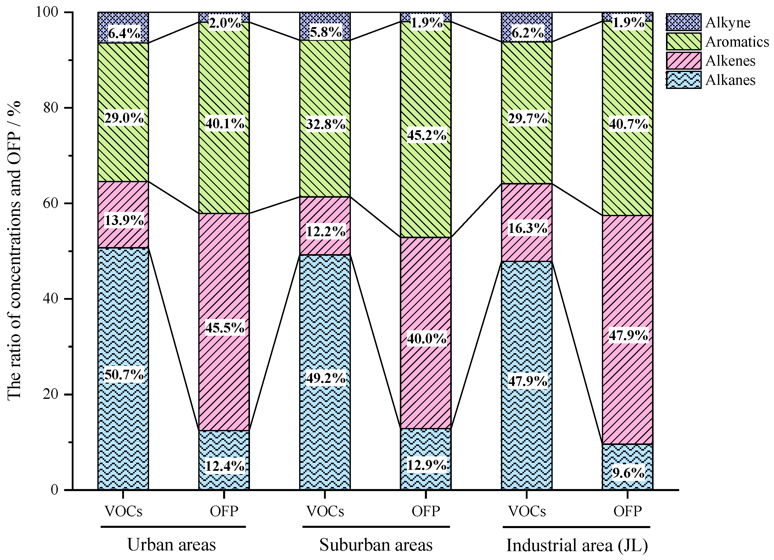
3.3. Ozone Formation Potential

The average concentrations and OFP proportions of the four categories (alkanes, alkenes, aromatics, and acetylene) and the OFP values in urban, suburban, and industrial sites are reported in Figure 4 and Table S8, respectively. The OFP generally followed the sequence of alkenes (aromatics) > alkanes > alkynes, and the OFP in the industrial area was almost 2–3 times higher than in urban and suburban areas. Moreover, high OFP values were observed in JX and YX, which was closely related to their relatively high VOCs emissions. Although alkenes accounted for only 12.2–16.3% of the TVOCs, they were the relatively large contributors to OFP (40.0–47.9%), mainly because of their high reactivity [57]. Aromatics also contributed up to 40.1–45.2% of the total OFP with 29.0–32.8% mass contribution to the TVOCs, because of the high concentration of aromatics and high reactivity. Alkanes displayed the highest TVOCs occupation (49.8%) but the lowest OFP proportion (12.3%), suggesting a limited role in photochemical reactions and O₃ formation. Therefore, alkenes and aromatics should be preferentially considered in regional O₃ control strategy development.

The ten highest OFP of the VOCs species, determined using the MIR method, are listed in

Table 3. The top ten VOCs species for OFP in urban, suburban and industrial areas (ppbv).

Urban Areas			Suburban Areas			Industrial Area
VOCs	OFP	OFP Ratio	VOCs	OFP	OFP Ratio	VOCs	OFP	OFP Ratio
Ethylene	18.26	29.1%	Ethylene	10.92	26.8%	Ethylene	37.02	32.3%
Toluene	13.65	21.7%	Toluene	10.55	25.9%	Toluene	20.33	17.7%
Propylene	6.07	9.7%	m-/p-Xylene	3.30	8.1%	Propylene	10.35	9.0%
m-/p-Xylene	4.59	7.3%	Propylene	2.38	5.8%	m-/p-Xylene	8.08	7.0%
o-Xylene	2.34	3.7%	o-Xylene	1.39	3.4%	cis-2-Butene	7.42	6.5%
cis-2-Butene	1.82	2.9%	Propane	1.02	2.5%	o-Xylene	3.93	3.4%
Propane	1.46	2.3%	Ethylbenzene	0.91	2.2%	Ethylbenzene	2.62	2.3%
Acetylene	1.29	2.0%	n-Butane	0.84	2.1%	Propane	2.23	1.9%
Ethylbenzene	1.24	2.0%	Acetylene	0.79	1.9%	Acetylene	2.17	1.9%
n-Butane	0.96	1.5%	cis-2-Butene	0.77	1.9%	Benzene	1.98	1.7%

, and the urban, suburban, and industrial areas displayed similar characteristics. These ten VOCs species accounted for less than 60% of the TVOCs but contributed over 80% of the total OFP, which indicates that controlling the key VOCs species plays a vital role in reducing the O₃ level. Ethylene and toluene contributed most of the OFP. These species can be derived from combustion-related sources, such as vehicle emissions, natural gas, and coal combustions [12,34,40,49,50]. The diurnal variations of concentration in ethylene and toluene are plotted in Figure S4, and two peaks can be seen in the morning and evening, indicating that the emissions are closely related to human activity. These findings and the previous source analysis indicate that vehicle emissions were likely to be the largest contributors to OFP in Luoyang. Therefore, strengthening vehicle exhaust purification and vehicle quantity management measures should be effective in reducing O₃ levels in Luoyang.

3.4. Cancer and Noncancer Risk Assessments

The results of the cancer and noncancer risk assessments from average daily exposure to six common aromatic hydrocarbons of PAMs are presented in

Table 4. Cancer and non-cancer risk assessment of VOCs in urban, suburban and industrial areas.

VOCs	Non-Cancer Risk-HQ			Cancer Risk-CR
	Urban Area	Suburbs	JL	Urban Area	Suburbs	JL
Benzene	0.494	0.409	1.399	6.7 × 10−7	5.6 × 10−7	1.9 × 10−6
Toluene	0.101	0.078	0.151	-	-	-
Ethylbenzene	0.011	0.008	0.024	1.1 × 10−7	8.4 × 10−8	2.4 × 10−7
m-/p-Xylene	0.006	0.005	0.011	-	-	-
o-Xylene	0.004	0.002	0.007	-	-	-
Styrene	0.002	0.001	0.005	3.3 × 10−9	2.0 × 10−9	7.1 × 10−9
SUM	0.619	0.504	1.597	7.9 × 10−7	6.4 × 10−7	2.2 × 10−6

. The total noncancer risk of JL (1.597) was almost three times higher than the noncancer risks in urban (0.619) and suburban sites (0.504) and exceeded the safe threshold of 1, indicating that long-term exposure to these VOCs would harm the human health. Notably, benzene (0.494 for urban, 0.409 for suburbs, and 1.399 for JL) was responsible for over half of the risk caused by the six measured VOCs. Benzene is mainly emitted from vehicles, industrial solvents, and petrochemical sources. Similarly, the total cancer risk was higher in JL (2.2 × 10⁻⁶) than in the urban (7.9 × 10⁻⁷) and suburban sites (6.4 × 10⁻⁷) and exceeded the risk threshold (10⁻⁶) established by the USEPA. Benzene was also the dominant contributor to the total cancer risks among the VOCs. Therefore, benzene emissions should be prioritized when managing the noncancer and cancer risks in PAMs. Although cancer and noncancer risks at the urban and suburban sites did not reach the risk threshold, the risk of VOCs cannot be neglected for the following reasons: 1) the risk of PAMs and the harm of exposure from other VOCs (e.g., halohydrocarbon) is also significant, and 2) the concentration of VOCs in a specific space (e.g., factory, kitchen) is higher than the ambient concentration. For example, both the noncancer risk and cancer risk of ambient VOCs (benzene, carbon tetrachloride, trichloromethane, and 1,2-dichloroethane) exceeded the acceptable threshold specified for adults, suggesting an obvious risk in Hefei, China [58]. Sun et al. [23] indicated that the risk assessment of kitchen VOCs in the Guanzhong Plain area far exceeds the safety threshold; therefore, the superimposed concentrations in other environments cannot be ignored.

4. Conclusions

High time resolution observations of 56 PAMs VOCs species were performed in Luoyang, China. The daily averaged concentration of TVOCs was 21.66 ± 10.34 ppbv in urban areas, 14.45 ± 7.40 ppbv in suburban areas, and 37.58 ± 13.99 ppbv in the industrial site. Diurnal variations were observed, with VOCs levels peaking in the morning and evening and dipping at midnight, which may reflect human activities and photochemical reactions in urban, suburban, and industrial sites. The source apportionment results indicated that vehicle and industrial emissions were the two dominant sources of VOCs in Luoyang, whereas other sources displayed different contributions in urban and suburban areas. Marginally higher contributions from residential sources were observed in urban areas (19.4%) than in suburban areas (17.6%), whereas the biogenic contributions were 13.8% and 21.1% in the urban and suburban areas, respectively. The highest contribution from petrochemical-related sources (the sum of petrochemical and fugitive emission: 38.3%) was observed in JL. The OFP evaluation results confirmed that alkenes and aromatics were the largest contributors to OFP. Ethylene and toluene were responsible for the majority of the OFP. Therefore, controlling vehicle emission would have a considerable effect on O₃ pollution control. The health assessment results revealed that the cancer and noncancer risks in the JL were substantially higher than those in the urban and suburban areas, and the industrial levels reached the possible risk threshold defined by USEPA. The findings indicate that vehicle and industrial emissions should be preferentially controlled in regional VOCs control policies to reduce health damages in Luoyang, China. The halogenated VOC levels and the associated health risks will be investigated in the future.

References

1. Kountouriotis, A.; Aleiferis, P.G.; Charalambides, A.G. Numerical investigation of VOC levels in the area of petrol stations. Sci. Total Environ. 2014, 470, 1205–1224. [Google Scholar] [CrossRef] [PubMed] [Green Version]
2. Hsu, C.Y.; Chiang, H.C.; Shie, R.H.; Ku, C.H.; Lin, T.Y.; Chen, M.J.; Chen, N.T.; Chen, Y.C. Ambient VOCs in residential areas near a large-scale petrochemical complex: Spatiotemporal variation, source apportionment and health risk. Environ. Pollut. 2018, 240, 95–104. [Google Scholar] [CrossRef] [PubMed]
3. McFiggans, G.; Mentel, T.F.; Wildt, J.; Pullinen, I.; Kang, S.; Kleist, E.; Schmitt, S.; Springer, M.; Tillmann, R.; Wu, C.; et al. Secondary organic aerosol reduced by mixture of atmospheric vapours. Nature 2019, 565, 587–593. [Google Scholar] [CrossRef] [PubMed]
4. Sillman, S. The relation between ozone, NOx and hydrocarbons in urban and polluted rural environments. Atmos. Environ. 1999, 33, 1821–1845. [Google Scholar] [CrossRef]
5. Toro, M.V.; Cremades, L.V.; Calbó, J. Relationship between VOC and NOx emissions and chemical production of tropospheric ozone in the Aburra Valley (Colombia). Chemosphere 2006, 65, 881–888. [Google Scholar] [CrossRef] [PubMed]
6. Zhang, Q.; Yuan, B.; Shao, M.; Wang, X.; Liu, S. Variations of ground-level O3 and its precursors in Beijing in summertime between 2005 and 2011. Atmos. Chem. Phys. 2013, 14, 6089–6101. [Google Scholar] [CrossRef] [Green Version]
7. Zhao, H.; Zheng, Y.F.; Li, S.; Xu, J.X.; Guan, Q. Long Term Variations of Ozone Concentration of in a Winter Wheat Field and Its Loss Estimate Based on Dry Matter and Yield. Huan Jing Ke Xue. 2017, 38, 5315–5325. (In Chinese) [Google Scholar]
8. Kampa, M.; Castanas, E. Human health effects of air pollution. Environ. Pollut. 2008, 151, 362–367. [Google Scholar] [CrossRef]
9. Agency for Toxic Substances and Disease Registry (ATSDR). 2011. Available online: http://www.atsdr.cdc.gov (accessed on 11 May 2016).
10. International Agency for Research on Cancer (IARC). 2015. Available online: http://monographs.iarc.fr/ENG/Classification/latest_classif.php (accessed on 11 May 2016).
11. Cai, C.; Geng, F.; Tie, X.; Yu, Q.; An, J. Characteristics and source apportionment of VOCs measured in Shanghai, China. Atmos. Environ. 2010, 44, 5005–5014. [Google Scholar] [CrossRef]
12. Jing, L.; Zhai, C.; Yu, J.; Liu, R.; Li, Y.; Zeng, L.; Xie, S. Spatiotemporal variations of ambient volatile organic compounds and their sources in Chongqing, a mountainous megacity in China. Sci. Total Environ. 2018, 627, 1442–1452. [Google Scholar]
13. Li, L.; Xie, S.; Zeng, L.; Wu, R.; Li, J. Characteristics of volatile organic compounds and their role in ground-level ozone formation in the Beijing-Tianjin-Hebei region, China. Atmos. Environ. 2015, 113, 247–254. [Google Scholar] [CrossRef]
14. Li, K.; Jacob, D.J.; Liao, H.; Shen, L.; Zhang, Q.; Bates, K.H. Anthropogenic drivers of 2013–2017 trends in summer surface ozone in China. Proc. Natl. Acad. Sci. USA 2019, 116, 422–427. [Google Scholar] [CrossRef] [PubMed] [Green Version]
15. Liu, S.; Xing, J.; Zhang, H.; Ding, D.; Wang, S. Climate-driven trends of biogenic volatile organic compound emissions and their impacts on summertime ozone and secondary organic aerosol in China of the 2050s. Atmos. Environ. 2019, 218, 117020. [Google Scholar] [CrossRef]
16. Sun, J.; Shen, Z.X.; Zhang, Y.; Zhang, Z.; Li, X. Urban VOC profiles, possible sources, and its role in ozone formation for a summer campaign over Xi’an, China. Environ. Sci. Pollut. Res. 2019, 26, 27769–27782. [Google Scholar] [CrossRef] [PubMed]
17. Geng, N.B.; Wang, J.; Xu, Y.F.; Zhang, W.D.; Chen, C.; Zhang, R.Q. PM2.5 in an industrial district of Zhengzhou, China: Chemical composition and source apportionment. Particuology 2013, 11, 99–109. [Google Scholar] [CrossRef]
18. Lei, Y.L.; Shen, Z.X.; Tang, Z.Y.; Zhang, Q.; Sun, J.; Ma, Y.J.; Wu, X.Y.; Qin, Y.M.; Xu, H.M.; Zhang, R.J. Aerosols chemical composition, light extinction, and source apportionment near a desert margin city, Yulin, China. PeerJ 2019, 8, 8447. [Google Scholar] [CrossRef] [PubMed]
19. Zhan, C.L.; Zhang, J.Q.; Zheng, J.R.; Yao, R.Z.; Wang, P.; Liu, H.X.; Xiao, W.S.; Liu, X.L.; Cao, J.J. Characterization of carbonaceous fractions in PM2.5 and PM10 over a typical industrial city in central China. Environ. Sci. Pollut. Res. 2019, 26, 16855–16867. [Google Scholar] [CrossRef]
20. Xu, Y.; Ying, Q.; Hu, J.; Gao, Y.; Yang, Y.; Wang, D.; Zhang, H. Spatial and temporal variations in criteria air pollutants in three typical terrain regions in Shaanxi, China, during 2015. Air Qual. Atmos. Hlth. 2017, 11, 95–109. [Google Scholar] [CrossRef]
21. Zhang, Y.P.; Jun-Liang, X.U.; Zhao, X.P.; Wang, D.G. Grey Correlation Analysis of Air Quality and Its Affection Factors in Luoyang City. J. Henan Univ. Sci. Technol. 2012, 44, 100–104. [Google Scholar]
22. Gu, X.; Yin, S.; Lu, X.; Zhang, H.; Wang, L.; Bai, L.; Wang, C.; Zhang, R.; Yuan, M. Recent development of a refined multiple air pollutant emission inventory of vehicles in the Central Plains of China. J. Environ. Sci. 2019, 84, 80–96. [Google Scholar] [CrossRef]
23. Sun, J.; Shen, Z.X.; Zhang, L.M.; Zhang, Y.; Zhang, T.; Lei, Y.L.; Niu, X.Y.; Zhang, Q.; Dang, W.; Han, W.P.; et al. Volatile organic compounds emissions from traditional and clean domestic heating appliances in Guanzhong Plain, China: Emission factors, source profiles, and effects on regional air quality. Environ. Int. 2019, 133, 105252. [Google Scholar] [CrossRef] [PubMed]
24. Su, Y.C.; Chen, W.H.; Fan, C.L.; Tong, Y.H.; Weng, T.H.; Chen, S.P.; Kuo, C.P.; Wang, J.L.; Chang, J.S. Source Apportionment of Volatile Organic Compounds (VOCs) by Positive Matrix Factorization (PMF) supported by Model Simulation and Source Markers-Using Petrochemical Emissions as a Showcase. Environ. Pollut. 2019, 254, 112848. [Google Scholar] [CrossRef] [PubMed]
25. Carter, W.P. Updated Maximum Incremental Reactivity Scale and Hydrocarbon Bin Reactivities for Regulatory Applications; California Air Resources Board Contract; University of California: Riverside, CA, USA, 2009; Volume 339. [Google Scholar]
26. Huang, Y.; Ho, S.S.H.; Ho, K.F.; Lee, S.C.; Yu, J.Z.; Louie, P.K.K. Characteristics and health impacts of VOCs and carbonyls associated with residential cooking activities in Hong Kong. J. Hazardous Mater. 2011, 186, 344–351. [Google Scholar] [CrossRef] [PubMed]
27. USEPA. Integrated Risk information Systemd-Benzene. 1998. Available online: http://www.epa.gov/iris/subst.o276.htm (accessed on 14 December 2020).
28. An, T.; Huang, Y.; Li, G.; He, Z.; Chen, J.; Zhang, C. Pollution profiles and health risk assessment of VOCs emitted during e-waste dismantling processes associated with different dismantling methods. Environ. Int. 2014, 73, 186–194. [Google Scholar] [CrossRef]
29. He, Z.; Li, G.; Chen, J.; Huang, Y.; An, T.; Zhang, C. Pollution characteristics and health risk assessment of volatile organic compounds emitted from different plastic solid waste recycling workshops. Environ. Int. 2015, 77, 85–94. [Google Scholar] [CrossRef]
30. Cui, H. Source Profile of Volatile Organic Compounds (VOCs) of a Petrochemical Industry in the Yangtze River Delta, China. Chem. Eng. Trans. 2016, 54, 121–126. [Google Scholar]
31. Cetin, E.; Odabasi, M.; Seyfioglu, R. Ambient volatile organic compound (VOC) concentrations around a petrochemical complex and a petroleum refinery. Sci. Total Environ. 2003, 312, 103–112. [Google Scholar] [CrossRef]
32. Yen, C.H.; Horng, J.J. Volatile organic compounds (VOCs) emission characteristics and control strategies for a petrochemical industrial area in middle Taiwan. J. Environ. Sci. Heal A 2009, 44, 1424–1429. [Google Scholar] [CrossRef]
33. Ho, K.F.; Lee, S.C.; Ho, W.K.; Blake, D.R.; Cheng, Y.; Li, Y.S.; Fung, K.; Louie, P.K.K.; Park, D. Vehicular emission of volatile organic compounds (VOCs) from a tunnel study in Hong Kong. Atmos. Chem. Phys. 2009, 9, 7491–7504. [Google Scholar] [CrossRef] [Green Version]
34. Na, K.; Yong, P.K.; Moon, I.; Moon, K.C. Chemical composition of major VOC emission sources in the Seoul atmosphere. Chemosphere 2004, 55, 585–594. [Google Scholar] [CrossRef]
35. Schauer, J.J. Measurement of emissions from air pollution sources. 5. C1–C32 organic compounds from gasoline-powered motor vehicles. Environ. Sci. Technol. 2002, 35, 1716–1728. [Google Scholar] [CrossRef] [PubMed]
36. Watson, J.G.; Chow, J.C.; Fujita, E.M. Review of volatile organic compound source apportionment by chemical mass balance. Atmos. Environ. 2001, 35, 1567–1584. [Google Scholar] [CrossRef]
37. Garzon, J.P.; Huertas, J.I.; Magana, M.; Huertas, M.E.; Cardenas, B.; Watanabe, T.; Maeda, T.; Wakamatsu, S.; Blanco, S. Volatile organic compounds in the atmosphere of Mexico City. Atmos. Environ. 2015, 119, 415–429. [Google Scholar] [CrossRef] [Green Version]
38. Menchaca-Torre, H.L.; Mercado-Hernández, R.; Rodríguez-Rodríguez, J.; Mendoza-Domínguez, A. Diurnal and seasonal variations of carbonyls and their effect on ozone concentrations in the atmosphere of Monterrey, Mexico. J. Air Waste Manag. Assoc. 2015, 65, 500–510. [Google Scholar] [CrossRef] [PubMed] [Green Version]
39. Grosjean, E.; Rasmussen, R.A.; Grosjean, D. Toxic Air Contaminants in Porto Alegre, Brazil. Environ. Sci. Technol. 1999, 33, 1970–1978. [Google Scholar] [CrossRef]
40. Guo, H.; Lee, S.C.; Chan, L.Y.; Li, W.M. Risk assessment of exposure to volatile organic compounds in different indoor environments. Environ. Res. 2004, 94, 57–66. [Google Scholar] [CrossRef]
41. Scheff, P.A.; Wadden, R.A. Receptor modeling of volatile organic compounds. 1. Emission inventory and validation. Environ. Sci. Technol. 1993, 27, 617–625. [Google Scholar] [CrossRef]
42. Cui, L.; Wang, X.L.; Ho, K.F.; Gao, Y.; Liu, C.; Hang Ho, S.S.; Li, H.W.; Lee, S.C.; Wang, X.M.; Jiang, B.Q.; et al. Decrease of VOC emissions from vehicular emissions in Hong Kong from 2003 to 2015: Results from a tunnel study. Atmos. Environ. 2018, 177, 64–74. [Google Scholar] [CrossRef]
43. Chang, W.L.F.W. Real-world vehicle emissions and VOCs profile in the Taipei tunnel located at Taiwan Taipei area. Atmos. Environ. 2002, 36, 1993–2002. [Google Scholar]
44. Borbon, A.; Locoge, N.; Veillerot, M.; Galloo, J.C.; Guillermo, R. Characterisation of NMHCs in a French urban atmosphere: Overview of the main sources. Sci. Total Environ. 2002, 292, 177–191. [Google Scholar] [CrossRef]
45. Liao, K.J.; Hou, X. Optimization of multipollutant air quality management strategies: A case study for five cities in the United States. J. Air Waste Manag. Assoc. 2015, 65, 732–742. [Google Scholar] [CrossRef] [PubMed]
46. Liu, Y.; Min, S.; Fu, L.; Lu, S.; Zeng, L.; Tang, D. Source profiles of volatile organic compounds (VOCs) measured in China: Part I. Atmos. Environ. 2008, 42, 6247–6260. [Google Scholar] [CrossRef]
47. Monod, A.; Sive, B.C.; Avino, P.; Chen, T.; Blake, D.R.; Rowland, F.S. Monoaromatic compounds in ambient air of various cities: A focus on correlations between the xylenes and ethylbenzene. Atmos. Environ. 2001, 35, 135–149. [Google Scholar] [CrossRef] [Green Version]
48. Liu, Y.; Shao, M.; Lu, S.; Chang, C.C.; Wang, J.L.; Fu, L. Source apportionment of ambient volatile organic compounds in the Pearl River Delta, China: Part II. Atmos. Environ. 2008, 42, 6261–6274. [Google Scholar] [CrossRef]
49. Thijsse, T.R.; Vanoss, R.F.; Lenschow, P. Determination of source contributions to ambient volatile organic compound concentrations in Berlin. J. Air Waste Manag. Assoc. 1999, 49, 1394–1404. [Google Scholar] [CrossRef]
50. Wang, H.L.; Lou, S.R.; Huang, C.; Qiao, L.P.; Tang, X.B.; Chen, C.H.; Zeng, L.M.; Wang, Q.; Zhou, M.; Lu, S.H. Source Profiles of Volatile Organic Compounds from Biomass Burning in Yangtze River Delta, China. Aerosol. Air. Qual. Res. 2014, 14, 818–828. [Google Scholar] [CrossRef] [Green Version]
51. Cai, H.; Xie, S.D. Tempo-spatial variation of emission inventories of speciated volatile organic compounds from on-road vehicles in China. Atmos. Chem. Phys. 2009, 9, 6983–7002. [Google Scholar] [CrossRef] [Green Version]
52. Russo, R.S.; Zhou, Y.; White, M.L.; Mao, H.; Talbot, R.; Sive, B.C. Multi-year (2004–2008) record of nonmethane hydrocarbons and halocarbons in New England: Seasonal variations and regional sources. Atmos. Chem. Phys. 2010, 10, 1083–1134. [Google Scholar] [CrossRef]
53. Guenther, A.B.; Jiang, X.; Heald, C.L.; Sakulyanontvittaya, T.; Duhl, T.; Emmons, L.K.; Wang, X. The Model of Emissions of Gases and Aerosols from Nature version 2.1 (MEGAN2.1): An extended and updated framework for modeling biogenic emissions. Geosci. Model. Dev. 2012, 5, 1471–1492. [Google Scholar] [CrossRef] [Green Version]
54. Shao, P.; An, J.; Xin, J.; Wu, F.; Wang, J.; Ji, D.; Wang, Y. Source apportionment of VOCs and the contribution to photochemical ozone formation during summer in the typical industrial area in the Yangtze River Delta, China. Atmos. Res. 2016, 176, 64–74. [Google Scholar] [CrossRef]
55. Yang, Y.; Dongsheng, J.; Jie, S.; Yinghong, W.; Yuesi, W. Ambient volatile organic compounds in a suburban site between Beijing and Tianjin: Concentration levels, source apportionment and health risk assessment. Sci. Total Environ. 2019, 695, 133889. [Google Scholar] [CrossRef] [PubMed]
56. LBS, L. b. o. s., 2018. Statistical Year Book of LUOYANG. 2018. Available online: http://www.lytjj.gov.cn/sitesources/lystjj/page_pc/tjsj/tjnj/article84afc9205f284267abf3797fc157fbfe (accessed on 14 December 2020).
57. Hui, L.; Liu, X.; Tan, Q.; Feng, M.; An, J.; Qu, Y.; Zhang, Y.; Jiang, M. Characteristics, source apportionment and contribution of VOCs to ozone formation in Wuhan, Central China. Atmos. Environ. 2018, 192, 55–71. [Google Scholar] [CrossRef]
58. Wang, X.; Liu, G.J.; Hu, R.Y.; Zhang, H.; Zhang, M.; Zhang, F.H. Distribution, Sources, and Health Risk Assessment of Volatile Organic Compounds in Hefei City. Arch. Environ. Con. Tox. 2020, 78, 392–400. [Google Scholar] [CrossRef] [PubMed]
Figure 1. Locations of nine sampling sites in Luoyang, China.
Atmosphere 11 01365 g001
Figure 2. Daily variations of TVOCs concentrations and the main compositions in urban, suburban and industrial areas (1,2,3,4 in x-axis denotes morning period 8:00–9:00, afternoon period 15:00–16:00, evening period 19:00–20:00, midnight period 23:00–24:00, respectively).
Atmosphere 11 01365 g002
Figure 3. Source contributions to VOCs determined by PMF in (a) urban, (b) suburban and (c) industrial sites.
Atmosphere 11 01365 g003
Figure 4. The ratios of concentration and OFP for four types of VOCs to TVOCs in urban, suburban and industrial areas.
Atmosphere 11 01365 g004