Article

Characteristics and Source Apportionment of PM2.5 and O3 during Winter of 2013 and 2018 in Beijing

Key Laboratory of Beijing on Regional Air Pollution Control, Beijing University of Technology, Beijing 100124, China
*
Author to whom correspondence should be addressed.
Atmosphere 2020, 11(12), 1324; https://doi.org/10.3390/atmos11121324
Submission received: 27 October 2020 / Revised: 30 November 2020 / Accepted: 4 December 2020 / Published: 7 December 2020
(This article belongs to the Section Aerosols)

Abstract

:
Beijing, the capital city of China, has achieved remarkable progress in terms of an improvement in air quality under strict control policies in the past 10 years from various sources. In this paper, the characteristics of fine particulate matter (PM2.5) and O3 in January 2013 and 2018 in Beijing are discussed on the basis of daily sample analysis and hourly monitoring data. It was found that the PM2.5 pollution for the month of January in Beijing has been greatly curbed. The SO42− concentration and proportion of PM2.5 decreased, while the proportions of NO3 and NH4+ increased. Organic matter represented the major component during the two periods with the proportions of 31.7% ± 8.2% and 31.4% ± 9.8%. The results of the Hybrid Single Particle Lagrangian Integrated Trajectory (Hysplit) model and Potential Source Contribution Function (PSCF) method showed that air mass from southern nearby regions accounted for 34% and 10% in 2013 and 2018, respectively, which was closely related to the pollution period. Thus, the input direction of air mass in January 2018 was more conducive to the diffusion of pollutants. Modeling results of the Weather Research and Forecasting model (WRF) coupled with Comprehensive Air Quality Model Extensions (CAMx) indicated that the contribution of industry sources to PM2.5 and O3 decreased from 2013 to 2018, while mobile sources increased. This was mainly due to the different control policies on various emission sources. In terms of O3 sources, more control measurements should be taken on volatile organic compounds (VOCs) due to its prominent effect on O3 concentration in both periods. The reduction in emissions and the meteorological conditions both contributed effectively to the sharp decrease in PM2.5 concentration. However, the change in weather conditions had the greater impact on the decrease in PM2.5 concentration, while the reduction in emissions was weakened as a function of this change.

1. Introduction

In recent years, with the rapid development of China’s economy and urbanization, air pollution with high concentrations of atmospheric particulate matter (PM) and ozone occurred frequently [1,2,3]. Air pollution not only reduces atmospheric visibility [4], affects public transportation [5], and increases the incidence of cardiovascular and respiratory diseases [6,7], but also affects the global climate [8]. In order to effectively control the PM2.5 and O3 pollution, it is urgent to study their characteristics and sources at the local and regional level [9,10,11].
To overcome the air pollution challenge, multiple measures have been taken by the government since 2013, including shifting the energy and construction industries, as well as regulating and shutting down “small scattered dirty” factories. The State Council issued the “Air Pollution Prevention and Control Action Plan” [12] on 13 September 2013. The governments of Beijing, Tianjin, and Hebei issued a corresponding action plan, targeting the control of the combustion of coal, the presence of dust, vehicle, and industry emissions. Additionally, the “Beijing Clean Air Action Plan: 2013–2017” set a target PM2.5 concentration of 60 μg/m3 by 2017, which was achieved with an actual average concentration of 58 μg/m3 in 2017. Although the control measures had quite a positive effect on the occurrence of haze, Beijing, the political, cultural, and international exchange center of China, is still plagued by serious air pollution [13]. The annual PM2.5 mass concentration in Beijing in 2018 and 2019 was 51 μg/m3 and 42 μg/m3, respectively, showing good sign of an improvement in air quality. However, these values are still 0.5 and 0.2 times higher than level 2 of the National Ambient Air Quality Standard (35 μg/m3). In addition, the problem of ozone pollution is becoming more critical with its concentration increasing in the past decade.
Multiple methods including Hysplit (Hybrid Single Particle Lagrangian Integrated Trajectory), PSCF (Potential Source Contribution Function) [14,15], WRF-Chem (the Weather Research and Forecasting model coupled with chemistry) [16,17] and CAMx (Comprehensive Air Quality Model Extensions) [18,19,20] have been widely used on the research of PM2.5 and O3 transmission and provided support for understanding the mechanism of pollution formation. PM2.5 concentration in Beijing has shown considerable spatial and temporal variation in the past decade [21]. Secondary inorganic aerosols (SO42−, NO3, and NH4+) and organic matter dominated PM2.5 during all four seasons, accounting for more than 50% of total PM2.5 [22]. The Positive Matrix Factorization (PMF) and Chemical Mass Balance (CMB) models were applied to recognize the source contribution to total PM2.5 on an annual and seasonal level. It was noted that dust, coal combustion, secondary sulfate and industrial emissions, vehicle emissions, and secondary nitrates were the main emission sources in Beijing [23], and differences between hazy days and haze-free days were observed [24]. The PSCF and CWT (concentration-weighted trajectory) methods were also applied to investigate the transport pathways and identify potential sources of PM2.5, and it was found that Beijing was affected by air mass from the southern and southeastern regions in the summer and autumn, but the southern, southeastern, northern, and northwestern regions in the winter and spring [25,26]. There were also studies addressing the pollutant transmission effect of PM2.5 in Beijing since air pollution is not only influenced by local pollution sources but also atmospheric transport between cities [27,28]. The WRF–CAMx model was also widely used to investigate the regional and source contributions to urban PM2.5 concentration [29,30]. Previous studies demonstrated that the annual contribution ratios from local areas, suburbs, the surrounding regions, and outside of the boundary regions were 47.6%, 19.3%, 11.4%, and 21.7%, respectively, whereby the dominant contributing source was dust in the spring and vehicle-related sources in other seasons. The distribution of spatial sources for various pollution processes is quite different, which is mainly due to the meteorological background [31].
This study mainly focused on the characteristics of PM2.5 and O3 pollution through the implementation of the “Air Pollution Prevention and Control Action Plan”. Firstly, daily PM2.5 samples in January 2013 and 2018 were collected, and the water-soluble ion and carbon components were analyzed. The differences in characteristics between the winters of 2013 and 2018 were discussed on the basis of variations in major components. The relationship between O3 and PM2.5 was also analyzed. Secondly, the Hysplit model was used to track the trajectory of air mass in Beijing during the studied periods, and the PSCF method was adopted to study the potential pollution source areas and their transfer path. The pollution degree differences between the two periods were qualitatively analyzed on the basis of input air mass directions. Furthermore, a WRF–CAMx modeling system was established to recognize the regional and source apportionment of PM2.5 and O3 during the two studied periods. The reasons for the improvement in air quality in Beijing were discussed in accordance with the emission reduction policies carried out in recent years. In addition, the effects of emission reduction and meteorological conditions on the sharp decrease in PM2.5 concentration were identified on the basis of a multi-scenario simulation. This study provides effective technology support for the joint prevention and control mechanism in the next stage [32].

2. Data Collection and Model Settings

2.1. Data Collection and Sample Testing

2.1.1. Monitoring Data Collection

In order to analyze the pollution characteristics in a typical time period and to validate the accuracy of the numerical simulation, concentration monitoring data of PM2.5, SO2, NO2, and O3 from the state-controlled monitoring station issued by the Beijing Air Quality Release Platform and meteorological monitoring data including temperature, wind speed, wind direction, and relative humidity issued by the China Meteorological Administration were collected in this study. The temporal resolutions of concentration monitoring data and meteorological monitoring data were both 1 h. The data mentioned above are widely used in the study of combined atmospheric pollution in China [33,34].

2.1.2. Simulation Data Collection

The Hysplit (Hybrid Single Particle Lagrangian Integrated Trajectory), WRF (the Weather Research and Forecasting Model), and CAMx (Comprehensive Air Quality Model Extensions) models were used in this study. The global data assimilation system (GDAS) [35] with a resolution of 1° provided by the National Centers for Environmental Prediction (NCEP) [36] was used as the input data for the Hysplit model. The input data for the WRF model mainly included initial background boundary conditions and terrain conditions. The final global tropospheric analyses data (FNL) dataset provided by the NCEP was used for initial background boundary conditions, with a spatial resolution of 1° × 1° and a temporal resolution of 6 h. The global topography and land-use data provided by the United States Geological Survey (USGS) [37] were used for global topography and land-use conditions.
The input data for the CAMx model mainly included meteorological data and emission source data. The meteorological data were provided by the WRF model. The emission inventory for the Beijing–Tianjin–Hebei region was obtained from the high-resolution atmospheric pollution emission inventory established with a bottom-up approach and updated by our research team [38,39], while that for other regions was obtained from the Multi-Resolution Emission Inventory for China (MEIC) [40] established by Tsinghua University. Pollutant species in the emission inventory included SO2, CO, NOx, NH3, volatile organic compounds (VOCs), PM2.5, and PM10. In order to match the input data requirements of the air quality model, the emission inventories mentioned above were distributed monthly according to the variation coefficient between different months and distributed into different species according to the pollution source component spectrum accumulated by our research team.

2.1.3. Sample Collection and Testing

The PM2.5 sampling campaign in this study was conducted on the campus of Beijing Normal University, a typical mixed residential, cultural, and transportation zone. It is located in an urban area and able to accurately reflect the air pollution in Beijing. January 2013 and 2018 were selected as target months in the winter to collect PM2.5 samples. The TH-16A atmospheric particulate matter sampler was used for sample collection with a sample flow rate of 16.7 L/min and a sampling time of 23 h (10:00 a.m.–9:00 a.m. on the next day), and the flow was corrected each time before sample collection. A Teflon membrane filter (Whatman, 47 mm in diameter) was used for sample collection and testing of water-soluble ion, while a quartz membrane filter (Whatman, 47 mm in diameter) was used for sample collection and testing of carbon components. A total of 24 and 19 samples were collected in 2013 and 2018, respectively. After being placed in a constant temperature and humidity box (20 ± 2 °C, 40% ± 5%) in a thousand-grade clean room for 24 h before and after sampling, the membrane filters then were weighed immediately using a weighing electronic balance (Sartorius TB-215D type, 0.000001 g in accuracy) and immediately sealed in polytetrafluoroethylene (PTFE) plastic bags before storing in a refrigerator (−4 °C). Inorganic ions (NH4+, SO42−, and NO3), organic carbon (OC), and elemental carbon (EC) of PM2.5 were analyzed using Metrohm861 ion chromatograph and DRI 2001 hot light carbon analyzer, respectively. The test data of environmental samples were corrected using results obtained with a blank membrane filter, and further details on sample preparation and testing can be found in previous papers published by our research group.

2.2. Models and Methods

2.2.1. Hysplit Model and PSCF Method

The Hysplit model is used for the calculation and analysis of atmospheric pollutant transport and diffusion paths [41]. It was developed by the National Oceanic and Atmospheric Administration (NOAA) and Australia’s Bureau of Meteorology. In this study, it was used for tracking the path of air mass in Beijing in January 2013 and 2018. This model adopts relatively complete transfer, diffusion, and settlement patterns, and it has been widely used in the study of atmospheric pollutant transport and diffusion [31,42,43].
The receptor located in the urban area of Beijing was selected for the simulation. The vertical stratification was set to one layer, 100 m high, and the 36 h backward trajectory of air mass in Beijing was simulated. This research adopted the PSCF method, an effective method able to determine the possible areas of potential sources of pollution by combining the air trajectory obtained from the Hysplit model and the concentrations of pollutants [43], allowing the identification of their transfer path in Beijing. The potential source areas were divided into multiple grids with a resolution of 0.5°.

2.2.2. WRF and CAMx Models

The WRF v3.5.1 and CAMx v6.3 models were applied for the meteorological and air quality simulations. January 2013 and 2018 were chosen as the simulation periods representing winter, as chosen for the sampling campaign. Two-layer modeling domains were established in order to improve the simulation precision. The inner layer (Domain 2) covering the Beijing–Tianjin–Hebei region (BTH) and its surrounding provinces had a resolution of 12 km, while the outer layer (Domain 1) covering East China had a resolution of 36 km. Vertical layers in WRF were divided into 28 layers, with the following delta coordinates: 1.000, 0.994, 0.988, 0.981, 0.969, 0.956, 0.944, 0.926, 0.902, 0.881, 0.852, 0.828, 0.796, 0.754, 0.704, 0.648, 0.589, 0.546, 0.495, 0.445, 0.387, 0.287, 0.187, 0.136, 0.091, 0.061, 0.020, and 0.000 [44]. Parameters used for WRF and CAMx were presented in previous studies of our research group [45,46].
Emission sources, emission regions, pollutants, and receptor regions were set up in PSAT, the emission tracer module in the CAMx model. The emission inventory was divided into five sources including industry (power, metallurgy, chemical industry, and building materials, i.e., mainly SO2, NOx, and primary particulates), mobile sources (vehicle and traffic dust, i.e., mainly NOx, VOCs, and primary particulates), residential sources (i.e., mainly NOx and SO2), unorganized dust (i.e., mainly primary particulates), and other sources (i.e., biomass combustion, ammonia, unstructured VOCs, etc.). The emission areas were divided into seven regions including Beijing (BJ), northern Hebei (NH; representing Zhangjiakou and Chengde), eastern Hebei (EH; representing Tangshan and Qinhuangdao), nearby regions (NR; representing Baoding, Tianjin, and Langfang), middle Hebei (MH; representing Cangzhou and Hengshui), southwestern Hebei (SH; representing Shijiazhuang, Xingtai, and Handan), and other regions (OR). The main pollutants identified were primary elemental carbon (PEC), primary organic carbon (POA), secondary organic aerosols (SOA), crustal elements in fine particles (PFC), other elements in fine particles (PFN), sulfate (PS4), ammonium salt (PN4), and ammonium nitrate (PN3), which covered all components related to PM2.5. The state-controlled stations in Beijing were selected as the simulation receptor points to better represent the air pollution condition of Beijing.

2.2.3. Modeling Verification of WRF and CAMx

Two statistical indicators including the standardized average deviation (NMB) and correlation coefficient (COR) were introduced to verify the reliability of the numerical simulation of PM2.5 concentration, temperature, and wind speed. Verification of the meteorology and air quality simulation effects is shown in Table 1. The results showed that the PM2.5 concentration was underestimated in January 2013 with an NMB value of −8.7%, while it was overestimated in 2018 with an NMB value of 4.5%. The correlation coefficients between the simulated data and observations were 0.69 and 0.72 in January 2013 and 2018, respectively. As for the meteorological factors, the NMB values were −1.3% and −0.7% for temperature and 22.2% and 34.8% for wind speed, respectively. This demonstrated that the simulation results for temperature were very close to the observed values, while wind speed was overestimated during both periods. The correlation coefficients between simulation and observation were 0.68 and 0.88 for temperature and 0.46 and 0.57 for wind speed, respectively. This indicated that the simulated data adequately characterized the variation trends for PM2.5 concentration and temperature. Compared with previous studies, the correlation for wind speed was also deemed acceptable [47]. The observed deviations in PM2.5 could be explained by the lack of chemical mechanisms and the uncertainty of the emission inventory. In addition, the deviations in the meteorological model could have been transmitted to the air quality model. Overall, compared to other studies, the simulated results in this study were deemed acceptable for subsequent discussion [48].

3. Results and Discussion

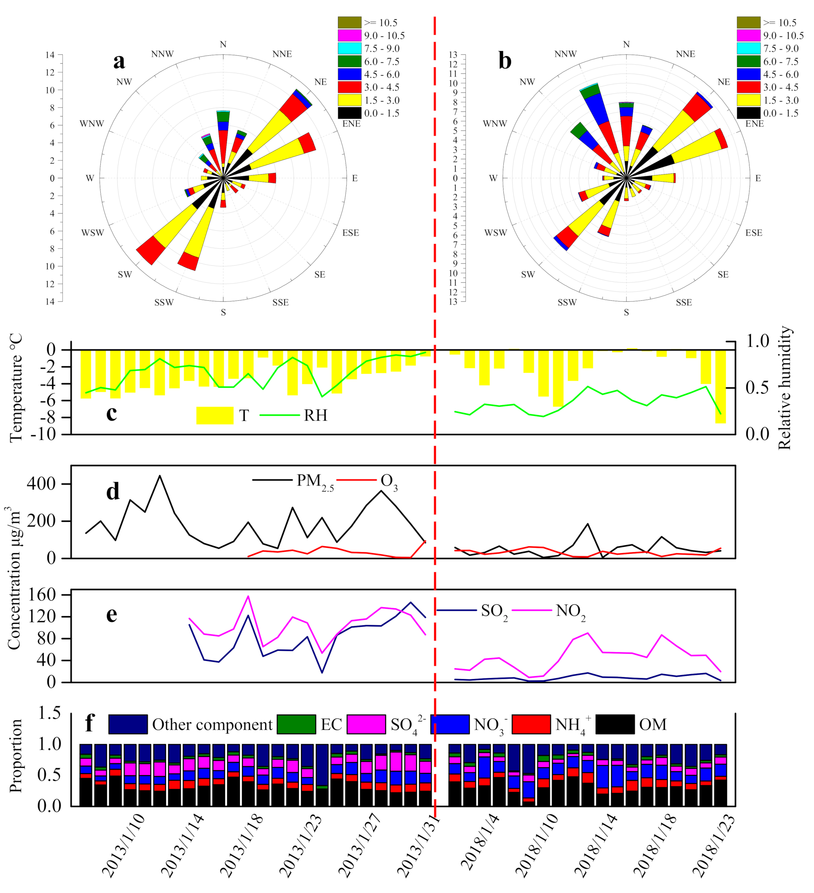
3.1. Characteristics of PM2.5 and O3

As presented in previous studies, severe pollution episodes occurred frequently in the North China Plain in the winter of 2013 [49,50]. In this study, daily samples were measured in January 2013 and 2018. The pollution variations were discussed on the basis of air pollutant concentrations and chemical components of PM2.5 (Tables S1 and S2 of the Supplementary Materials). Figure 1 shows the concentrations of PM2.5, SO2, and NO2 during the sampling periods. The average PM2.5 concentrations in January 2013 and 2018 were 184.7 ± 103.4μg/m3 (from 53.6 μg/m3 to 445.2 μg/m3) and 51.0 ± 41.5 μg/m3 (from 5.0 μg/m3 to 186.3 μg/m3), respectively (Figure 1d). It was noted that the PM2.5 concentration in 2013 far exceeded level 2 of the China National Air Quality Standard (75 μg/m3). A daily concentration higher than 150 μg/m3 represents a degree of heavy pollution accounting for more than 50%. SO2 and NO2 were the major precursors of PM2.5. Their average concentrations were 83.3 ± 35.1 μg/m3 and 104.3 ± 26.0 μg/m3 in 2013 and 8.8 ± 4.5 μg/m3 and 45.8 ± 22.9 μg/m3 in 2018, respectively (Figure 1e). Meteorological conditions were non-negligible drivers responsible for the formation of haze. Wind speed and relative humidity were important factors affecting the physical diffusion and chemical conversion of pollutants. The average wind speeds were 1.8 ± 1.1 m/s and 2.3 ± 1.4 m/s in 2013 and 2018, respectively (Table S3 of the Supplementary Materials). The frequency of southwest wind was higher in 2013 than in 2018 (Figure 1a,b). It is well known that the emission load in cities located to the south of Beijing is larger. Thus, the wind field in 2013 likely brought air pollutants into Beijing [31]. In addition, the significantly (p = 4.71 × 10⁻¹⁰) higher relative humidity in 2013 (60.6% ± 23.1%) compared with 2018 (32.1% ± 15.4%) (Figure 1c) could have provided adequate conditions for the secondary conversion of precursors including SO2 and NOx to generate SO42− and NO3. The poor air quality in winter was highly related to coal-fired activities, which led to a large number of primary particulates and SO2 emissions in the past decade. Owing to joint regional prevention and control, pollutant emissions in Beijing and its surrounding regions saw a great fall from 2013 to 2018. Coupled with the extremely favorable weather conditions, the air quality achieved remarkable improvement in the winter of 2018.
The chemical components of PM2.5 were analyzed and divided into six groups, including elemental carbon (EC), organic matter (OM; 1.6 × OC), SO42−, NO3, NH4+, and other components (Figure 1f). Results showed that the proportion of OM accounted for the highest proportion with 31.7% ± 8.2% and 31.4% ± 9.8% in the two periods. This demonstrated that, although emission control strategies contributed to the sharp decrease in PM2.5 concentration, OM was still a key reason for the occurrence of air pollution. The proportions of EC were less than 5%. NO3, SO42−, and NH4+ (defined as SNA) were generated mainly from the secondary conversion, contributing majorly to heavy pollution. It is worth noting that the total proportion of SNA during the two sampling periods was similar with values of 41.1% ± 12.3% and 41.1% ± 7.1% in 2013 and 2018, respectively. They were ranked in the order of SO42− > NO3 > NH4+ in 2013 and NO3 > NH4+ > SO42− in 2018. The correlation coefficient between cations and anions in the target sampling periods ranged from 0.88 to 0.95. This indicated that the combination of NH4+ with SO42− and NO3 was the major form of SNA. However, the ammonia-rich situation in Beijing is becoming more prominent according to ion equilibrium calculations [51]. It was mainly due to the strict control of sulfur-containing pollutants. On the other hand, reduction in NH3 emissions (livestock and fertilizer application) was not a key issue during the past few years. The sulfur oxidation ratio (SOR) and nitrogen oxidation ratio (NOR) are widely used to evaluate the conversion of SO2 and NOx. These values were 0.17 ± 0.10 and 0.14 ± 0.07 in 2013 and 0.25 ± 0.14 and 0.15 ± 0.10 in 2018, respectively. Positive correlations of SOR and SO42− with NOR and NO3 were observed with values larger than 0.5 during the study period. This indicated that the secondary conversion of precursors might have been a reason for high concentrations of SO42− and NO3. As mentioned above, the concentrations of SO2 and NO2 were significantly (SO2, p = 1.93 × 10⁻¹⁰; NO2, p = 4.9 × 10⁻⁸) lower in 2018 (8.8 ± 4.5 μg/m3 and 45.8 ± 22.9 μg/m3) compared to 2013 (83.3 ± 35.1 μg/m3 and 104.3 ± 26.0 μg/m3). However, the O3 concentration remained at a similar degree with values of 35.2 ± 24.2 μg/m3 and 32.1 ± 15.5 μg/m3. This demonstrated that the atmospheric oxidation capacity of the Beijing area was not weakened under the conditions of continuous and substantial emission reduction. On the other hand, the implementation of stricter control strategies for sulfur pollutants in Beijing compared to its surrounding regions might have caused Beijing to be affected more by their transmission.
O3 is an important indicator of atmospheric oxidation degree. It can promote the secondary conversion of SO2 and NOx through homogeneous and heterogeneous reactions to generate SO42− and NO3. Negative correlations were obtained between O3 and PM2.5 (−0.41 and −0.61), O3 and SO2 (−0.43 and −0.86), and O3 and NO2 (−0.70 and −0.91). Although O3 was not the primary air pollutant in the studied periods, it played an important role in the formation of PM2.5 pollution. Hence, for an effective improvement in PM2.5 pollution, coordinated control of O3 pollution is needed.

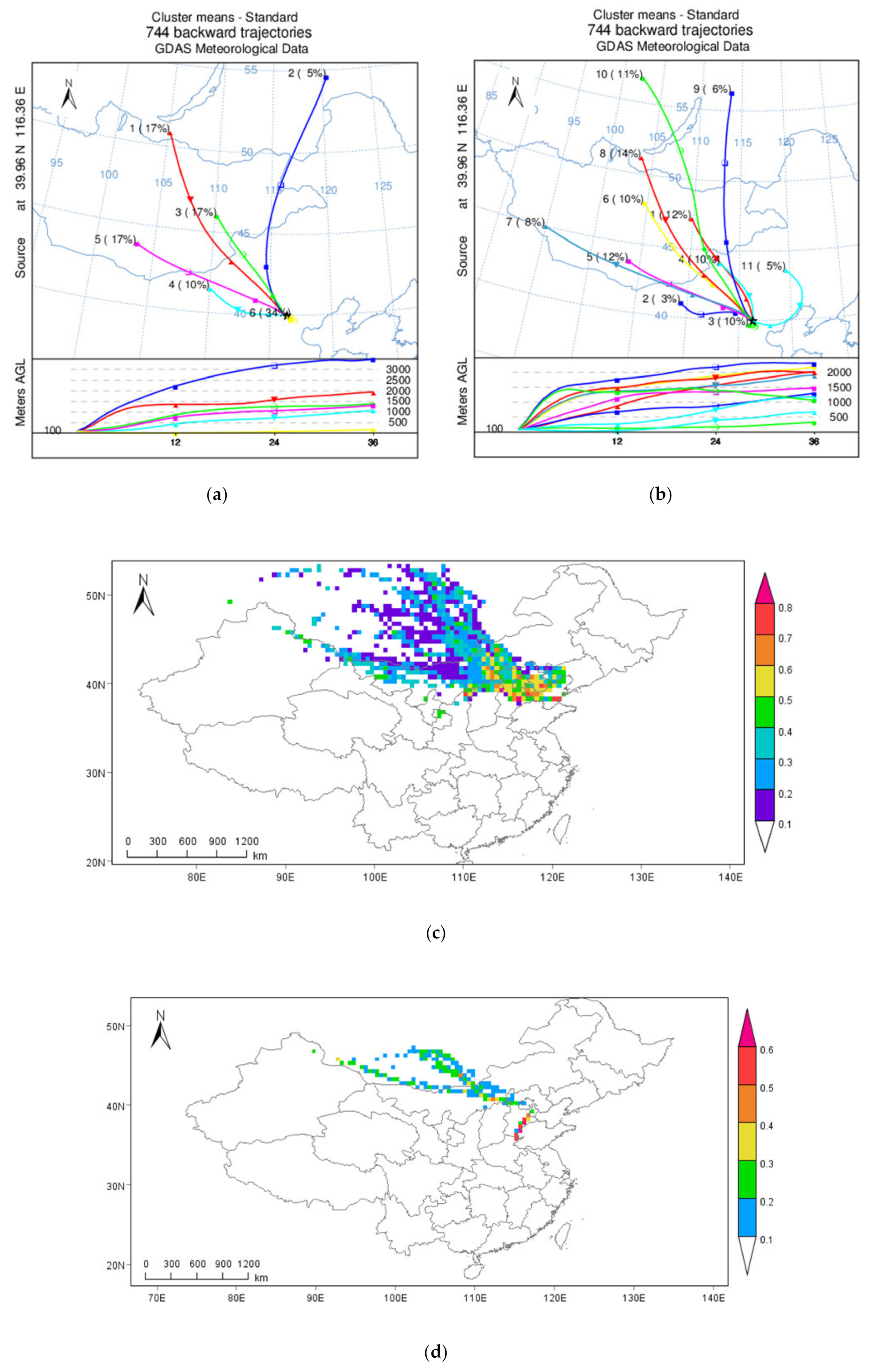
3.2. Potential Pollution Sources

The 36 h backward trajectory of air mass and the potential pollution sources of air mass in January 2013 and 2018 in Beijing are shown in Figure 2. The results presented similar characteristics, showing that air mass mainly came from the northwestern, western, and southern nearby regions during the two studied periods. In January 2013, for orientation, air mass from the northwestern region showed a lower PSCF value and higher height (above 1000 m), while air mass from the southern nearby region showed a higher PSCF value and lower height, typically transported from the surface layer. As for January 2018, the northwestern air mass also showed a lower PSCF value accompanied with a height of more than 1000 m, while air mass from the southern nearby region displayed similar characteristics to that in 2013. It is well known that cold air from the upper northwest usually leads to a marked improvement in Beijing’s air quality, while southern air mass is responsible for polluted days since the emission level of southern cities is much larger [52]. It is worth noting that the southern nearby air mass accounted for 34% and 10% of the total during the two periods. This demonstrated that the meteorological conditions in 2013 were more favorable for the formation of haze, consistent with the analysis of wind field. Overall, the higher PM2.5 concentration of Beijing was closely related to the local emission discharge, as well as the transport of external pollution sources from southern regions. The better air quality in January 2018 benefited from meteorological conditions that were more conducive to the diffusion of pollutants.

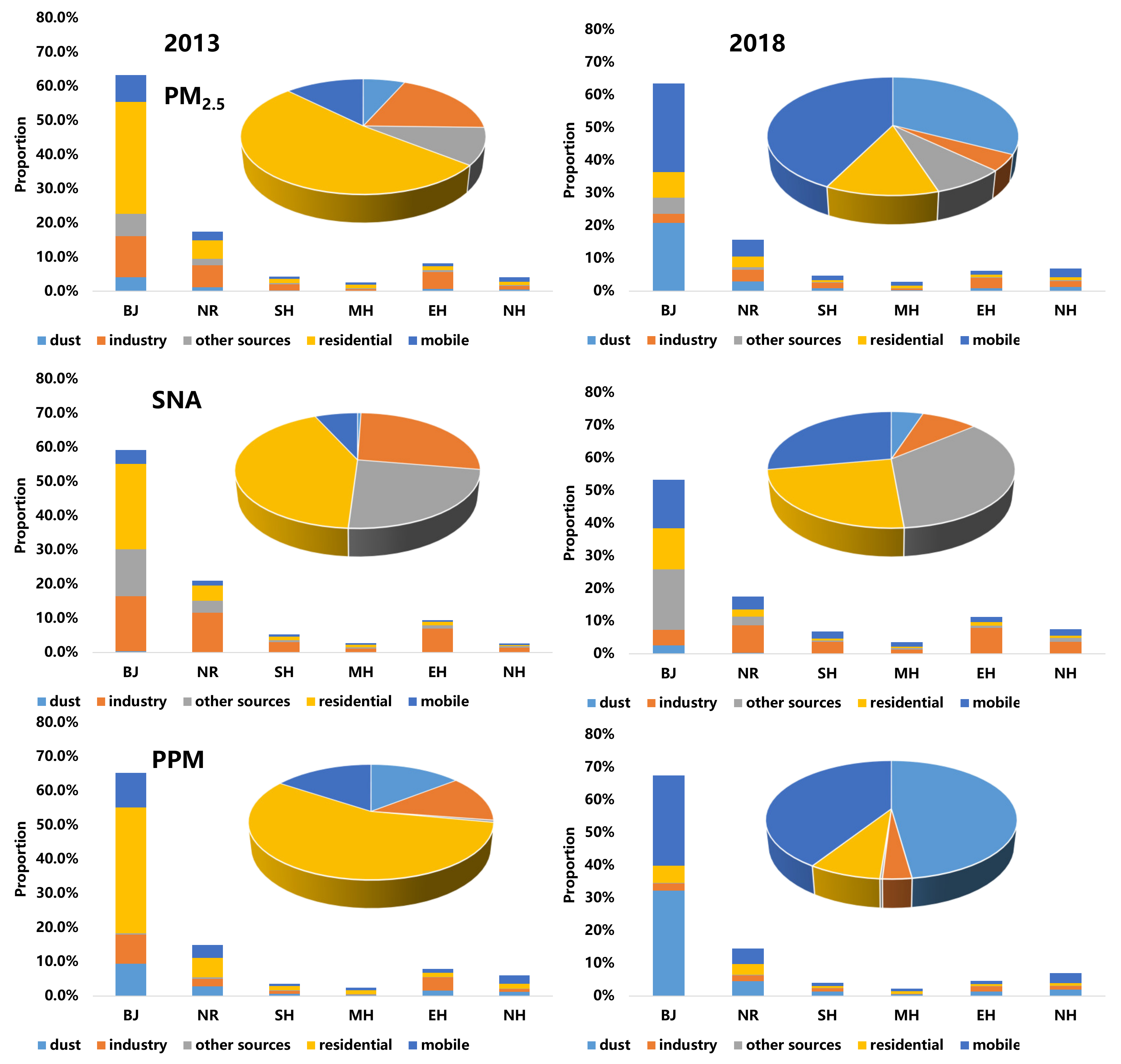
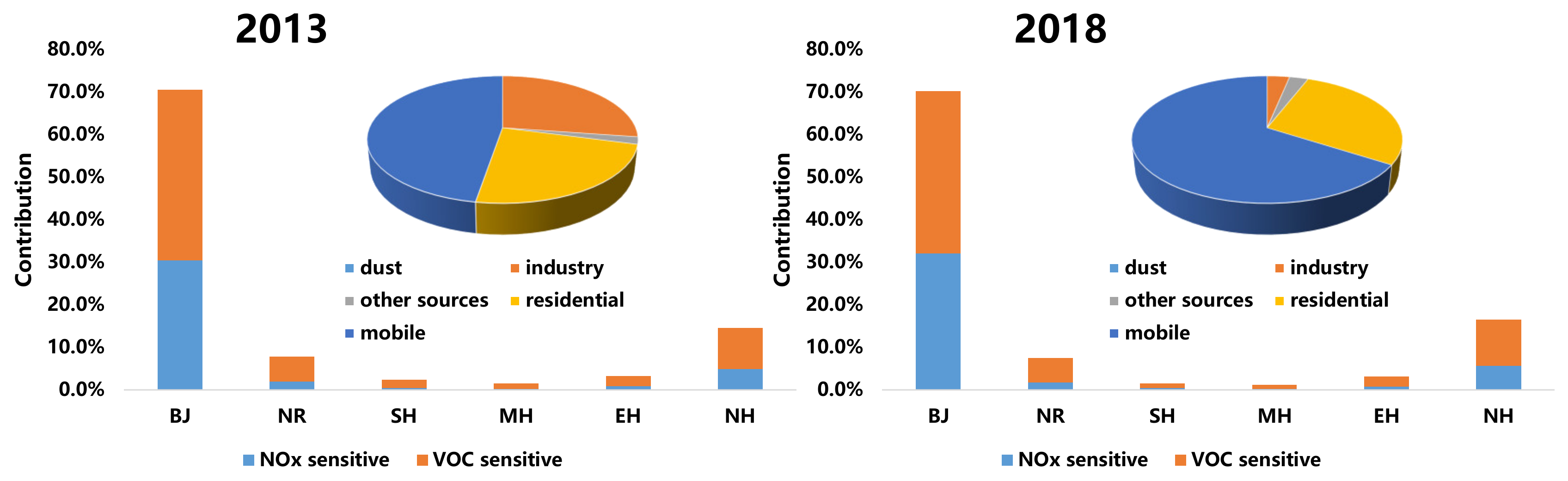
3.3. Source Apportionment of PM2.5 and O3

In order to guarantee a rapid and effective improvement in air quality for Beijing and its surrounding regions, strict control measurements have been implemented in the past decade. Thus, the contribution of various sources to atmospheric compound pollutants varied throughout the two study periods. Figure 3 shows the average contribution of the five major sources to PM2.5 and its major components, as well as O3. Local emissions contributed 63.3% and 63.5% to the total PM2.5 concentration during the two study periods. In the surrounding regions, they ranked in the order of NR > EH > SH > NH > MH in 2013 and NR > NH > EH > SH > MH in 2018. A larger contribution of NR was obtained in 2013 compared with that in 2018, while the contribution of the northern area (NH) in 2013 was much smaller. Since severe PM2.5 pollution was observed in January 2013, the poor air quality was closely related to the transport of air pollutants, especially from nearby cities located in the southern region. SNA was mainly converted from precursors including SO2, NOx, and NH3. The regional contribution was ranked in the order of NR > EH > SH > MH > NH in 2013 and NR > EH > NH > SH > MH in 2018. Primary particulate matter (PPM) was generally as a result of primary emissions. NR contributed most among the surrounding regions, followed by EH and NH in 2013, while NH and EH contributed most in 2018. It is worth noting that the regional emission contribution of SNA was larger than PPM during the two periods. This demonstrated that primary pollution was affected more by local and nearby emissions. However, SNA is more concentrated in fine particles and submicron particles, which are much more easily transported over longer distances.
From the perspective of various emissions, the residential and industrial sources were two dominant contributors to total PM2.5, SNA, and PPM in January 2013, accounting for 69.2%, 72.3%, and 64.1%, respectively. On the other hand, in 2018, mobile sources and dust contributed the most to total PM2.5 with proportions of 38.7% and 27.1%, and to PPM with proportions of 98.4% and 41.9%. As for SNA, the industry and mobile sources accounted for 29.2% and 25.8%. In terms of local emissions, residential sources were the predominant contributor to total PM2.5, SNA, and PPM with proportions of 51.8%, 42.3%, and 56.3% in January 2013, respectively. On the other hand, in 2018, they decreased to 12.2%, 23.5%, and 7.8%, with mobile sources and dust becoming much larger compared with 2013. It is well known that Beijing and its surrounding regions have tightened controls especially with regard to industrial and combustion sources since 2013 [31,51]. A policy titled “Interim Measures for Replacing and Reducing the Coal Consumption in Key Regions” claimed that the coal consumption of the Beijing–Tianjin–Hebei region decreased by 63 million from 2012 to 2017, and coal-fired boilers with a capacity of 35 tons or less were phased out in all urban areas, while those with a capacity of 10 tons or less were phased out in rural areas. In addition, BTH regions have continuously and vigorously promoted the policy of “coal to gas” and “coal to electricity”, which has achieved apparent results in terms of the reduction in coal consumption. Remarkable results have also been achieved in the treatment of thermal power plants. The BTH region has completed the transformation of ultra-low emissions and achieved full coverage of desulfurization, denitration, and dust removal facilities. Metallurgy, building materials, and chemical industries have also carried out different levels of governance. Thus, the contribution of industry and residential sources to PM2.5 and its components decreased from 2013 to 2018. As for the mobile sources, although the standards of vehicle emission have become stricter and the control over diesel vehicles has been strengthened, the number of vehicles in BTH regions is still on the rise year by year. The contribution of mobile sources to PM2.5 pollution has, thus, become more prominent.
Figure 4 presents the local emission contribution to O3, as well as the sensitive analysis related to NOx and VOC. Simulation results indicated that local emission sources contributed more than 70% to total O3 concentration in January 2013 and 2018. The industry contribution decreased, while the contribution of mobile sources increased from 2013 to 2018. This demonstrated that the variation in O3 pollution was closely related to the adjustment of energy structure. NOx and VOC were predominant precursors of O3. A nonlinear relationship was reported between the emission of precursors and the formation of O3. Due to the influence of meteorological conditions and emission amount, the ozone generation mechanism in a certain area was dynamic and could change. The reduction of a single pollutant could have led to the increase in ozone concentration. Results showed that around 60% of total O3 was generated related to VOC-sensitive areas. Moreover, with the reduction in NOx during the past decade, this feature did not show obvious changes. Therefore, in order to control ozone pollution more effectively, the control of VOC should be strengthened in the next stage.

3.4. Emission Reduction Effect on PM2.5 Pollution Improvement

In order to distinguish the effects of emission control measurements and the variations in meteorological conditions on the improvement in air pollution, four scenarios were measured as follows: (a) inventory coupled with meteorological conditions of 2013; (b) inventory coupled with meteorological conditions of 2018; (c) inventory based on 2013 coupled with meteorological conditions of 2018; (d) inventory based on 2018 coupled with meteorological conditions of 2013. The difference between (a) and (c) represented the effect of meteorological conditions on air pollution, while the difference between (a) and (d) represented the effect of a reduction in emissions on air pollution. Results showed that the emission control measurement contributed 41.0%, 36.1%, and 21.1% to the decrease in PM2.5, SO42−, and NO3 concentrations on a monthly average level. This showed that the emission reduction of pollution sources had a positive effect on the improvement in air quality. The better improvement of SO42− was due to the stricter control of coal burning from 2013 to 2018. On the contrary, the vehicle population, which was the major source of NOx emissions, increased continuously during the past decade. As mentioned in Section 3.1, the meteorological conditions in 2018 were more favorable for the diffusion and removal of air pollutants. The simulation results indicated that the change in meteorological conditions contributed more than the reduction in air pollutants, playing a more dominant role in the improvement in air quality. This demonstrated that the effect of pollutant emission reduction on air quality improvement was weakened under extremely adverse meteorological conditions.

4. Conclusions

In this study, the variation in the characteristics of PM2.5 and O3 in the winter of 2013 and 2018 was discussed on the basis of monitoring data and simulation technology. Two sampling projects were measured in January 2013 and 2018, and daily PM2.5 samples were collected, with chemical components including water-soluble ions, carbon components, and inorganic element analyzed. Monitoring results showed that OM accounted the most for total PM2.5 during the two study periods, which represents a key problem in the next stage of particulate control. Secondary inorganic ions were ranked in the order of SO42− > NO3 > NH4+ in 2013 and NO3 > NH4+ > SO42− in 2018. SOR and NOR both increased from 2013 to 2018. This demonstrated that the chemical composition changed with the implementation of strict control policies on various sources including coal, vehicles, and industrial emissions. The conversion degree of precursors might have been enhanced although their concentration dropped sharply. The 36 h backward trajectory of air mass and potential pollution source analysis were applied to qualitatively analyze the formation of pollution during the two studied periods. It was found that northwestern and southern nearby air mass were the two major input directions during both periods. The high concentration of PM2.5 was closely related to the air mass transport from the surface layer of the southern nearby region. In addition, more air mass came from the southern direction in 2013 than 2018. This demonstrated that the wind field of 2018 was more favorable for the diffusion of pollutants. A WRF-CAMx modeling system was established to evaluate various regions and source contributions to the concentration of PM2.5 and its major components in January 2013 and 2018. It was found that the contribution of industry sources to PM2.5 and O3 decreased while mobile sources increased from 2013 to 2018. Results of the O3 sensitivity analysis indicated that more control measurements should be taken with respect to VOCs since O3 concentration was affected more by VOCs during both periods. In addition, multiple scenarios were designed to recognize the emission reduction effect on the improvement in air quality. Results indicated that the reduction in various pollutant emissions played a positive role in the improvement in PM2.5 pollution. The changes in meteorological conditions played an even greater role in improving the air quality, as extremely adverse meteorological conditions could have weakened the effect of pollutant emission reduction on air quality improvement.

Supplementary Materials

The following are available online at https://www.mdpi.com/2073-4433/11/12/1324/s1, Table S1. Daily proportion of OM, NH4+, SO42−, NO3−, EC and other component (Ot) in PM2.5. Table S2. Daily concentration of PM2.5, SO2, NO2 and O3. Table S3. Daily temperature (T) and relative humidity (RH) during study period.

Author Contributions

Y.Z., X.W. and S.C. designed the simulation, collection and analysis of the data; Y.Z. and X.W. wrote the paper; S.C. and X.W. reviewed and edited the paper. All authors have read and agreed to the published version of the manuscript.

Funding

This research was funded by the National Natural Science Foundation of China (No. 51638001), the National Key R&D Program of China (2018YFC0213206), the Beijing Municipal Commission of Science and Technology (Z181100005418017), the China Postdoctoral Science Foundation (2019M660382) and Beijing Postdoctoral Research Foundation.

Conflicts of Interest

The authors declare no conflict of interest

References

  1. Wu, W.; Zhang, M.; Ding, Y. Exploring the effect of economic and environment factors on PM2.5 concentration: A case study of the Beijing-Tianjin-Hebei region. J. Environ. Manag. 2020, 268, 110703. [Google Scholar] [CrossRef] [PubMed]
  2. Yang, G.; Huang, J.; Li, X. Mining sequential patterns of PM2.5 pollution in three zones in China. J. Clean. Prod. 2018, 170, 388–398. [Google Scholar] [CrossRef]
  3. Gui, K.; Che, H.; Wang, Y.; Wang, H.; Zhang, L.; Zhao, H.; Zheng, Y.; Sun, T.; Zhang, X. Satellite-derived PM2.5 concentration trends over Eastern China from 1998 to 2016: Relationships to emissions and meteorological parameters. Environ. Pollut. 2019, 247, 1125–1133. [Google Scholar] [CrossRef] [PubMed]
  4. Wu, X.; Xin, J.; Zhang, X.; Klaus, S.; Wang, Y.; Wang, L.; Wen, T.; Liu, Z.; Si, R.; Liu, G.; et al. A new approach of the normalization relationship between PM2.5 and visibility and the theoretical threshold, a case in north China. Atmos. Res. 2020, 245, 105054. [Google Scholar] [CrossRef]
  5. Zheng, G.; Duan, F.; Su, H.; Ma, Y.; Cheng, Y.; Zhang, B.; Zhang, Q.; Huang, T.; Kimoto, T.; Chang, D.; et al. Exploring the severe winter haze in Beijing: The impact of synoptic weather, regional transport and heterogeneous reactions. Atmos. Chem. Phys. 2015, 15, 2969–2983. [Google Scholar] [CrossRef] [Green Version]
  6. Tetsuya, T.; Shunsuke, M. Health-related and non-health-related effects of PM2.5 on life satisfaction: Evidence from India, China and Japan. Econ. Anal. Policy 2020, 67, 114–123. [Google Scholar]
  7. Chen, H.; Li, L.; Lei, Y.; Wu, S.; Yan, D.; Dong, Z. Public health effect and its economics loss of PM2.5 pollution from coal consumption in China. Sci. Total Environ. 2020, 732, 138973. [Google Scholar] [CrossRef]
  8. Westervelt, D.; Horowitz, L.; Naik, V.; Tai, A.; Fiore, A.; Mauzerall, D. Quantifying PM2.5—Meteorology Sensitivities in a Global Climate Model. Atmos. Environ. 2016, 142, 43–56. [Google Scholar] [CrossRef]
  9. Gao, L.; Wang, T.; Ren, X.; Zhuang, B.; Li, S.; Yao, R.; Yang, X. Impact of atmospheric quasi-biweekly oscillation on the persistent heavy PM2.5 pollution over Beijing-Tianjin-Hebei region, China during winter. Atmos. Res. 2020, 242, 105017. [Google Scholar] [CrossRef]
  10. Baker, K.; Foley, K. A nonlinear regression model estimating single source concentrations of primary and secondarily formed PM2.5. Atmos. Environ. 2011, 45, 3758–3767. [Google Scholar] [CrossRef]
  11. Wang, Y.; Liu, Z.; Lu, G.; Gong, Y.; Elly, Y.; Li, H.; Yi, X.; Yang, L.; Feng, J.; Ivey, C.; et al. Development and Evaluation of a Scheme System of Joint Prevention and Control of PM2.5 Pollution in the Yangtze River Delta Region, China. J. Clean. Prod. 2020, 275, 122756. [Google Scholar] [CrossRef]
  12. Cai, S.; Wang, Y.; Zhao, B.; Wang, S.; Chang, X.; Hao, J. The impact of the “Air Pollution Prevention and Control Action Plan” on PM2.5 concentrations in Jing-Jin-Ji region during 2012–2020. Sci. Total Environ. 2017, 580, 197–209. [Google Scholar] [CrossRef] [PubMed]
  13. Huang, X.; Tang, G.; Zhang, J.; Liu, B.; Liu, C.; Zhang, J.; Cong, L.; Cheng, M.; Yan, G.; Gao, W.; et al. Characteristics of PM2.5 pollution in Beijing after the improvement of air quality. J. Environ. Sci. 100, 1–10. [CrossRef] [PubMed]
  14. Yang, K.; Li, Q.; Yuan, M.; Guo, M.; Wang, Y.; Li, S.; Tian, C.; Tang, J.; Sun, J.; Li, J.; et al. Temporal variations and potential sources of organophosphate esters in PM2.5 in Xinxiang, North China. Chemosphere 2018, 215, 500–506. [Google Scholar] [CrossRef]
  15. Zong, Z.; Wang, X.; Tian, C.; Chen, Y.; Fu, S.; Qu, L.; Ji, L.; Li, J.; Zhang, G. PMF and PSCF based source apportionment of PM2.5 at a regional background site in North China. Atmos. Res. 2018, 203, 207–215. [Google Scholar] [CrossRef] [Green Version]
  16. Zhao, J.; Ma, X.; Wu, S.; Sha, T. Dust emission and transport in Northwest China: WRF-Chem simulation and comparisons with multi-sensor observations. Atmos. Res. 2020, 241, 104978. [Google Scholar] [CrossRef]
  17. Hong, J.; Mao, F.; Min, Q.; Pan, Z.; Wang, W.; Zhang, T.; Gong, W. Improved PM2.5 predictions of WRF-Chem via the integration of Himawari-8 satellite data and ground observations. Environ. Pollut. 2020, 263, 114451. [Google Scholar] [CrossRef]
  18. Pirovano, G.; Colombi, C.; Balzarini, A.; Riva, G.; Gianelle, V.; Lonati, G. PM2.5 source apportionment in Lombardy (Italy): Comparison of receptor and chemistry-transport modelling results. Atmos. Environ. 2015, 106, 56–70. [Google Scholar] [CrossRef]
  19. Pepe, N.; Pirovano, G.; Balzarini, A.; Toppetti, A.; Riva, G.; Amato, F.; Lonati, G. Enhanced CAMx source apportionment analysis at an urban receptor in Milan based on source categories and emission regions. Atmos. Environ. 2019, 2, 100020. [Google Scholar] [CrossRef]
  20. Zhang, Y.; Li, X.; Nie, T.; Qi, J.; Chen, J.; Wu, Q. Source apportionment of PM2.5 pollution in the central six districts of Beijing, China. J. Clean. Prod. 2018, 174, 661–669. [Google Scholar] [CrossRef]
  21. Lang, J.; Zhang, Y.; Zhou, Y.; Cheng, S.; Chen, D.; Guo, X.; Chen, S.; Li, X.; Xing, X.; Wang, H. Trends of PM2.5 and Chemical Composition in Beijing, 2000–2015. Aerosol Air Qual. Res. 2017, 17, 412–425. [Google Scholar] [CrossRef]
  22. Lang, J.; Cheng, S.; Li, J.; Chen, D.; Zhou, Y.; Wei, X.; Han, L.; Wang, H. A monitoring and modeling study to investigate regional transport and characteristics of PM2.5 pollution. Aerosol Air Qual. Res. 2013, 13, 943–956. [Google Scholar] [CrossRef] [Green Version]
  23. Yu, S.; Liu, W.; Xu, Y.; Yi, L.; Zhou, M.; Tao, S.; Liu, W. Characteristics and oxidative potential of atmospheric PM2.5 in Beijing: Source apportionment and seasonal variation. Sci. Total Environ. 2019, 650, 277–287. [Google Scholar] [CrossRef] [PubMed]
  24. Wu, X.; Chen, C.; Vu, T.; Liu, D.; Baldo, C.; Shen, X.; Zhang, Q.; Cen, K.; Zheng, M.; He, K.; et al. Source apportionment of fine organic carbon (OC) using receptor modelling at a rural site of Beijing: Insight into seasonal and diurnal variation of source contributions. Environ. Pollut. 2020, 266, 115078. [Google Scholar] [CrossRef]
  25. Hao, Y.; Meng, X.; Yu, X.; Lei, M.; Li, W.; Yang, W.; Shi, F.; Xie, S. Quantification of primary and secondary sources to PM2.5 using an improved source regional apportionment method in an industrial city, China. Sci. Total Environ. 2020, 706, 135715. [Google Scholar] [CrossRef]
  26. Wang, T.; Du, Z.; Tan, T.; Xu, N.; Hu, M.; Hu, J.; Guo, S. Measurement of Aerosol Optical Properties and Their Potential Source Origin in Urban Beijing from 2013–2017. Atmos. Environ. 2019, 206, 293–302. [Google Scholar] [CrossRef]
  27. Jiang, C.; Wang, H.; Zhao, T.; Li, T.; Che, H. Modeling study of PM2.5 pollutant transport across cities in China’s Jing-Jin-Ji region during a severe haze episode in December 2013. Atmos. Chem. Phys. 2015, 15, 5803–5814. [Google Scholar] [CrossRef] [Green Version]
  28. Chang, X.; Wang, S.; Zhao, B.; Xing, J.; Liu, X.; Wei, L.; Song, Y.; Wu, W.; Cai, S.; Zheng, H.; et al. Contributions of inter-city and regional transport to PM2.5 concentrations in the Beijing-Tianjin-Hebei region and its implications on regional joint air pollution control. Sci. Total Environ. 2019, 660, 1191–1200. [Google Scholar] [CrossRef]
  29. Sun, X.; Cheng, S.; Lang, J.; Ren, Z.; Sun, C. Development of emissions inventory and identification of sources for priority control in the middle reaches of Yangtze River Urban Agglomerations. Sci. Total Environ. 2018, 625, 155–167. [Google Scholar] [CrossRef]
  30. Jiang, L.; He, S.; Zhou, H. Spatio-temporal characteristics and convergence trends of PM2.5 pollution: A case study of cities of air pollution transmission channel in Beijing-Tianjin-Hebei region, China. J. Clean. Prod. 2020, 256, 120631. [Google Scholar] [CrossRef]
  31. Wang, X.; Wei, W.; Cheng, S.; Li, J.; Zhang, H.; Lv, Z. Characteristics and classification of PM2.5 pollution episodes in Beijing from 2013 to 2015. Sci. Total Environ. 2018, 612, 170–179. [Google Scholar] [CrossRef] [PubMed]
  32. Wang, H.; Zhao, L. A joint prevention and control mechanism for air pollution in the Beijing-Tianjin-Hebei region in china based on long-term and massive data mining of pollutant concentration. Atmos. Environ. 2018, 174, 25–42. [Google Scholar] [CrossRef]
  33. Chen, Z.; Chen, D.; Kwan, M.; Chen, B.; Gao, B.; Zhuang, Y.; Li, R.; Xu, B. The control of anthropogenic emissions contributed to 80% of the decrease in PM2.5 concentrations in Beijing from 2013 to 2017. Atmos. Chem. Phys. 2019, 19, 13519–13533. [Google Scholar] [CrossRef] [Green Version]
  34. Hu, W.; Zhao, T.; Bai, Y.; Shen, L.; Sun, X.; Gu, Y. Contribution of regional PM2.5 transport to air pollution enhanced by sub-basin topography: A modeling case over central China. Atmosphere 2020, 11, 1258. [Google Scholar] [CrossRef]
  35. Su, L.; Yuan, Z.; Fung, J.; Lau, A. A comparison of HYSPLIT backward trajectories generated from two GDAS datasets. Sci. Total Environ. 2015, 506, 527–537. [Google Scholar] [CrossRef]
  36. Chen, C.; Sasa, K.; Ohsawa, T.; Kashiwagi, W.; Prpic-Orsic, J.; Mizojiri, T. Comparative assessment of NCEP and ECMWF global datasets and numerical approaches on rough sea ship navigation based on numerical simulation and shipboard measurements. Appl. Ocean Res. 2020, 101, 102219. [Google Scholar] [CrossRef]
  37. Shi, X.; Girid, L.; Long, R.; DeKett, R.; Philippe, J.; Burke, T. A comparison of LiDAR-based DEMs and USGS-sourced DEMs in terrain analysis for knowledge-based digital soil mapping. Geoderma 2012, 170, 217–226. [Google Scholar] [CrossRef]
  38. Zhou, Y.; Cheng, S.; Li, J.; Lang, J.; Li, L.; Chen, D. A new statistical modeling and optimization framework for establishing high-resolution PM10 emission inventory-II. Integrated air quality simulation and optimization for performance improvement. Atmos. Environ. 2012, 60, 623–631. [Google Scholar] [CrossRef]
  39. Lang, J.; Tian, J.; Zhou, Y.; Li, K.; Chen, D.; Huang, Q.; Xing, X.; Zhang, Y.; Cheng, S. A high temporal-spatial resolution air pollutant emission inventory for agricultural machinery in China. J. Clean. Prod. 2018, 183, 1110–1121. [Google Scholar] [CrossRef]
  40. Zhang, T.; Zang, L.; Wan, Y.; Wang, W.; Zhang, Y. Ground-level PM2.5 estimation over urban agglomerations in China with high spatiotemporal resolution based on Himawari-8. Sci. Total Environ. 2019, 676, 535–544. [Google Scholar] [CrossRef]
  41. Chen, D.; Liu, X.; Lang, J.; Zhou, Y.; Wei, L.; Wang, X.; Guo, X. Estimating the contribution of regional transport to PM2.5 air pollution in a rural area on the North China Plain. Sci. Total Environ. 2017, 583, 280–291. [Google Scholar] [CrossRef] [PubMed]
  42. Zhang, Y.; Lang, J.; Cheng, S.; Li, S.; Zhou, Y.; Chen, D.; Zhang, H.; Wang, H. Chemical composition and source of PM1 and PM2.5 in Beijing in autumn. Sci. Total Environ. 2018, 630, 72–82. [Google Scholar] [CrossRef] [PubMed]
  43. Zhang, H.; Cheng, S.; Wang, X.; Yao, S.; Zhu, F. Continuous monitoring, compositions analysis and the implication of regional transport for submicron and fine aerosols in Beijing, China. Atmos. Environ. 2018, 195, 30–45. [Google Scholar] [CrossRef]
  44. Zhang, H.; Cheng, S.; Yao, S.; Wang, X.; Wang, C. Insights into the temporal and spatial characteristics of PM2.5 transport flux across the district, city and region in the North China Plain. Atmos. Environ. 2019, 218, 117010. [Google Scholar] [CrossRef]
  45. Wang, X.; Wei, W.; Cheng, S.; Zhang, H.; Yao, S. Source estimation of SO42− and NO3 based on monitoring-modeling approach during winter and summer seasons in Beijing and Tangshan, China. Atmos. Environ. 2019, 214, 116849. [Google Scholar] [CrossRef]
  46. Zhou, Y.; Zi, T.; Lang, J.; Huang, D.; Wei, P.; Chen, D.; Cheng, S. Impact of rural residential coal combustion on air pollution in Shandong, China. Chemosphere 2020, 260, 127517. [Google Scholar] [CrossRef]
  47. Chen, D.; Liu, Z.; Fast, J.; Ban, J. Simulations of sulfate-nitrate-ammonium (SNA) aerosols during the extreme haze events over northern China in October 2014. Atmos. Chem. Phys. 2016, 16, 10707–10724. [Google Scholar] [CrossRef] [Green Version]
  48. Wang, X.; Wei, W.; Cheng, S.; Zhang, C.; Duan, W. A monitoring-modeling approach to SO42− and NO3 secondary conversion ratio estimation during haze periods in Beijing, China. J. Environ. Sci. 2018, 78, 293–302. [Google Scholar] [CrossRef]
  49. Wang, H.; Xu, J.; Zhang, M.; Yang, Y.; Shen, X.; Wang, Y.; Chen, D.; Guo, J. A study of the meteorological causes of a prolonged and severe haze episode in January 2013 over central-eastern China. Atmos. Environ. 2014, 98, 146–157. [Google Scholar] [CrossRef]
  50. Zhang, J.; Sun, Y.; Liu, Z.; Ji, D.; Hu, B.; Liu, Q.; Wang, Y. Characterization of submicron aerosols during a month of serious pollution in Beijing, 2013. Atmos. Chem. Phys. 2014, 14, 2887–2903. [Google Scholar] [CrossRef] [Green Version]
  51. Yang, X.; Cheng, S.; Li, J.; Lang, J.; Wang, G. Characteristics of chemical composition in PM2.5 in Beijing before, during, and after a Large-Scale International Event. Aerosol Air Qual. Res. 2017, 17, 896–907. [Google Scholar] [CrossRef]
  52. Zhao, N.; Wang, G.; Li, G.; Lang, J.; Zhang, H. Air pollution episodes during the COVID-19 outbreak in the Beijing-Tianjin-Hebei region of China: An insight into the transport pathways and source distribution. Environ. Pollut. 2020, 267, 115617. [Google Scholar] [CrossRef] [PubMed]
Figure 1. (a) Wind rose diagram for January 2013; (b) wind rose diagram for January 2018; (c) daily temperature (T) and relative humidity (RH); (d) daily concentrations of PM2.5 and O3; (e) daily concentrations of NO2 and SO2; (f) daily chemical composition of PM2.5.
Atmosphere 11 01324 g001
Figure 2. Backward trajectory and potential source analysis. (a) Backward trajectory analysis in January 2013; (b) backward trajectory analysis in January 2018; (c) potential source analysis in January 2013; (d) potential source analysis in January 2018.
Atmosphere 11 01324 g002
Figure 3. Source apportionment of PM2.5 and its major components in January 2013 and 2018. Column charts representing the contribution of Beijing–Tianjin–Hebei (BTH) sources to Beijing; pie charts representing the local emission contribution.
Atmosphere 11 01324 g003
Figure 4. Source apportionment of O3 in January 2013 and 2018. Column charts representing the contribution of O3 related to NOx-sensitive and volatile organic compounds (VOC)-sensitive areas; pie charts representing the local emission contribution.
Atmosphere 11 01324 g004
Table 1. Verification of meteorology and air quality simulation effects. NMB, standardized average deviation; COR, correlation coefficient.
Time PeriodIndicatorsNMBCOR
2013PM2.5 concentration−8.7%0.69
Temperature−1.3%0.68
Wind speed22.2%0.46
2018PM2.5 concentration4.5%0.72
Temperature−0.7%0.88
Wind speed34.8%0.57
Publisher’s Note: MDPI stays neutral with regard to jurisdictional claims in published maps and institutional affiliations.

