Mobile Observation of Air Temperature and Humidity Distributions under Summer Sea Breezes in the Central Area of Osaka City

Abstract

Thermal environment of urban areas in the summertime has become harmful to human health due to global warming and the urban heat island (UHI) effect. Mobile observations enable us to obtain the distribution of air temperature at microscale, such as urban blocks, which cannot be captured by the coarse network of meteorological sites. A series of mobile measurements was executed in the central area of Osaka City in Japan, around the Nakanoshima district which lies between two rivers, to investigate the air temperature and humidity distributions in a built-up area under sea breeze conditions. Upper wind and surface temperature of the rivers were also observed using pilot balloons and infrared thermography camera, respectively. The mean air temperature in Nakanoshima was generally lower than that of the surrounding area. Urban geometries such as building density and building height seem to affect the mean air temperature by changing the ventilation efficiency. Humidity was inversely correlated with air temperature distribution but was higher at the confluence of rivers and green parks. The depth of the sea breeze layer was found to be about 1 km. Sea breezes close to the ground surface penetrated the city along the rivers, sandwiching the Nakanoshima district. During the daytime, the surface temperatures of the rivers were lower than the air temperature observed at the nearest stationary observation point, and the difference reached approximately 2 °C.

1. Introduction

The most notable feature of the urban heat island (UHI) effect is an increase in nocturnal temperature (e.g., Oke, 1987 [1]). In Japan, the mitigation of high diurnal temperatures in midsummer has become an important issue because the extremely high temperatures not only lead to excessive power consumption [2] by air conditioning units but increase the incidence of heat stroke [3,4,5]. Fujibe (2013) [6] showed, from an analysis based on vital statistics data for Japan between 1909 and 2011, that there is a positive correlation between summertime temperature (averaged for July and August) and heat-related mortality.

Since the thermal environment of urban areas in the summertime is becoming harmful to human health due to the UHI effects in addition to global warming [7,8,9], it is becoming increasingly important to pay attention to diurnal temperatures. In 2007, the Japan Meteorological Agency (JMA) defined a new statistical index on air temperature, “extremely hot day” (EHD) (daily maximum temperature ≥35 °C), in addition to previously defined indices of “hot day” (daily maximum temperature ≥30 °C) and “hot night” (daily minimum temperature ≥25 °C). The JMA issues “extreme high-temperature forecasts” when the predicted daily maximum temperature exceeds the EHD criteria. In order to prevent heat stroke, the Ministry of the Environment publishes on its website the current and forecast values of the wet bulb globe temperature (WBGT) [10] at the meteorological observation points of Automated Meteorological Data Acquisition System (AMeDAS) which is operated by JMA.

Osaka is the most populous metropolitan area in western Japan and is well known for its severe summertime thermal environment [11]. As of July 2019, the residential populations in Osaka Prefecture are 8.82 million. In Osaka Prefecture, more than 3500 people have been transported by ambulance for heat stroke every summer (May–September) since 2015; in 2018 and 2019, the number was 7138 and 5182, respectively [12]. The local government of Osaka City has used the “ventilation path” (in Japanese, Kaze-no-Michi) concept to create a future urban plan for the area [13] that will mitigate its severe summertime thermal environment by utilizing the cooling potential of the sea breezes that come from Osaka Bay.

In the areas that sea breezes penetrate, the air temperature distribution near the ground can be used to evaluate their cooling effect. However, the thermal environment near the ground is strongly affected by surrounding features such as buildings, roads, rivers, and parks. Especially in urban areas, where buildings are numerous, the urban canopy significantly affects the heat budget at the ground surface. The ventilation efficiency of a city block will strongly depend on its geometry [14,15,16] because mean wind speed is weakened and/or intensified by drag forces and building-induced eddies. The cooling effect of a sea breeze may differ in magnitude even within a small area. The air temperature distribution will therefore show complex patterns. Mobile observations enable us to obtain such a microscale distribution of local air temperature, which cannot be captured by the coarse network of meteorological sites.

Mobile measurement of air temperature distribution in an urban area has been carried out by various research groups, including universities, local governments, and citizen groups. Automobiles have often been used to cover an objective area when the area was relatively large. Nabeshima et al. (2006) [17] and Mizuno et al. (2009) [18] used an automobile to make mobile observations on the Osaka plain. Sahashi (1983) [19] evaluated the various errors in air temperature measurements obtained using automobiles and made some suggestions to minimize the incidence of observational errors. Some research groups targeting relatively small areas have used bicycles for mobile observation [20,21,22]. Since bicycles can go through narrow paths which automobiles cannot access (e.g., back streets, narrow bridges, and pathways in green parks), they can capture a more detailed pattern of air temperature distribution. Additionally, the air temperatures measured during a mobile observation using a car can be affected by the heat radiated from the hoods, roofs, and the tailpipes of the car itself and other passing cars. The use of bicycles rather than cars circumvents this problem. Mobile observation with bicycles is therefore effective for detailed research; however, the target area of such research is often limited to a linear path or a relatively small area. There are few studies involving a large number of observers on bicycles covering different areas simultaneously because a large-scale observation campaign requires a lot of staff and equipment.

In this study, we made a detailed investigation of mean temperature and humidity distributions in urban blocks in mid-summer in Nakanoshima district and the surrounding area, a central office area in Osaka City, from dense observations obtained using bicycles. The objective area was subdivided into 13 areas (only on the first day of the observation, it was divided into eight areas) and mobile observation was executed simultaneously in every area. We also conducted an observation of the upper winds and the surface temperatures of the rivers sandwiching Nakanoshima district. The relationship between building density and the cooling effect of the sea breezes was discussed.

2. Methods

2.1. Objective Area

Figure 1a shows the location of Osaka and our study area. Since Osaka plain is bordered by mountains to the north, the east, and the south, the westerly sea breezes coming from Osaka Bay in the daytime are expected to mitigate high temperature in the plain. Nakanoshima, which means “a river island” in Japanese, is located at the center of Osaka’s urban area and lies between the Dojima River and the Tosabori River to the north and the south, respectively (Figure 1b). The west side in the Nakanoshima district is occupied by large high-rise buildings, and there is a small green park on the district’s eastern edge. Outer sides of the Nakanoshima district are densely built-up areas comprised of mid-rise office buildings. The study area is fairly flat and lies at an altitude between 0 and 3 m above sea level.

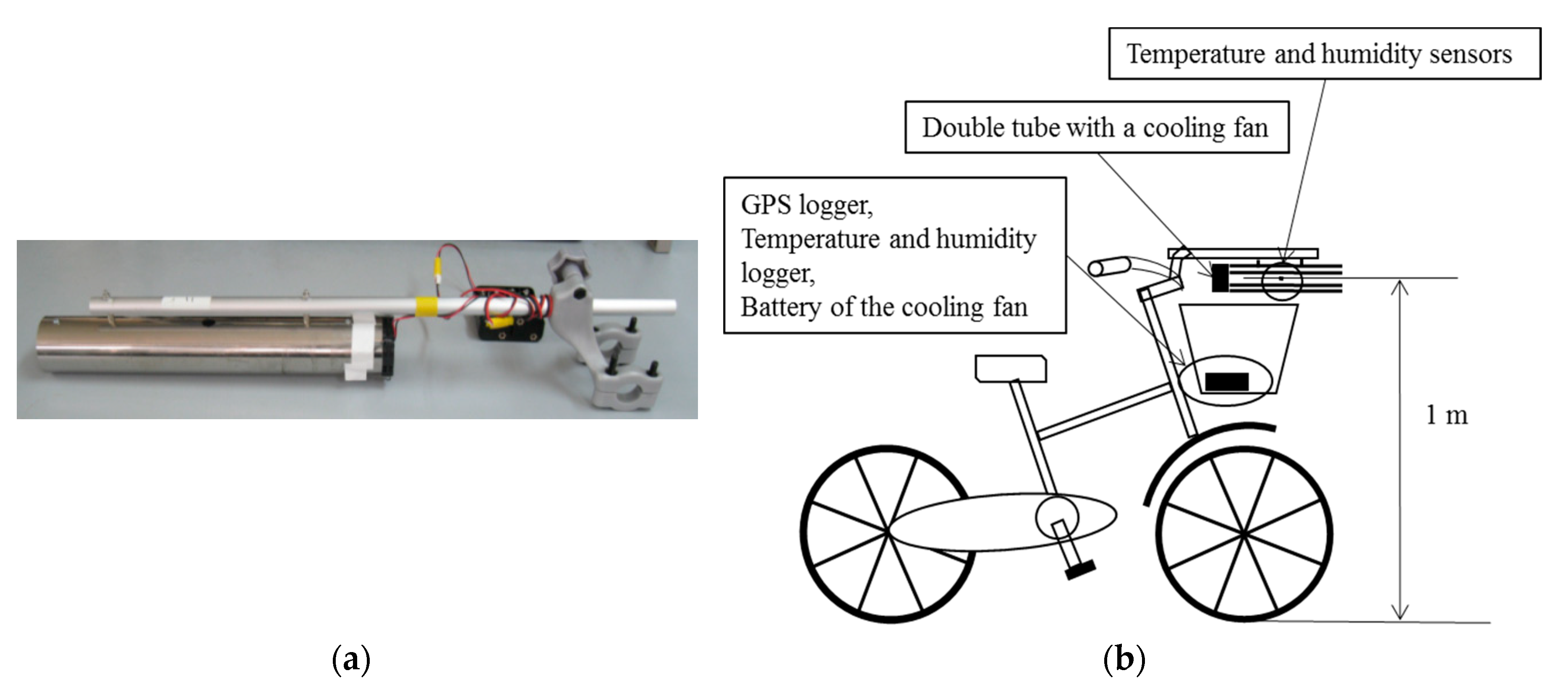
2.2. Mobile and Stationary Observations

Table 1. Outline and instruments of mobile observation.

Date	1 July, 28 July, 31 August 2010 (3 days)
Start Time	0900, 1100, 1400, 1600, 1800, 2000 LST (1 July and 31 August 2010) 0900, 1100. 1400, 1600, 1800 LST (28 July 2010)
Duration	30–40 min/run
Instruments	Temperature-only; RTR-52A (T&D Co.) Thermistor type, Accuracy: ±0.3 °C Temperature/Relative humidity; RTR-53A (T&D Co.) Thermistor/Polymer type, Accuracy: ±0.3 °C/±5% Latitude and Longitude; eTrex H (Garmin Co.) GPS Accuracy: <10 m r.m.s.
Record Interval	1 s

shows the outline and the instruments of the mobile observations. Figure 1b shows the observation area (enclosed in a white line), which is approximately 3.5 km E-W and 1.5 km N-S. The area was divided into 13 subareas (28 July and 31 August) (Figure 1c). However, on 1 July, due to equipment availability, the target area was divided into 8 subareas. In this case, subareas 2 and 3, 4 and 5, 10 and 11 were merged, and subareas 6 and 13 were excluded. The mobile observations were executed in all subareas simultaneously by travelling around them on bicycles. One bicycle was assigned to each area. To avoid the heat from direct solar radiation, we set a thermometer sensor (coupled with a hygrometer sensor in several cases) within a double tube made of stainless steel (Figure 2a). Steel tube has high solar reflectivity and low heat capacity, which are desirable properties to prevent the sensor from radiation heating. The double tubes were 300 mm in length. The diameter of the outer/inner tube used for the thermohygrometer coupled sensor was 50 mm/30 mm, and it was equipped with a motor fan to facilitate ventilation. The diameter of the double tube used for the thermo-only sensor was 45 mm/25 mm, and it was ventilated naturally (without a fan). The thermo-only sensors were used in subarea 1, 4, and 5 on 1 July (case of 8 subareas) and in subarea 5, 6, and 13 on 28 July and 31 August (case of 13 subareas). The thermohygrometer coupled sensors were used in the other subareas. The measurements were taken 1 m above the ground level (AGL) (Figure 2b).

On the days of the mobile observations, the temperature, humidity, wind, and short- and longwave radiation were measured continuously between 0900 and 2100 LST (see

Table 2. Outline and instruments of stationary observation at P2.

Date	1 July, 28 July, 31 August 2010 (3 days)
Time	0900-2100 LST
Height	1.5 m AGL
Instruments	Temperature/Relative humidity; HMT100 (Visala Co.) Pt/Polymer type in a double tube with a ventilation fan Accuracy: ±0.3 °C at 30 °C/±1.7% RH Wind; USA-1 (EKO Co.) Ultrasonic type, Accuracy: ±0.01 m/s Short- and Long-wave radiations; CNR1-10 (Field pro Co.) Accuracy: daily total ±10%
Record Interval	60 s

) at point P2 shown in Figure 1b in order to understand the meteorological conditions around the objective area. Additionally, pilot balloon observations of the upper winds (~2000 m AGL) were made at P2 intermittently. These measurements can be used as validation data for future model analyses. The vertical velocity of the pilot balloon was adjusted to 150 m/min. Elevation and azimuth angles of a balloon were recorded every 20 s. Surface temperatures on the Dojima and Tosabori rivers were measured using an infrared thermography camera (TVS-200EX, Avio Co., Yokohama, Japan) from a balcony on the 19th floor of the high-rise building at P3. In addition to these data, the temperature, humidity, and wind data near ground level, observed by The General Environmental Technos Co., LTD. (Osaka, Japan) at P1 (31 August) and P4 (27 July and 31 August) and by the Osaka Meteorological Observatory at P0 (all of the observation days), were used in the following analysis.

2.3. Data Corrections and Mapping

During a mobile observation, the latitudes and longitudes of the sampling course in each area were recorded by a GPS logger. All trajectories of the moving observations were plotted on a digital map (Numerical Map 2500—Spatial Data Base by GSI) using ArcGIS (ESRI Inc., Redlands, CA, USA) and their behavior was examined. Some courses in the areas in which there were many high-rise buildings or elevated roads showed pathological routes (in a river, inside a building, extraordinarily long jump, etc.). These may have been caused by disturbances to GPS signals. Such unrealistic routes were corrected manually by referencing a geographical map. Data that jumped to remote areas were deleted. Data passing through buildings and crossing rivers other than bridges were assigned to the nearby roads and bridges, respectively. Data whose behavior could not be understood were deleted. Figure 3 shows a sample of observation paths from the run started at 1400 on 31 August.

Instrumental errors in the thermometer sensors and thermometer/hygrometer coupled sensors used for the mobile observation were calibrated by adjusting them to the reading of the instrument used at the stationary observation point (P2). The thermometer/hygrometer coupled sensors and the thermo-only sensors used in our mobile observations are relatively slow to respond, which means that the observed value recorded at each 1 s interval does not reflect the instantaneous environment at the point indicated by the GPS logger and is influenced by the local environment along the path already passed through. To retrieve instantaneous fluctuation data from the temperature and humidity records, we assumed that the response of the sensors could be approximated by a first-order delay system [23] and estimated the instantaneous values using the following equation:

$$T_e^n=\frac{T_s^{n+1}-r{T}_s^n}{1-r}, r=\exp \left(-\frac{\Delta t}{\tau }\right)$$

(1)

where, T is air temperature or relative humidity, τ is a time constant of a thermometer or a thermometer/hygrometer sensor, Δt is the time interval of the data sampling (= 1 s), and n is the time index of the raw data. The subscript “s” indicates the value recorded by a data logger and “e” indicates the instantaneous value at the sampling point. From the results of our laboratory measurement made in 3 m/s wind conditions, we used a time constant of 15 s for the thermometer sensor (52A, 53A) and 120 s for the hygrometer sensor (53A). Since the magnitude of the instantaneous fluctuation was overestimated due to the relatively large time constants, the retrieval fluctuations were smoothed with a moving average of 9 s for temperature and 75 s for humidity. After this, data points obtained at a traveling speed (5 s average) less than 5 m/s were excluded from subsequent analyses to prevent disturbance to the data arising from radiation heating caused by insufficient ventilation.

A time correction was also required for the temperature and humidity data obtained by the mobile observations in order to eliminate the diurnal change during travelling [17]. For the correction, we used the observation data obtained at P2 and P0. In addition to these data, the observation data at P1 and P4 were used when they were available. In each run (0900/1100/1400/1800/2000 LST) the correction amount of the diurnal change in temperature measurements (same for relative humidity) at every mobile point was estimated as follows.

$$\mathsf{\Delta }{T}_p\left(t\right)={\widehat{T}}_p\left(t\right)-{\widehat{T}}_p\left(t_0\right)$$

(2)

$$\mathsf{\Delta }{T}_m\left(t\right)={\displaystyle \sum }_p{w}_p\left(t\right)\mathsf{\Delta }{T}_p\left(t\right)/{\displaystyle \sum }_p{w}_p\left(t\right)$$

(3)

$$w_p\left(t\right)=1/({\left|x_m\left(t\right)-x_p\right|}^2+{\left|y_m\left(t\right)-y_p\right|}^2)$$

(4)

$${\tilde{T}}_m\left(t_0\right)=T_m\left(t\right)-\mathsf{\Delta }{T}_m\left(t\right)$$

(5)

where T is a temperature, (x,y) is the position of a measurement point at an observation time, $t$, $t_0$ is the starting time of the run. Subscript $m$ and $p$ indicate values at a mobile and stationary points, respectively. ($x_m, y_m$) is time dependent and ($x_p, y_p$) is constant. ${\widehat{T}}_p\left(t\right)$ is the air temperature at each stationary point ($p$). ${\widehat{T}}_p\left(t\right)$ was given as a 3rd order polynomial function using 10 min-averaged temperatures observed during the run. The time-correction amount of temperature at a mobile point, $\mathsf{\Delta }{T}_m\left(t\right)$, was estimated by averaging the temperature differences at each stationary points, $\mathsf{\Delta }{T}_p\left(t\right)$, with a weight function $w_p\left(t\right)$. A guess value of temperature at the start time, ${\tilde{T}}_m\left(t_0\right)$, was obtained by subtracting $\mathsf{\Delta }{T}_m\left(t\right)$ from the instantaneous value, $T_m\left(t\right)$.

3. Results and Discussion

3.1. Overview of Weather on the Observation Dates

Except for intermittent light rain (0.0 mm/h at Osaka Meteorological Observatory, P0 in Figure 1b) after 1600 LST on 28 July, the weather on each observation day was fine. The data for 2000 LST on 28 July is therefore missing. The daily maximum temperature at the Osaka Meteorological Observatory on each day were 32.2 °C (1510 LST, 1 July), 33.3 °C (1401 LST, 28 July) and 35.5 °C (1547 LST, 31 August). As an example, meteorological data obtained at the Osaka Meteorological Observatory (P0) and the stationary points (P1, P2, and P4) on 31 August are shown in Figure 4. Figure 4a shows the global solar radiations at P2. P2 is suitable for monitoring overall changes of weather in the objective area because there are few obstacles (such as buildings and trees) around it. The air temperature at P4 was lower than that at P1 and P2 during the daytime (0900–1800 LST) on 31 August. In these hours, relative humidity observed at P4 was higher than that at P1 and P2 (Figure 4b), which was reasonable if water vapor pressures at these points were nearly constant.

The wind direction during each observation period was stable and ranged between SW and W. Sea breezes from Osaka Bay penetrated into the study area on every observation day. Land breezes were not observed during the period of our mobile observation. As shown in Figure 4c, wind direction during the daytime was SW at P1 on the western edge of Nakanoshima district and at P2 in the central area; however, wind direction at P4 on the eastern edge was around WNW (shown by arrows in Figure 1b). Since these directions almost coincide with the alignment (but in the opposite direction) of the two rivers sandwiching Nakanoshima, we conclude that the sea breezes near ground level flow along the rivers in this area.

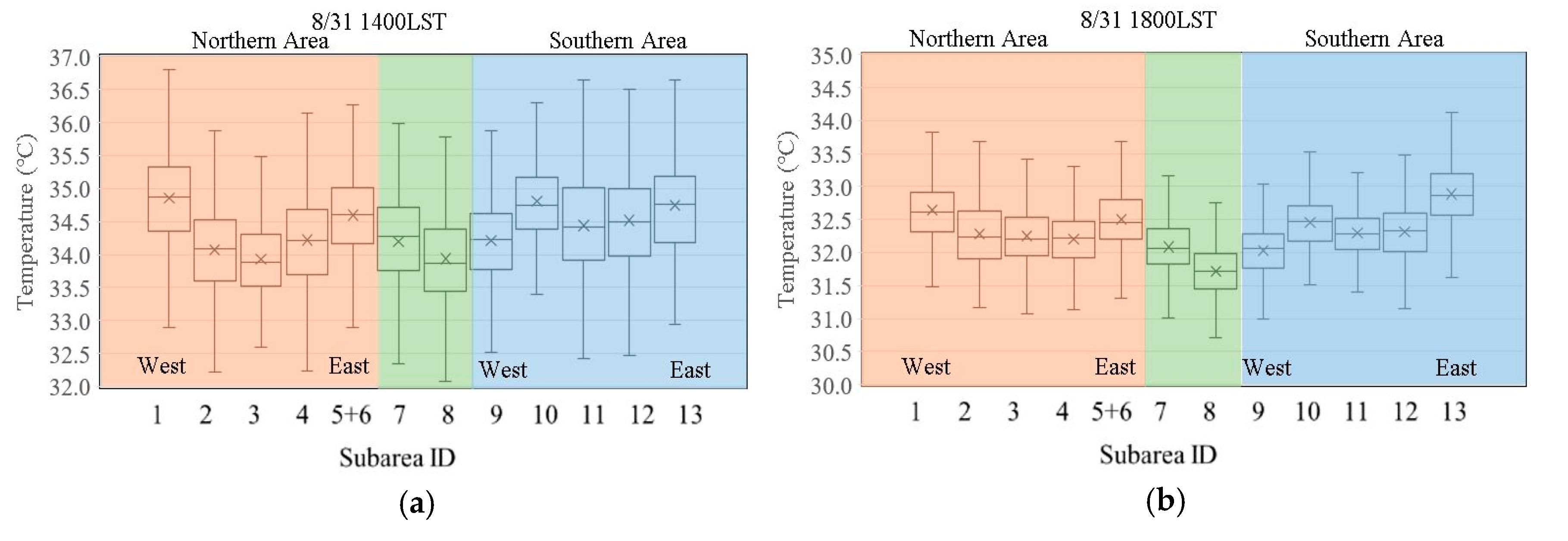
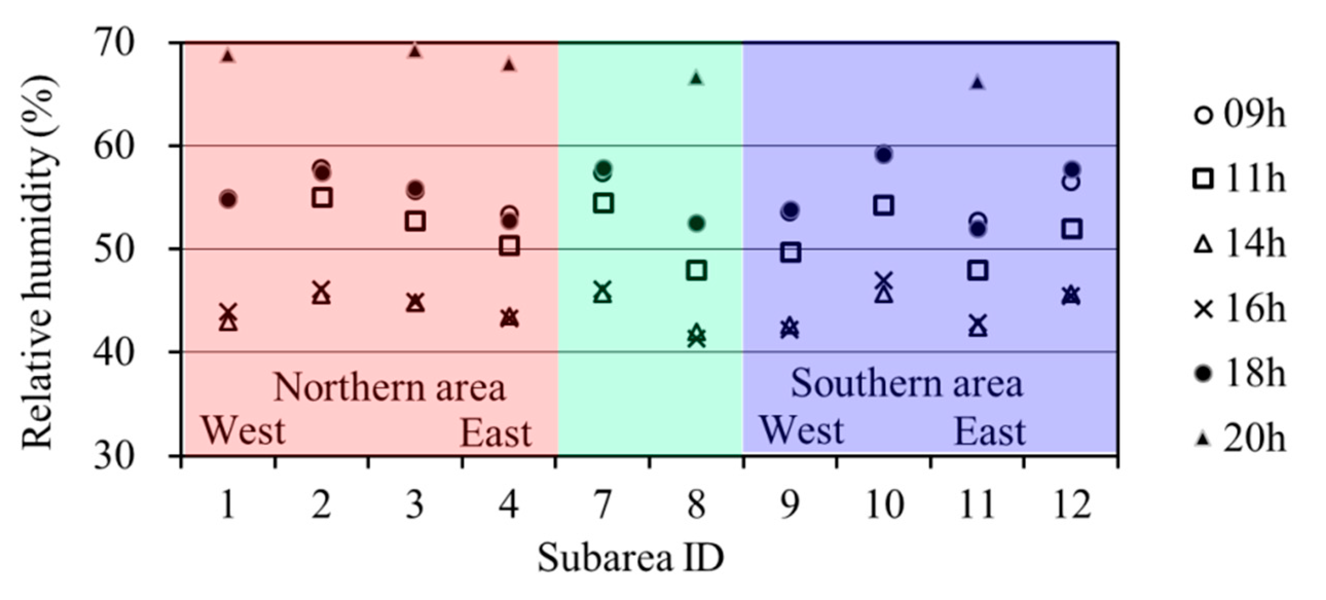
3.2. Temperature and Humidity Distributions in the Objective Area

As an example of mobile measurements, time series of the air temperature and the relative humidity variations on 31 August in the three subareas (1, 7, and 8) are shown in Figure 5, with the measurements obtained at the stationary point included in the subarea. Note that the record interval is 10 min at the stationary points and 1 s for the mobile observations. These data are raw measurements. No corrections have been applied. The time variations of the mobile observation data almost correspond to those obtained at stationary points. The temperature in subarea 1 is lower during the daytime (1100–1600 LST) and higher in the evening than the P1 data. This relationship also applies between subarea 7 and P2. The results obtained by traveling in the street canyons seem to exhibit urban canopy effect more intensely than the data of the stationary points located in relatively open places. On the other hand, in subarea 8, the mobile measurements of air temperature in the daytime are about 2 °C higher and the relative humidity is about 10% lower consistently than those observed at P4. The reason for this difference may be that P4 is in a humid place, in a green park near the river junction, while mobile measurements are obtained on paved streets.

After the data corrections for GPS route, instrumental error, time difference, and time responses, we made distribution maps of air temperature and relative humidity from the mobile measurements by interpolating them using the inverse distance weighted (IDW) method in ArcGIS.

In general, the air temperature variation in the study area is large in the daytime and small in the nighttime. However, the temperature distribution patterns are similar across days and hours. Here we show the characteristics of the distribution based on the results on 31 August as the examples. Figure 6 shows the air temperature distribution data obtained on 31 August. Air temperatures were generally lower within the Nakanoshima district (subareas 7 and 8) than in the outer areas. Outside the district, the temperatures in riverside areas along the Dojima and Tosabori Rivers were also relatively low. The mean temperature roughly increased from the west to the east, except in the most northwestern area (subarea 1). Relatively high temperatures were observed in the northern part of subarea 5 and 6 and in the southern part of subareas 11–13. These areas are crowded with office buildings and are distant from the rivers.

Figure 7 shows the statistical distribution of the air temperature at 1400 and 1800 LST on 31 August by box plots. The whiskers indicate the minimum and the maximum values excluding outliers, respectively. The lines of the box show lower quarter(Q1), median (Q2), upper quarter(Q3).

Q3–Q1 is called the IQR (interquartile range) which is 1.35 times the standard deviation (σ) in the case of the normal distribution. Data smaller than Q1-1.5 × IQR or larger than Q3 + 1.5 × IQR are regarded as outliers. In Figure 7, outlier plots are omitted to avoid visual complications. Mean values are shown in asterisks. The differences between Q2 and the mean value are small, less than 0.1 °C, for all runs of the observations. IQR/σ ranges 0.91–1.49 (1 July), 0.98–1.65 (29 July), and 1.16–1.50 (31 August). Clear relationship between IQR/σ and subarea or run is not found. At all times, Q2 in each subarea is near the midpoint of Q1 and Q3, which means that the skewness of the statistical distribution is not prominent.

The IQR in each subarea was relatively large (0.8–1.1 °C at 1400 and 0.5–0.7 °C at 1800), considering that the range of difference in median value of the temperature between the subareas was around 1 °C (1.0 °C at 1400 and 1.2 °C at 1800). These results suggest that the geometric characteristics of the urban block in a subarea (such as building density, building height, and road width) affect the mean temperature to some extent. We therefore investigated the relationship between the mean temperatures and geometric characteristics of the blocks. As a temperature index for an area, the deviation of the mean temperature of that area from the average value of all subareas was used. As geometrical indices of the urban blocks, the gross building coverage ratio and the mean number of stories of the buildings were used. Gross building coverage ratio (GBC), which represents building density, is defined as the ratio of the total area covered by buildings to the total ground area, and we estimated it from “Osaka City Mesh Data (2005)” provided by Planning and Coordination Bureau of Osaka City.

As shown in Figure 8a, mean temperatures tend to increase with GBC in both daytime and nighttime. Therefore, it seems that the low temperatures in the Nakanoshima district are due to the area’s low building density; the ventilation efficiency of an area promotes sea breeze cooling in the daytime, which reduces heat storage in the ground and the bodies of buildings and leads to low temperatures in the nighttime. Additionally, as shown in Figure 8b, the mean temperature in a subarea tends to decrease as the mean number of stories of buildings (S) increases. One of the reasons for this correlation is the effect of shadows during the daytime. Another possible reason is the increase in wind speed at ground level around tall buildings, which is induced by turbulent eddies. Both of these effects will reduce heat storage in the daytime. Figure 8c shows the correlations between the s.t.d. of air temperature (σ_T) and GBC. From the daytime to the evening, σ_T are reduced in all subareas. The decrease in σ_T in the outer subarea of the Nakanoshima district is smaller than in the inner subarea. In the outer subareas, effect of diurnal variation in radiation on air temperature may be relatively small because urban canopy effect is prominent by their high building density. In a low GBC area, such as the inner subareas of Nakanoshima district, open spaces occupy a large portion of it. In there, radiative cooling develops in the evening, and it uniformly lowers the air temperature on the open surface. Therefore, the σ_T decreases significantly from daytime to the nighttime. As a result, the correlation between GBCs and σ_T is inverted between the daytime and the nighttime. The relationship between the σ_T and S were shown in Figure 8d. As in the case of the mean temperature difference, the correlation with S shows the opposite tendency to the case in GBC. Note that the correlations between the geometrical indices and the deviation of mean temperature are significant. On the other hand, the relationships between the geometrical indices and σ_T are not significant.

Figure 9 shows the distribution of relative humidity on 31 August. Because thermo-only sensors were used in subarea 6 and 13, relative humidity in the most eastern part of the study area was not obtained. The distribution pattern of specific humidity is similar to that of relative humidity, possibly due to the temperature difference in the objective area being relatively small. In general, the pattern of humidity distribution correlated inversely with that of temperature; high humidity was found in the riverside zones of the Dojima and the Tosabori Rivers. Figure 10 shows the mean relative humidity in each subarea. The main features of the relative humidity distribution, as opposed to the temperature distribution, can be summarized as follows: both temperature and humidity were higher on the western side of the Nakanoshima district (subarea 7), which is near a confluence of the rivers, than on the eastern side of the district (subarea 8); a high humidity zone can be seen at the southern edge of the observation area, where there is a large green park.

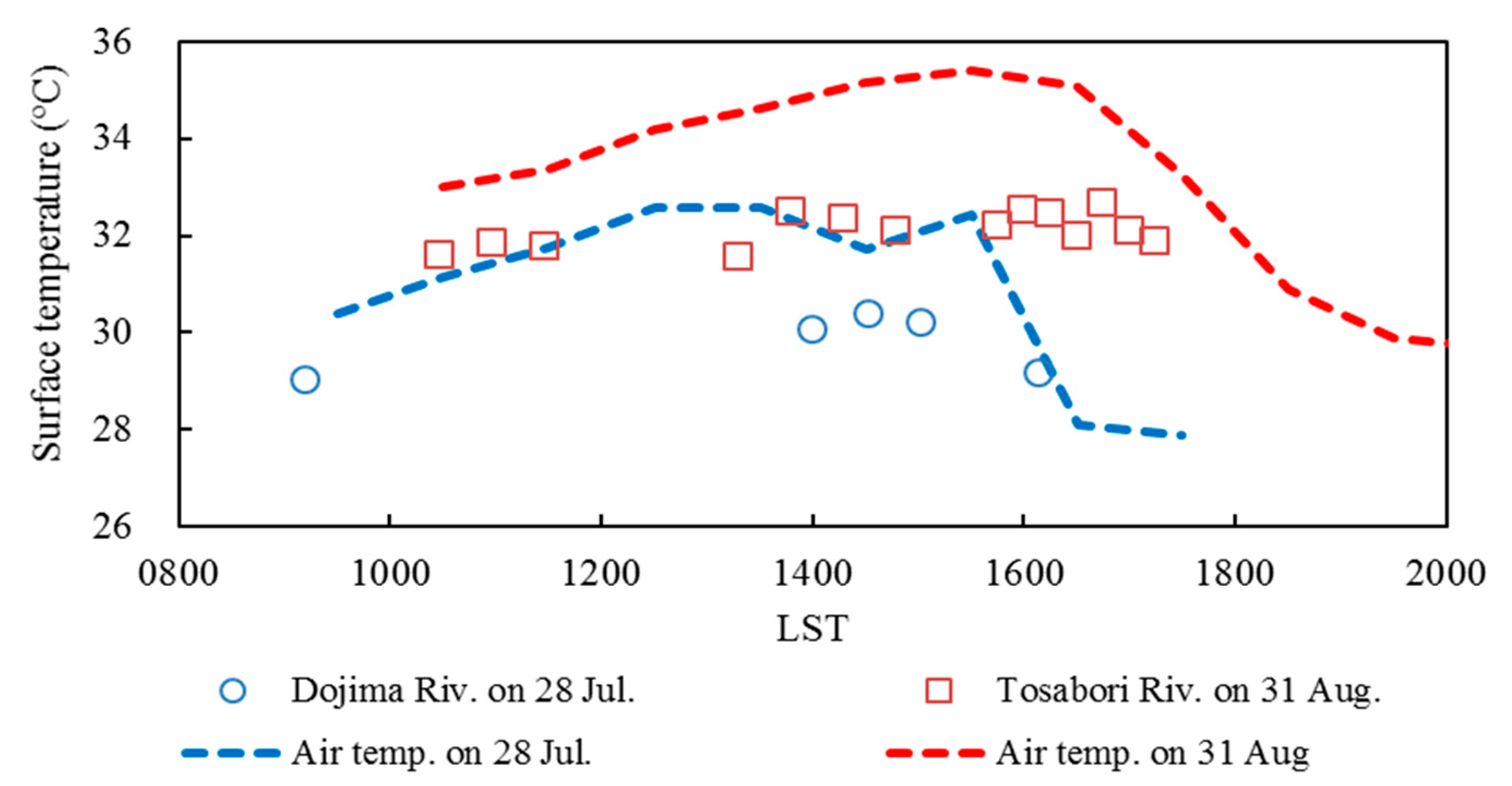
3.3. Characteristic of Upper Wind and River Surface Temperature

Figure 11a shows an example of the upper wind profiles obtained on 31 August. Some discontinuous changes in wind direction and wind speed (e.g., wind speed at 1112 LST, both wind direction and wind speed at 1820 LST) were observed at around 1 km AGL. In the lower layer, the wind direction was between S and W, and the wind speed was light to moderate (3–6 m/s), which suggests that the depth of the sea breeze layer during this observation period was approximately 1 km. As shown by the trajectories of pilot balloons (Figure 11b), the direction of the sea breeze, unlike the surface wind direction, does not necessarily coincide with the paths of the rivers sandwiching the Nakanoshima district (see Section 3.1). On the other hand, wind direction above the sea breeze layer was variable; it is likely to depend on the synoptic conditions. Wind speed above the sea breeze layer was often lower than that in the layer because our observation was executed under typical anticyclone conditions. These features of the wind profiles were often observed on other days and hours during the observation period.

Figure 12 shows the diurnal variations in the surface temperatures of the rivers sandwiching Nakanoshima, as obtained using thermography on 31 August. The surface temperatures of the rivers increase with air temperature, though the increment of the surface temperature is smaller than that in air temperature, and the rivers therefore act as heat sinks in the daytime. The surface temperatures of the rivers were generally lower than the air temperature at P2 from 0900 to 1700 LST, and the maximum difference is about 2 °C.

4. Conclusions

In the observation area, large temperature differences were found even within a relatively small area. The building density seems to affect the mean air temperature because it influences the ventilation efficiency of the area. The temperature of the Nakanoshima district is generally lower than that of its surrounding area because the building density is relatively low. The relative humidity distribution was inversely correlated with the air temperature distribution in general; however, both temperature and relative humidity were high at the confluence of the rivers and green parks. The depth of the sea breeze layer penetrating the Nakanoshima district was found to be about 1 km. The sea breeze direction near the ground is aligned with but opposite to the direction of the rivers surrounding the Nakanoshima district. During the daytime, 0900 to 1700 LST, the surface temperature of the rivers sandwiching the district was lower than the air temperature observed at the nearest stationary observation point, and the difference reached approximately 2 °C.

References

1. Oke, T.R. Boundary Layer Climates, 2nd ed.; Routledge: London, UK, 1987. [Google Scholar]
2. Komatsu, H. Evaluation of recent hot summer in Kansai: Basic information for supply and demand of electricity. Jpn. J. Biometeorol. 2014, 51, 37–47. [Google Scholar]
3. Ono, M. Chapter 3-Heat stroke in the summer of 2010. In Meteorological Research Note; The Meteorological Society of Japan: Tokyo, Japan, 2012; Volume 225, pp. 29–35. [Google Scholar]
4. Yokoyama, T.; Fukuoka, T. Regional tendency of heat disorders in Japan. Jpn. J. Biometeorol. 2006, 43, 145–151. [Google Scholar]
5. Hoshi, A.; Nakai, S.; Kaneda, E.; Yamamoto, T.; Inaba, Y. Regional characteristics in the death due to heat disorders in Japan. Jpn. J. Biometeorol. 2010, 47, 175–184. [Google Scholar]
6. Fujibe, F. Long-term variations in heat mortality and summer temperature in Japan. Tenki 2013, 60, 371–381. [Google Scholar]
7. Fujibe, F. Evaluation of background and urban warming trends based on centennial temperature data in Japan. Pap. Meteorol. Geophys. 2012, 63, 43–56. [Google Scholar] [CrossRef]
8. Ono, M.; Ueda, K. Chapter 16—Prediction of heat stroke damage by global warming. In Meteorological Research Note; The Meteorological Society of Japan: Tokyo, Japan, 2012; Volume 225, pp. 177–182. [Google Scholar]
9. Adachi, A.S.; Kimura, F.; Kusaka, H.; Inoue, T.; Ueda, H. Comparison of the impact of global climate changes and urbanization on summertime future climate in the Tokyo metropolitan area. J. Appl. Meteorol. 2012, 51, 1441–1454. [Google Scholar] [CrossRef]
10. Ministry of the Environment, Government of Japan. Heat Stress Index: WBGT, Heat Illness Prevention Information (Online). Available online: http://www.wbgt.env.go.jp/en/ (accessed on 1 July 2020).
11. Kono, H.; Narumi, D.; Shimoda, Y. Osaka, Klimaatlas for Urban Environment; Gyosei Co.: Tokyo, Japan, 2000; pp. 53–65. [Google Scholar]
12. Fire and Disaster Management Agency. Heatstroke Information. Available online: https://www.fdma.go.jp/disaster/heatstroke/post1.html (accessed on 1 October 2020).
13. Osaka City, “Kaze-no-Michi” Vision [Basic Policy]. 2011. Available online: http://www.city.osaka.lg.jp/kankyo/page/0000123906.html (accessed on 1 July 2020).
14. Kubota, T.; Miura, M.; Tominaga, Y.; Mochida, A. Wind tunnel tests on the nature of regional wind flow in the 270 m square residential area, using the real model, Effects of arrangement and structural patterns of buildings on the nature of regional wind flow Part 1. J. Archit. Plan. Environ. Eng. 2000, 529, 109–116. [Google Scholar]
15. Takebayashi, H.; Moriyama, M.; Miyake, K. Analysis on the relationship between properties of urban block and wind path in the street canyon for the use of the wind as the climate resources. J. Environ. Eng. 2009, 74, 77–82. [Google Scholar] [CrossRef] [Green Version]
16. Wong, M.S.; Nichol, J.E.; To, P.H.; Wang, J. A simple method for designation of urban ventilation corridors and its application to urban heat island analysis. Build. Environ. 2010, 45, 1880–1889. [Google Scholar] [CrossRef]
17. Nabeshima, M.; Kozaki, Y.; Nakao, M.; Nishioka, M. Experimental study of heat island phenomena by mobile measurement system, Horizontal air temperature distribution at night in the Osaka plain. J. Heat Island Inst. Int. 2006, 1, 23–29. [Google Scholar]
18. Mizuno, M.; Nabeshima, M.; Nakao, M.; Nishioka, M. Study on temperature distribution of an urbanized area using a vehicle with mobile measurement system: Analysis on characteristics of the 330 horizontal distribution using semivariogram and kriging. J. Environ. Eng. 2009, 74, 1179–1185. [Google Scholar] [CrossRef]
19. Sahashi, K. Errors in the air temperature observation by traveling method with the automobiles: Effects of the automobiles. Tenki 1983, 30, 509–514. [Google Scholar]
20. Melhuish, E.; Pedder, M. Observing an urban heat island by bicycle. Weather 1998, 53, 121–128. [Google Scholar] [CrossRef]
21. Takayama, N.; Yamamoto, H.; Zhang, J.; Iwaya, K.; Wang, F.; Harada, Y.; Kaneishi, A.; Tsuchiya, Y.; Mori, H. Development and application of mobile observation method of urban climate to analyze occurrence of heat-island in Changchung city of China. Archit. Inst. Jpn. Technol. Des. 2009, 15, 827–832. [Google Scholar] [CrossRef] [Green Version]
22. Brandsma, T.; Wolters, D. Measurement and statistical modeling of the urban heat island of the city of Utrecht (the Netherlands). J. Appl. Meteorol. Climatol. 2012, 51, 1046–1060. [Google Scholar] [CrossRef] [Green Version]
23. Nakao, M.; Nabeshima, M.; Hasegawa, M.; Nishioka, M. Continuous mobile measurement method to estimate thermal environmental distribution in street. In Architectural Institute of Japan, Summaries of Technical Papers of Annual Meeting (Chugoku); Architectural Institute of Japan: Tokyo, Japan, 2008; pp. 981–982. [Google Scholar]
Figure 1. Maps of the study area; (a) Geographical feature of Osaka area. A white line and a dark-red line are the borders of Osaka Prefecture and Osaka City, respectively. (b) Study area (enclosed by the white line) and stationary observation points. Stationary observation of air temperature, relative humidity, and wind at ground level were executed at P2. The same elements were observed at P0 by the Osaka Meteorological Observatory and at P1 and P4 by The General Environmental Technos Co., LTD. Upper winds were observed at P2 using pilot balloons. Surface temperature on the rivers were observed from a building at P3. Yellow arrows indicate mean wind directions in the daytime at P1 and P4, respectively. (c) Subareas for mobile observations (13 divisions. 28 July. and 31 August., 2010). Serial number in the figure indicates the ID of each subarea. Area of the Nakanoshima district corresponds to subarea 7 and 8.
Atmosphere 11 01234 g001
Figure 2. Equipment for the mobile observation. (a) A double tube with a cooling fan; (b) Arrangement of the instruments on a bicycle.
Atmosphere 11 01234 g002
Figure 3. Travelling routes of the mobile observation started at 1400 LST, 31 August 2010. Different colors were used to distinguish adjacent subareas. The same color was used for different subareas if it was not confusing (see Figure 1c).
Atmosphere 11 01234 g003
Figure 4. Time variations of meteorological elements on 31 August 2010. (a) SR: global solar radiation, T: Air temperature, (b) RH: Relative humidity. (c) WS: Wind speed, WD: Wind direction. P1, P2, and P4 are the stationary points. P0 is the Osaka Meteorological Observatory nearby the study area (see Figure 1b).
Atmosphere 11 01234 g004
Figure 5. Time series variations of the air temperature and the relative humidity obtained at a stationary point and mobile observations in the subarea on 31 August. (a) P1 and Subarea-1, (b) P2 and Subarea-7, (c) P4 and Subarea-8.
Atmosphere 11 01234 g005
Figure 6. Horizontal distribution of air temperature on 31 Aug. 2010. (a) 1400 LST, (b) 1800 LST.
Atmosphere 11 01234 g006
Figure 7. Box plots of the air temperatures in each subarea on 31 August 2010. (a) 1400 LST, (b) 1800 LST. Subarea IDs are shown in Figure 1c. Green background shows subareas in the Nakanoshima district. Subarea 5 and 6 were merged on this day.
Atmosphere 11 01234 g007
Figure 8. Relationships between (a) gross building coverage ratio (GBC) and deviation of mean temperature (DT), (b) the mean number of stories (S) and DT, (c) GBC and standard deviation of temperature in a subarea (σT), and (d) S and σT. The symbols in a box of thick line are the data within the Nakanoshima district (subarea 7 and 8). **: p < 0.01, *: p < 0.05.
Atmosphere 11 01234 g008
Figure 9. Horizontal distribution of relative humidity on 31 August 2010. (a) 1400 LST, (b) 1800 LST.
Atmosphere 11 01234 g009
Figure 10. Mean relative humidity in each subarea on 31 Aug. 2010. Subarea IDs are shown in Figure 1c. Data of subarea 5, 6, and 13 does not exist because observations in these subareas were made with thermo-only sensors. Green background shows subareas in the Nakanoshima district.
Atmosphere 11 01234 g010
Figure 11. Upper wind around the study area on 31 August 2010. (a) Vertical profiles of the horizontal winds. The numbers in the figures are starting time (hhmm LST) of the observations. (b) Three-dimensional trajectories of the pilot balloons. The circular mark indicates balloon position of every 20 s (vertical interval is approx. 50 m). The starting time of each observation is shown near the end point of the trajectory.
Atmosphere 11 01234 g011
Figure 12. Surface temperature of the rivers and air temperature at ground level. The surface tempera-tures of the rivers were observed from a balcony of a hi-rise building at P3, using an IR thermography camera (see Figure 1b). The air temperature was observed at P2.
Atmosphere 11 01234 g012