Article

A Machine Learning Approach to Investigate the Surface Ozone Behavior

by
Roberta Valentina Gagliardi
1,* and
Claudio Andenna
2
1
Istituto Superiore di Sanità, Viale Regina Elena 299, 00161 Rome, Italy
2
INAIL-DIT, Via del Torraccio di Torrenova 7, 00133 Rome, Italy
*
Author to whom correspondence should be addressed.
Atmosphere 2020, 11(11), 1173; https://doi.org/10.3390/atmos11111173
Submission received: 25 September 2020 / Revised: 24 October 2020 / Accepted: 28 October 2020 / Published: 30 October 2020

Abstract

:
The concentration of surface ozone (O3) strongly depends on environmental and meteorological variables through a series of complex and non-linear functions. This study aims to explore the performances of an advanced machine learning (ML) method, the boosted regression trees (BRT) technique, in exploring the relationships between surface O3 and its driving factors, and in predicting the levels of O3 concentrations. To this end, a BRT model was trained on hourly data of air pollutants and meteorological parameters, acquired, over the 2016–2018 period, in a rural area affected by an anthropic source of air pollutants. The abilities of the BRT model in ranking, visualizing, and predicting the relationship between ground-level O3 concentrations and its driving factors were analyzed and illustrated. A comparison with a multiple linear regression (MLR) model was performed based on several statistical indicators. The results obtained indicated that the BRT model was able to account for 81% of changes in O3 concentrations; it slightly outperforms the MLR model in terms of the predictions accuracy and allows a better identification of the main factors influencing O3 variability on a local scale. This knowledge is expected to be useful in defining effective measures to prevent and/or mitigate the health damages associated with O3 exposure.

1. Introduction

The generalized interest in analyzing the behavior of ground level ozone (O3), which is a secondary pollutant in the atmosphere, is due to its proved adverse human health effects [1,2,3,4] and its detrimental impact on vegetation [5,6,7,8] and materials [9,10,11]. The exposure to surface O3 increases morbidity levels and premature mortality in a population. According to the World Health Organization (WHO) [12], there is strong evidence, from epidemiological and toxicological studies, that surface O3 is causally associated with adverse respiratory effects. These effects range from changes in lung function and asthma to mortality, especially amongst sensitive risk groups in the population (children, elderly people, and individuals with respiratory illnesses). As established by the European Environmental Agency [13], in 2017, as much as approximately 96% of the total EU-28 urban population was exposed to O3 levels exceeding the threshold for the protection of human health (8 h mean of 100 μg/m3) set by the WHO Air Quality Guidelines [14]. No less important is the influence of tropospheric O3 on climate change, to which it contributes by acting both as a greenhouse gas and as an indirect controller of others greenhouse gases lifetimes [15,16,17]. Moreover, growing interest has recently emerged on the role played by O3 and by other pollutants (particulate matter and nitrogen oxides) as potentially related to coronavirus (Covid-19) diseases [18].
The level of surface O3 in a given area is controlled by various chemical and dynamical processes acting as sources (chemical production, stratospheric intrusions, long-range transport) and sinks (chemical destruction, dry deposition). The primary source of surface O3 formation is represented by a chain of photochemical reactions with the involvement of precursor gases including nitrogen oxides (NOx = NO + NO2), carbon monoxide (CO), methane (CH4) and non-methane volatile organic compounds (NMHC) [15]. Henceforth, CO, CH4, NMHC, NOx, NO2, NO will be referred collectively as the O3 precursors. The efficiency of the photochemical reactions depends on the concentrations of precursors and on the meteorological parameters. Furthermore, the latter affect the natural emission of precursors and the processes of accumulation, dispersion, transport, and removal connected to the air pollutants [19]. Therefore, the surface O3 variability is highly dependent on precursors, meteorological parameters, and their interactions through a series of complex and non-linear functions.
Statistical modeling techniques have been extensively used in the air pollution field to characterize the relationships between variables. The statistical techniques based on regression models, such as the multiple linear regression (MLR), are frequently applied to establish a relationship between several explanatory variables (predictors) and a response variable (target). However, in spite of their evident capability of providing reasonable results in many applications, these kinds of models tend to fail in describing the complexity of non-linear relationships and interactions between variables, and more sophisticated techniques are generally preferred to obtain a better accuracy in predictions of pollutants concentration levels [20].
In the last three decades, advanced statistical models based on machine learning (ML) techniques have been developed and increasingly applied in the air quality modeling field [21] due to their capabilities of exploring large and complex datasets (big data), discovering patterns, and making predictions. The core objective of a ML algorithm is to provide a model that captures the overall characteristics and interactions of the dataset on which it has been trained in order to gain knowledge from data and make predictions [22]. Some of the most promising ML algorithms for detecting non-linear relationships among variables include methods based on the decision trees, such as the boosted regression trees (BRT) and random forest (RF) techniques. Both algorithms have shown good performances over a wide range of environmental issues [23]. The RF method has been widely applied to estimate particulate matter, NO2, and O3 exposure at different spatial scale [24,25,26,27]. Few works investigated the relevance of input variables in O3 concentration prediction using the BRT algorithm [28], although several studies, comparing different machine learning models, pointed out the BRT strong predictive performance and remarkable capability of insights on the relationships between variables [29,30,31]. The BRT is a classification and regression method that combines the strengths of two algorithms: the regression tree model that relates a target variable to explanatory variables by recursive binary splits, and a boosting technique, which combines many simple weak tree-based models to improve performances [32]. Its strength lies in the capacity to model the relationship between the target variable and predictors in a flexible way, also taking into account the non-linear effects and the interactions among variables, which are often the norm for many air pollution processes. Among competing ML techniques that are highly relevant to the air quality studies, the use of the BRT is generally preferred where the model interpretation is a priority [29,33]; in fact, it provides several outputs, which are useful in interpreting the model in a physically and chemically meaningful way.
The aim of this study was to characterize the surface O3 behavior using the potentialities of the BRT technique both as a diagnostic tool, to explore the relationships between surface O3 and several influential factors, and as a predictive tool, to forecast O3 concentration levels. To this end, a BRT model was developed and tested on a data set comprising hourly data of air pollutants (O3 and its precursors) and meteorological parameters. Data were collected, over the 2016–2018 period, at a monitoring site affected by an anthropic source of air pollutants potentially influencing the O3 levels, located in the center of the Mediterranean area, one of the most responsive regions to climate change. The BRT model outputs were analyzed to elucidate the role of different drivers of the surface O3 variability. In addition, a MLR model was developed to compare the performances and the predictive ability of both models through a set of appropriately selected statistical indicators. A deeper knowledge on the factors affecting the O3 formation and its variations on a local scale is expected to be useful for the effective management of public protection activities from O3 exposure. Similarly, this knowledge could support the development of win-win strategies that maximize co-benefits of O3 reduction for both air quality and climate changes [16,34]. Moreover, the urgent question concerning the role of air pollution and meteorological factors on the COVID-19 outbreak spreading [35] could profit by a deeper insight of the relationships among variables obtainable through a machine learning approach.

2. Materials and Methods

2.1. Study Area

The study area is the Agri Valley, located in the south-west part of the Basilicata Region (Southern Italy) (Figure 1); the valley, which is located at approximately 600 m a.s.l., is bordered on both sides by the Apennine Mountains and hosts a population of approximately 50,000 inhabitants distributed in several small hilltop towns surrounding the valley. The area represents a predominantly rural environment, comprising woods, agricultural and breeding zones, partially included in a National Park (Appennino Lucano, Val d’Agri, Lagonegrese National Park). In general, the climate of the area is sub-continental, characterized by cold and rainy winter as well as cool summers with frequent rainfall [36]. Furthermore, the site is characterized by the presence of the largest on-shore western European reservoir of crude oil and gas and of an oil pre-treatment plant (identified as Centro Olio Val d’Agri—hereafter COVA) in a populated area. The industrial processes taking place at the COVA plant, operating since 2001, produce conveyed and diffuse emissions of gases and particulate, which can affect the air quality and potentially pose health risks for the population living in the area. Moreover, the site is located in the center of the Mediterranean area, which is considered a “hot spot” for climate change due to the intense photochemical activity, the crossing of air masses of different origin, and the strong anthropogenic pressure. These conditions make the area interesting for future insights on the interconnections between air quality and climate changes [37].
An air quality control network, consisting of five monitoring stations, is arranged in the Agri Valley, providing continuous concentration measurements of regulated pollutants (CO, CH4, NOx, NO2, NO, O3) and of several pollutants specifically related to oil/gas extraction activities (NMHC). The following meteorological parameters are measured at the stations: temperature (T), atmospheric pressure (P), relative humidity (RH), solar radiation (SR), wind direction (wd), and wind speed (ws). The Environmental Protection Agency of the Basilicata Region (ARPAB), managing the network, validates and makes public the data. More details about the methods and the instrumentation used for the measurements can be found elsewhere [38,39]. For the purpose of this work, data were obtained from the station named Masseria De Blasis (MdB, 40°19′27″ N, 15°52′02″ E), an industrial station in a rural area, already subjected to a preliminary investigation [40]. It is located at the same altitude of the COVA plant, namely 603 m a.s.l., at approximately 2800 m from the industrial site and approximately 250 m from a high-speed motorway (SS598).

2.2. Data Preparedness

Based on the open data measured and validated by ARPAB, several available parameters were selected to prepare the database on which developing the BRT and MLR models.
Therefore, variables representing O3 precursors were included among predictors together with the following meteorological variables: T, RH, SR, P, ws, and wd. Overall, a data set consisting of 13 variables and more than 25,000 observations covering the 2016–2018 period was set up. This timeframe was defined selecting the most complete time series and the most updated available data. The time series of all predictors considered respected the required 75% proportion of valid data. The final dataset was divided into two parts: the first one, concerning the data of the period from 2016 to 2017, was used to build the BRT and the MLR models; while the second one, the validation dataset based on the data from 2018, was used to investigate the predictive ability of both models. In the case of the BRT model development, the first dataset was again randomly divided into a training set (80%), used to train the model, and a testing set (20%) to test the performances of the model.

2.3. BRT Model Devolopment

The BRT technique, whose theoretical foundations are described in detail in [31,32], does not require pre-processing of data. It works successfully with both continuous and categorical variables, it handles missing data and it is not sensitive to outliers. However, to fit the algorithm to the dataset under examination, the BRT technique requires setting several parameters to control the learning process. The process of choosing the optimal values for these parameters is referred to as the tuning process of hyperparameters. Generally, the main hyperparameters to be taken into account are: the learning rate (lr, controlling the rate of model complexity increasing), the tree complexity (tc, the number of nodes in a tree), and the bag-fraction (bf, specifying the proportion of data randomly selected to fit each consequent tree). Finally, nt indicates the number of trees required for an optimal prediction.
Therefore, to fit the algorithm to the dataset under examination, a two-step process was carried out: first, potential models were built using the training dataset for each combination of hyperparameters specified on a grid; second, the combination of the best performing hyperparameters on the testing dataset was selected. The model trained with this resulting combination of hyperparameters was chosen as the final model. In the present study, the optimal values of hyperparameters thus determined were, respectively, lr = 0.01, tc = 6, bf = 0.5, and nt = 8150.

2.4. MLR Model Development

A MLR model based on the backward elimination for variables selection was developed using the dataset covering the 2016–2017 period. Before implementing the MLR procedure, the explanatory variables were standardized by subtracting the mean and dividing by the standard deviation to avoid the scale effect.
The MLR technique requires several assumptions to be satisfied: (1) no multi-collinearity in the data, i.e., explanatory variables independent from each other, and (2) normal distribution of the residual errors with zero mean and constant variance [41,42]. To check the multi-collinearity between variables, the variance inflation factor (VIF) was used as a diagnostic tool. The criterion of VIF greater than 10, representing serious levels of multi-collinearity, was adopted to exclude the critical variables from the regression [43]. In addition, a graphical analysis of the residuals was performed to detect violations of the normality of residuals and homogeneity of variance. Finally, F-test and t-test were conducted to verify the statistical significance of both the overall relationship represented by the regression model developed and the individual parameters. Among all variables, only those respecting the statistical significance levels (p-value < 0.05) were retained.

2.5. Models Evaluation

Once developed, the performances of the BRT and MLR models in predicting the O3 concentration was verified using the validation data set. The accuracy and the errors of both models were evaluated through several statistical indicators, namely the coefficient of determination (R2), the index of agreement (IoA), the mean bias error (MBE), the mean absolute error (MAE), and the root mean square error (RMSE), whose equations are provided in Appendix A [44,45]. High accuracy (R2 and IoA close to 1) and minimal errors (MBE, MAE, and RMSE close to 0) are the desired performances for an optimal prediction model. Some graphical functions, as, for example, the scatter plots, were also utilized to support the analysis of the strengths and the criticalities of both the developed models.
All the analysis was accomplished in the R 3.6.1 software environment [46], mainly using the Openair package for air quality data analysis [47], the stats package, and the gbm package for the development of the MLR and the BRT model [48], respectively.

3. Results and Discussion

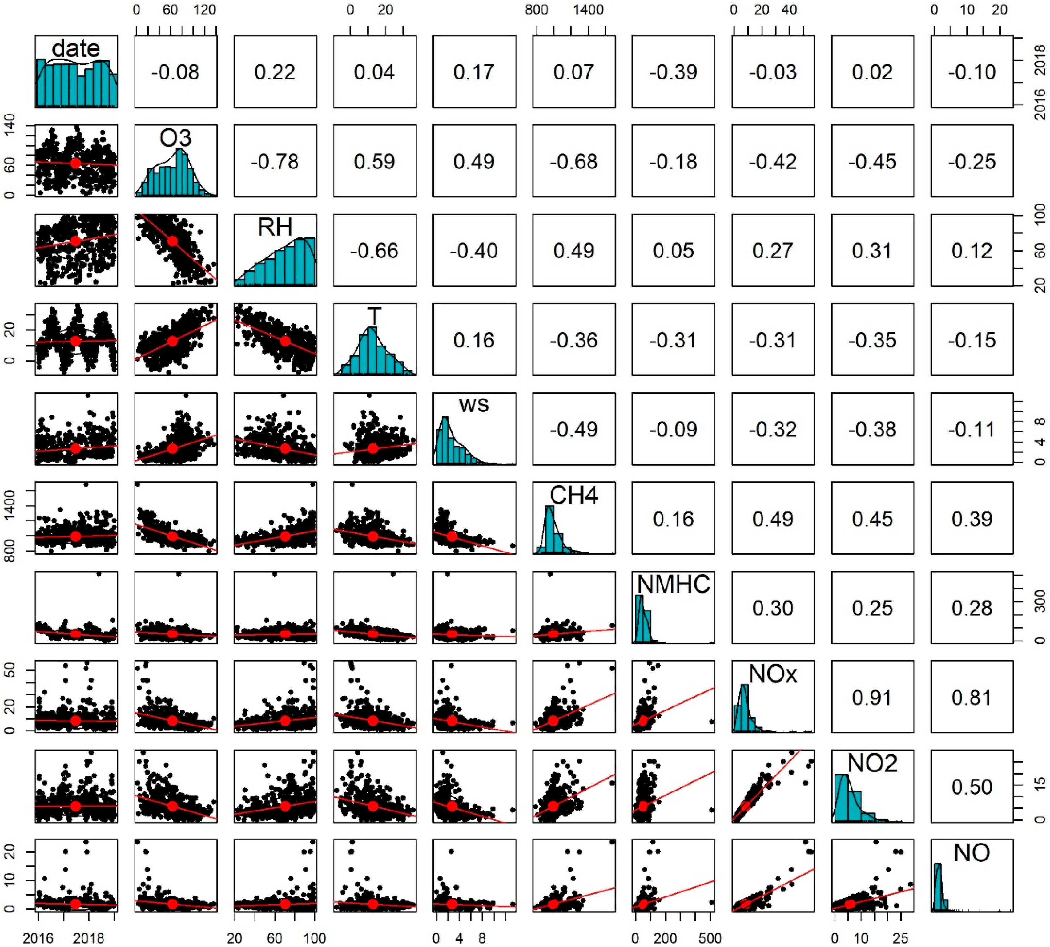
3.1. Statistical Analysis
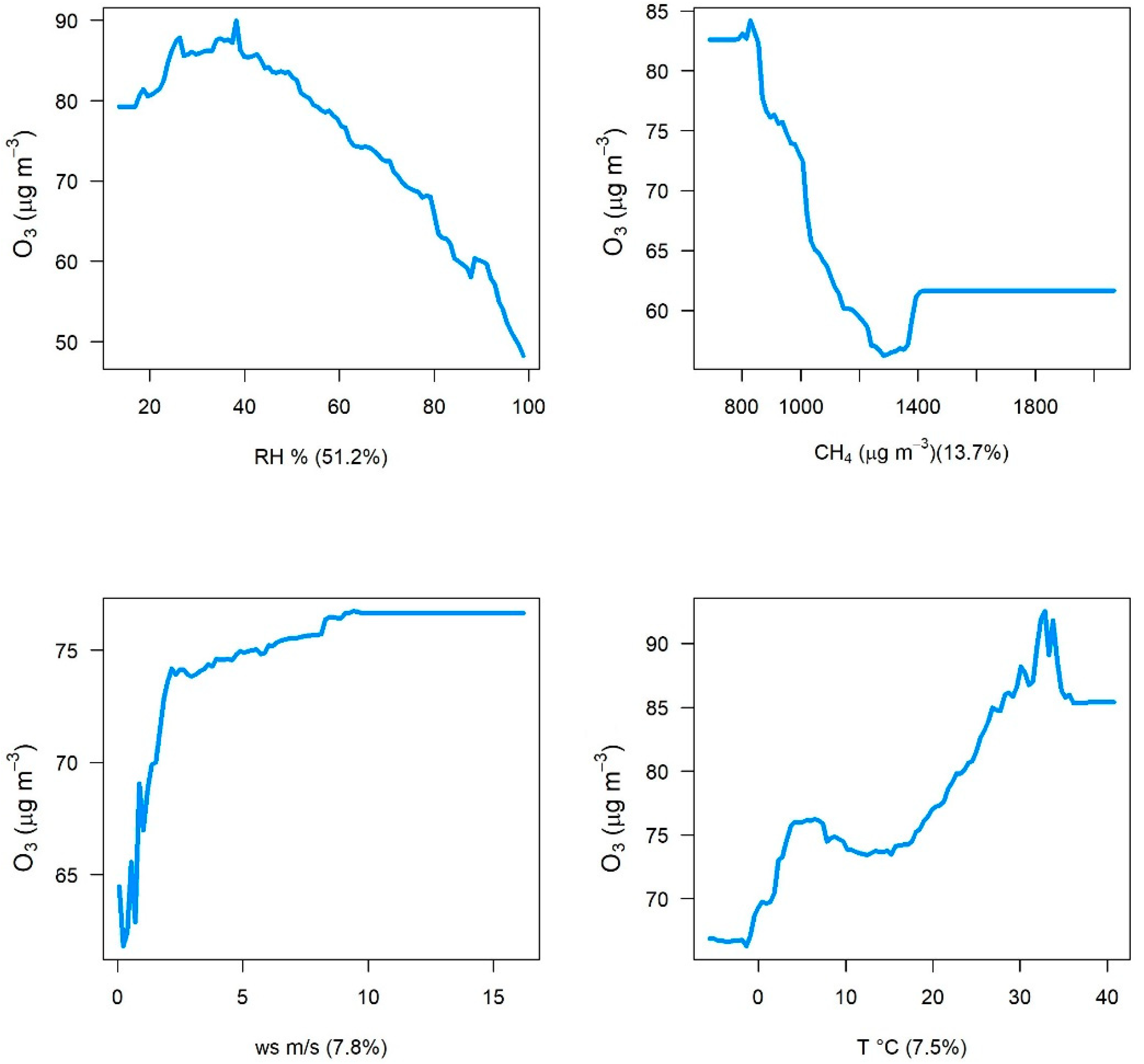
The data statistical analysis for the whole period considered is presented in Table 1. The O3 limit values for the protection of human health are set in the European Legislation [49]. O3 hourly average concentrations were between 0.20 and 229.20 µg/m3, with a mean value of 63.23 µg/m3. Two exceedances of the information threshold, set to 180 µg/m3, were registered in July 2016, while conformity to the alert threshold, set to 240 µg/m3, was observed for the entire examined period.
The target value for the protection of human health, i.e., 120 µg/m3, as maximum daily eight-hour mean, not to be exceeded on more than 25 days per year, as a mean of three years, was not reached. However, the threshold for the human health protection set by the WHO [14], (8 h mean of 100 μg/m3), was surpassed in all three years during the summer season. For the other regulated pollutants included in the present analysis, the concentrations levels resulted lower than the threshold values set by the national legislation currently in force [50]. It is also worth noting that the NMHC concentration levels, not regulated by law either at the European or at national level, exhibited a peculiar trend, which is characterized by several concentration spikes well above its average or background level. During the study period, the mean temperature was 13.0 °C; the minimum value was recorded in January 2017 in correspondence with of an exceptional cold wave involving the entire national territory. Relative humidity ranged from 58.2% of July to 81.3% of November with a mean value of 71.21%, while pressure was rather static. The mean value of ws was 2.76 m s−1, with the higher values generally measured during daytime. As results from the wind rose in Figure 1, the prevailing wind direction was from the west sector and, in the second instance, from the north-west sector, determining an upwind position of the MdB station with respect to the COVA plant.
A Pearson correlation analysis was performed to identify the strength of the relationships between pairs of variables. The most significant results are summarized in Figure 2.
Among the meteorological parameters, the highest negative correlation was found between O3 and the RH (R = −0.78), while a positive correlation was registered with T (R = 0.59) and ws (R = 0.49), respectively. O3 was negatively correlated with all the precursor gases, in particular CH4 was the most efficient one (R = −0.68). Finally, a strong positive correlation was found between NOx and NO2 (R = 0.91), and a negative correlation between RH and T (R = −0.66). All the obtained results are generally congruent with the expected trends and they will be discussed in details in the paragraph dedicated to the BRT model results.

3.2. BRT Results

The outcomes of the BRT algorithm were obtained training the following model over the period 2016–2017:
O 3 ~ gbm ( T , H , ws , wd , P , SR , NO , NO 2 , NO x , CH 4 , NMHC , CO ) ,
where gbm is the function implementing the boosted regression tree technique in the R software environment. Several tools allow interpreting the BRT model, enhancing its understanding and trustworthiness, i.e., the relative influence of predictors, the partial dependence plots, and the two-way predictor interactions.
The relative influence, ranking in a descending order the most influential predictors, indicates to what extent each predictor influences the target variable. According to the obtained results (Figure 3), the overall contribution of meteorological variables explained over 70% of the variance in O3, indicating that meteorology, at a local scale, was a strong driver for O3 concentrations in the area. The most important meteorological parameters were RH, ws, and T, the others making a negligible contribution. Remarkable was the role of RH, explaining alone more than 50% of the variance in the BRT model. Among the precursor gases, the most relevant was CH4, showing an influence of 13% on O3, while nitrogen gases accounted for percentage values of less than 6%.
The partial dependence plots describe how the target variable is changing in terms of the chosen predictor, after accounting for the average effects of all other explanatory variables; it provides a useful basis to visualize the relationships between O3 and its driving factors. With reference to the top four predictors identified by the BRT model (Figure 4), some considerations can be formulated.
The strong negative association found between O3 concentrations and RH can be due to several factors. Relative humidity influences photochemistry through reactions between water vapor and atomic oxygen, increasing O3 chemical losses [51]. In addition, photochemistry reduction, due to the enhanced cloud cover associated with high humidity levels, is another plausible explanation. Furthermore, RH influences O3 concentration also by dry deposition, for example, enhancing plants stomatal opening and consequently O3 uptake [52]. Although not easily quantifiable, this is expected to be a non negligible phenomenon in the area under examination due to the relevant presence of vegetation near the monitoring site.
O3 was negatively correlated with CH4 as expected, since this pollutant is known to be a precursor of O3 [53]; CH4 oxidation, in fact, leads to enhanced formation of O3 in the troposphere and lower stratosphere through a sequence of reactions involving NOx compounds [51]. Several farming and ranching activities carried out around the monitoring station, have been suggested as potential local-sources of CH4 in the study area [39]; moreover, the oil/gas extractive and pre-treatment activities carried out in the Agri Valley should also be included among the potential sources of CH4 in the area.
An increase of the O3 concentrations with ws increasing was observed. Similar trends were attributed to transport from distant places [54], although the secondary nature of O3 makes its relationship with ws of not univocal interpretation. In the examined site, the diurnal pattern showed that the higher values of ws, T, and O3 were registered during daytime (Figure 5a), when, besides the photochemical production, the reduction of the stability of the boundary layer allows O3 vertical mixing [55].
At the same time, the monthly pattern of ws, T, and O3 (Figure 5b) showed that the higher O3 monthly averages, registered in spring and summer, occurred concurrently with lower values of ws and higher values of T; this circumstance is usually associated with stagnant meteorological conditions conducing to tropospheric O3 formation and accumulation [56]. Consequently, local photochemical processes and transport phenomena might be plausible reasons for O3 level in the area, although studies based on regional models are required to estimate the contributions of these processes [57].
The variation of O3 with T followed the expected trend: T, in fact, tends to accelerate the rate of O3-related photochemical reactions promoting O3 production [58]. In addition, an increase in temperature is often accompanied by an increase in solar radiation and emissions of VOCs from biogenic sources, as well as by a decrease in water vapor: all these factors together lead to an increase in the O3 concentrations.
Finally, a particular strength of the BRT model is the ability to identify the interactions between predictors and their relative strength: the explanatory variables are examined two at a time fixing the remaining predictors at their mean values. As far as the dataset under examination is concerned, the strongest interaction identified by the BRT model was between RH and CH4, confirming the relevant role of these variables in modulating the O3 concentrations [59]. However, as shown in Figure 6, the effect of CH4 becomes negligible at higher values of RH.

3.3. MLR Results

To develop the MLR model over the period 2016–2017, the multi-collinearity among the standardized variables was preliminary checked. Consequently, NO2 was eliminated from the variables due to its high correlation with NOx and NO (VIF > 10). Furthermore, T, wd, and SR were also removed from the MLR model because their p-value was above the significance level. On this basis, the MLR model representing O3 variability in terms of statistically valid variables was described by the following expression:
O 3 = ( 65.3 ± 0.3 ) ( 16.2 ± 0.4 ) RH ( 7.5 ± 0.4 ) CH 4 ( 3.6 ± 0.3 ) NMHC + ( 3.0 ± 0.4 ) ws ( 2.1 ± 0.6 ) NO ( 1.6 ± 0.3 ) CO ( 1.5 ± 0.3 ) P + ( 0.8 ± 0.6 ) NO x .
The normality analysis, carried out through the normal Q-Q plot, confirmed that the residuals were normally distributed (Figure 7a), and the scale-location plot confirmed the homogeneity of the variance (Figure 7b).
The sensitivity of O3 to the different predictors was evaluated by means of the coefficients obtained from the MLR model. The most relevant variables were RH, CH4, NMHC, and ws, substantially confirming the role of main predictors already observed in the BRT model. It is worth noting that the temperature was not included among the predictors by the MLR model.

3.4. Comparison between BRT and MLR Models

Once developed, the ability of the BRT and MLR models to generalize the knowledge acquired during the learning process on a new cohort of observations was tested applying the models on the validation dataset regarding the 2018 year. The resulting predictive performances and behavior of both models were compared through statistical indicators (Table 2) as well as through several graphical functions. The R2 value indicated that 81% of the variability in the observed data was accounted for by the BRT model versus 79% accounted for by the MLR one. The slightly outperformance of the BRT model was registered also in the IoA parameter. The MBE parameter underlined a tendency to over predict the observed values by 3.58 µg/m3 for BRT model and by 5.66 µg/m3 for MLR model. Finally, the BRT model was also able to reduce the error at 12.29 µg/m3 (RMSE) and 9.84 µg/m3 (MAE). Overall, all metrics reported in Table 2 pointed out that the BRT model slightly overcomes the MLR approach in terms of both accuracy and minimal errors.
Figure 8 provides a visual reference for interpreting the results obtained from the BRT and MLR models, respectively. The scatterplot of predicted versus measured O3 concentrations obtained by BRT and MLR models are depicted in Figure 8a,b, respectively. It is worth noting that both models tend to predict the mean better than the tails of the distribution [20]. Figure 8c illustrates the comparison between the predicted and observed O3 concentrations on a monthly basis. The MBE index is positive for both models, i.e., on average, the predicted O3 concentrations overestimate the measured data. However, a more detailed analysis showed that both models tend to underestimate the highest concentrations measured in the July months, and this underestimation is more prominent in the MLR model. In Figure 8d, the diurnal cycle of observed and predicted O3 concentrations clearly shows the better performance of the BRT model with respect to the MLR model, net of small over predictions during the day.
Overall, the better predictive performances of the BRT technique can be due to its inherent capability to take into account nonlinearities in O3 response to changes in predictors. The remaining discrepancies between the predicted and observed O3 values may be due to several causes, such as the lack of additional predictive factors, including the height of the boundary layer or the contribution of biogenic volatile organic compounds emissions. In terms of diagnostic capabilities, both models indicated that, among the precursors, the most significant contribution was due to CH4, the others having a negligible influence on O3 variability. More significantly, the role of the local scale meteorology as a strong driver of the O3 concentrations was better represented by the BRT model, which, unlike the MLR model, takes into account the role of temperature too.
Moreover, the BRT model was able to represent the interactions between variables, as the strong linkages between RH, CH4, and O3, and therefore it seems to better reflect the physical and chemical processes underlying the O3 variability in the area. It is worth noting that the site-specific character of the analysis carried out does not allow, at this stage, the generalization of the obtained results over a wider area. However, the developed approach, if extended to the entire monitoring network, can represent a promising tool for interpreting and predicting the O3 behavior in the Agri Valley as well as to better characterize the impact of the COVA plant on the local air quality.

4. Conclusions

In this study, the surface O3 behavior was characterized by means of an advanced machine learning method, the boosted regression trees (BRT) technique. The developed BRT model turned out to be a powerful tool for interpreting O3 variability since it automatically selects the relevant predictors, identifies and models their interactions, and visualizes the relationship between O3 and each predictors, thus providing powerful insights into the structure of the data. Although the data-driven approach here adopted does not consider the physical and chemical processes underlying the O3 formation, the results produced were plausible and comparable to other studies in which these processes have been analyzed. Moreover, it was found that the model predictions and the real observations were consistent despite the collinearity and nonlinearity problems existing among models’ variables. A comparison, carried out via statistical performance indicators, showed the ability of BRT to perform better than the MLR model, especially in terms of the identification of the main factors influencing O3 variability.
However, the BRT model tends to not properly estimate the extreme values. This fact negatively affects the predictive performances of the technique in determining the peak concentration values. Furthermore, the results obtained in the work are computed on a defined set of predictors based on data provided by a single measurement site. Extending the developed approach to the other stations of the Agri Valley monitoring network, using larger datasets and adding new predictors (such as the spatial data), could wider the inferential and predictive capabilities of the model and offer new insights on the O3 behavior in the area.
In conclusion, the BRT technique proved to be promising in evaluating the role of different drivers of the surface O3 variability. This knowledge is essential to the optimization of the O3 control strategies aimed at human health protection, as well as to investigate the contribution of local scale phenomena in the complex interactions between air quality and climate change.

Author Contributions

Conceptualization, R.V.G. and C.A.; methodology, R.V.G. and C.A.; software, R.V.G. and C.A.; formal analysis, R.V.G. and C.A.; investigation, R.V.G. and C.A.; data curation, R.V.G. and C.A.; writing—original draft preparation, R.V.G. and C.A.; writing—review and editing, R.V.G. and C.A.; visualization, R.V.G. and C.A. All authors have read and agreed to the published version of the manuscript.

Funding

This research received no external funding.

Acknowledgments

The authors are grateful to the Environmental Protection Agency of Basilicata Region for providing the data used in this work.

Conflicts of Interest

The authors declare no conflict of interest.

Appendix A

Statistic nameEquation
Mean Bias Error M B E = 1 N i = 1 N M i O i
Mean Absolute Error M A E = 1 N i = 1 N | M i O i |
Root Mean Squared Error R M S E = ( i = 1 N ( M i O i ) 2 N )
Coefficient of Determination R 2 = ( { i = 1 N ( M i M ¯ ) ( O i O ¯ ) } { i = 1 N ( M i M ¯ ) 2 ( O i O ¯ ) 2 } 1 2 ) 2
Index of Agreement I o A = 1 i = 1 N | M i O i | c i = 1 N | O i O ¯ | , when i = 1 N | M i O i | c i = 1 N | O i O ¯ |
I o A = c i = 1 N | O i O ¯ | i = 1 N | M i O i | 1 , when i = 1 N | M i O i | > c i = 1 N | O i O ¯ |
with c = 2
Where: N = total number of hourly measurements, M i = ith predicted value, O i = ith observed value, M ¯ = mean of the predicted values, O ¯ = mean of the observed values.

References

  1. Ji, M.; Cohan, D.S.; Bell, M.L. Meta-analysis of the association between short-term exposure to ambient ozone and respiratory hospital admissions. Environ. Res. Lett. 2011, 6, 024006. [Google Scholar] [CrossRef] [PubMed]
  2. Phung-Duc, T.; Masuyama, H.; Kasahara, S.; Takahashi, Y. M/M/3/3 and M/M/4/4 retrial queues. J. Ind. Manag. Optim. 2009, 5, 431–451. [Google Scholar] [CrossRef]
  3. Zhang, J.; Chen, Q.; Wang, Q.; Ding, Z.; Sun, H.; Xu, Y. The acute health effects of ozone and PM2.5 on daily cardiovascular disease mortality: A multi-center time series study in China. Ecotoxicol. Environ. Saf. 2019, 174, 218–223. [Google Scholar] [CrossRef] [PubMed]
  4. Cakmak, S.; Hebbern, C.; Pinault, L.; Lavigne, E.; Vanos, J.; Crouse, D.L.; Tjepkema, M. Associations between long-term PM2.5 and ozone exposure and mortality in the Canadian Census Health and Environment Cohort (CANCHEC), by spatial synoptic classification zone. Environ. Int. 2018, 111, 200–211. [Google Scholar] [CrossRef] [PubMed]
  5. Fuhrer, J.; Martin, M.V.; Mills, G.; Heald, C.L.; Harmens, H.; Hayes, F.; Sharps, K.; Bender, J.; Ashmore, M.R. Current and future ozone risks to global terrestrial biodiversity and ecosystem processes. Ecol. Evol. 2016, 6, 8785–8799. [Google Scholar] [CrossRef] [Green Version]
  6. Ferretti, M.; Fagnano, M.; Amoriello, T.; Badiani, M.; Ballarin-Denti, A.; Buffoni, A.; Bussotti, F.; Castagna, A.; Cieslik, S.; Costantini, A.; et al. Measuring, modelling and testing ozone exposure, flux and effects on vegetation in southern European conditions—What does not work? A review from Italy. Environ. Pollut. 2007, 146, 648–658. [Google Scholar] [CrossRef]
  7. Rai, R.; Agrawal, M. Impact of Tropospheric Ozone on Crop Plants. Proc. Natl. Acad. Sci. India B 2012, 82, 241–257. [Google Scholar] [CrossRef]
  8. Harmens, H.; Sharps, K.; Hayes, F.; Mills, G. Impacts of Ozone Pollution on Biodiversity; CEH Project No. C05239, C04325; NERC/Centre for Ecology & Hydrology: Bailrigg, UK, 2016. [Google Scholar]
  9. Kumar, P.; Imam, B. Footprints of air pollution and changing environment on the sustainability of built infrastructure. Sci. Total Environ. 2013, 444, 85–101. [Google Scholar] [CrossRef] [Green Version]
  10. Tzanis, C.; Varotsos, C.; Christodoulakis, J.; Tidblad, J.; Ferm, M.; Ionescu, A.; Lefevre, R.-A.; Theodorakopoulou, K.; Kreislova, K. On the corrosion and soiling effects on materials by air pollution in Athens, Greece. Atmos. Chem. Phys. Discuss. 2011, 11, 12039–12048. [Google Scholar] [CrossRef] [Green Version]
  11. Christodoulakis, J.; Tzanis, C.G.; Varotsos, C.; Ferm, M.; Tidblad, J. Impacts of air pollution and climate on materials in Athens, Greece. Atmos. Chem. Phys. Discuss. 2017, 17, 439–448. [Google Scholar] [CrossRef] [Green Version]
  12. Scovronick, N. Reducing Global Health Risks through Mitigation of Short-Lived Climate Pollutants. Scoping Report for Policy-Makers. World Health Organization. Available online: https://www.who.int/phe/publications/climate-reducing-health-risks/en/ (accessed on 10 July 2020).
  13. Office of the European Union. Air Quality in Europe—2019 Report. Available online: https://www.eea.europa.eu/publications/air-quality-in-europe-2019 (accessed on 2 April 2020).
  14. World Health Organization. Air Quality Guidelines for Particulate Matter, Ozone, Nitrogen Dioxide and Sulphur Dioxide. Available online: https://apps.who.int/iris/handle/10665/69477 (accessed on 30 April 2020).
  15. Monks, P.S.; Archibald, A.T.; Colette, A.; Cooper, O.; Coyle, M.; Derwent, R.; Fowler, D.; Granier, C.; Law, K.S.; Mills, G.E.; et al. Tropospheric ozone and its precursors from the urban to the global scale from air quality to short-lived climate forcer. Atmos. Chem. Phys. Discuss. 2015, 15, 8889–8973. [Google Scholar] [CrossRef] [Green Version]
  16. Jacob, D.J.; Winner, D.A. Effect of climate change on air quality. Atmos. Environ. 2009, 43, 51–63. [Google Scholar] [CrossRef] [Green Version]
  17. Von Schneidemesser, E.; Monks, P.S.; Allan, J.D.; Bruhwiler, L.; Forster, P.; Fowler, D.; Lauer, A.; Morgan, W.T.; Paasonen, P.; Righi, M.; et al. Chemistry and the Linkages between Air Quality and Climate Change. Chem. Rev. 2015, 115, 3856–3897. [Google Scholar] [CrossRef]
  18. Zoran, M.A.; Savastru, R.S.; Savastru, D.M.; Tautan, M.N. Assessing the relationship between ground levels of ozone (O3) and nitrogen dioxide (NO2) with coronavirus (COVID-19) in Milan, Italy. Sci. Total. Environ. 2020, 740, 140005. [Google Scholar] [CrossRef]
  19. Afonso, N.F.; Pires, J.C. Characterization of Surface Ozone Behavior at Different Regimes. Appl. Sci. 2017, 7, 944. [Google Scholar] [CrossRef] [Green Version]
  20. Comrie, A.C. Comparing Neural Networks and Regression Models for Ozone Forecasting. J. Air Waste Manag. Assoc. 1997, 47, 653–663. [Google Scholar] [CrossRef]
  21. Rybarczyk, Y.; Zalakeviciute, R. Machine Learning Approaches for Outdoor Air Quality Modelling: A Systematic Review. Appl. Sci. 2018, 8, 2570. [Google Scholar] [CrossRef] [Green Version]
  22. Alpaydin, E. Introduction to Machine Learning; Dietterich, T., Ed.; The MIT Press: Cambridge, MA, USA, 2010. [Google Scholar]
  23. Freeman, E.A.; Moisen, G.G.; Coulston, J.; Wilson, B.T. Random forests and stochastic gradient boosting for predicting tree canopy cover: Comparing tuning processes and model performance. Can. J. For. Res. 2016, 46, 323–339. [Google Scholar] [CrossRef] [Green Version]
  24. Chen, G.; Li, S.; Knibbs, L.D.; Hamm, N.; Cao, W.; Li, T.; Guo, J.; Ren, H.; Abramson, M.J.; Guo, Y. A machine learning method to estimate PM2.5 concentrations across China with remote sensing, meteorological and land use information. Sci. Total Environ. 2018, 636, 52–60. [Google Scholar] [CrossRef] [PubMed]
  25. Araki, S.; Shima, M.; Yamamoto, K. Spatiotemporal land use random forest model for estimating metropolitan NO2 exposure in Japan. Sci. Total. Environ. 2018, 634, 1269–1277. [Google Scholar] [CrossRef]
  26. Chen, J.; De Hoogh, K.; Gulliver, J.; Hoffmann, B.; Hertel, O.; Ketzel, M.; Bauwelinck, M.; Van Donkelaar, A.; Hvidtfeldt, U.A.; Katsouyanni, K.; et al. A comparison of linear regression, regularization, and machine learning algorithms to develop Europe-wide spatial models of fine particles and nitrogen dioxide. Environ. Int. 2019, 130, 104934. [Google Scholar] [CrossRef] [PubMed]
  27. Zhan, Y.; Luo, Y.; Deng, X.; Grieneisen, M.L.; Zhang, M.; Di, B. Spatiotemporal prediction of daily ambient ozone levels across China using random forest for human exposure assessment. Environ. Pollut. 2018, 233, 464–473. [Google Scholar] [CrossRef]
  28. Yahaya, N.Z.; Ghazali, N.A.; Ahmad, S.; Asri, M.A.M.; Ibrahim, Z.F.; Ramli, N.A. Analysis of Daytime and Nighttime Ground Level Ozone Concentrations using Boosted Regression Tree Technique. Environ. Asia 2017, 10, 118–129. [Google Scholar]
  29. Watson, G.L.; Telesca, D.; Reid, C.E.; Pfister, G.G.; Jerrett, M. Machine learning models accurately predict ozone exposure during wildfire events. Environ. Pollut. 2019, 254, 112792. [Google Scholar] [CrossRef]
  30. Reid, C.E.; Jerrett, M.; Petersen, M.L.; Pfister, G.G.; Morefield, P.E.; Tager, I.B.; Raffuse, S.M.; Balmes, J.R. Spatiotemporal Prediction of Fine Particulate Matter During the 2008 Northern California Wildfires Using Machine Learning. Environ. Sci. Technol. 2015, 49, 3887–3896. [Google Scholar] [CrossRef]
  31. Friedman, J.H. Stochastic gradient boosting. Comput. Stat. Data Anal. 2002, 38, 367–378. [Google Scholar] [CrossRef]
  32. Elith, J.; Leathwick, J.R.; Hastie, T. A working guide to boosted regression tress. J. Anim. Ecol. 2008, 77, 802–813. [Google Scholar] [CrossRef] [PubMed]
  33. Suleiman, A.; Tight, M.R.; Quinn, A.D. Hybrid Neural Networks and Boosted Regression Tree Models for Predicting Roadside Particulate Matter. Environ. Model. Assess. 2016, 21, 731–750. [Google Scholar] [CrossRef] [Green Version]
  34. Jhun, I.; Coull, B.A.; Schwartz, J.; Hubbell, B.J.; Koutrakis, P. The impact of weather changes on air quality and health in the United States in 1994–2012. Environ. Res. Lett. 2015, 10, 10. [Google Scholar] [CrossRef] [Green Version]
  35. Zhu, Y.; Xie, J.; Huang, F.; Cao, L. Association between short-term exposure to air pollution and COVID-19 infection: Evidence from China. Sci. Total Environ. 2020, 727, 138704. [Google Scholar] [CrossRef]
  36. Prefettura di Potenza. Piano di Emergenza Esterna (P.E.E) Dello Stabilimento ENI—Centro Olio Val d’Agri. Available online: http://www.prefettura.it/potenza/contenuti/Pee_centro_olio_val_d_agri_di_viggiano_edizione_2013-64403.htm (accessed on 30 June 2020).
  37. Giorgi, F. Climate change hot-spots. Geophys. Res. Lett. 2006, 33, 33. [Google Scholar] [CrossRef]
  38. ARPA Basilicata. Available online: http://www.arpab.it/aria/inquinanti.asp (accessed on 30 March 2020).
  39. Calvello, M.; Esposito, F.; Trippetta, S. An integrated approach for the evaluation of technological hazard impacts on air quality: The case of the Val d’Agri oil/gas plant. Nat. Hazards Earth Syst. Sci. 2014, 14, 2133–2144. [Google Scholar] [CrossRef] [Green Version]
  40. Gagliardi, R.V.; Andenna, C. Investigating the influence of local meteorology using Boosted Regression Tree technique. Rapp. Istisan Congr. 2018, 18/C5, 223. [Google Scholar]
  41. Ramli, N.A.; Ghazali, N.A.; Yahaya, A.S. Diurnal Fluctuations of Ozone Concentrations and its Precursors and Prediction of Ozone Using Multiple Linear Regressions. Malays. J. Environ. Manag. 2010, 11, 57–69. [Google Scholar]
  42. Verma, N.; Satsangi, A.; Lakhani, A.; Kumari, K.M. Prediction of Ground level Ozone concentration in Ambient Air using Multiple Regression Analysis. JCBPS 2015, 5, 3685–3696. [Google Scholar]
  43. Abdullah, S.; Ismail, M.; Ahmed, A.N.; Abdullah, A.M. Forecasting Particulate Matter Concentration Using Linear and Non-Linear Approaches for Air Quality Decision Support. Atmosphere 2019, 10, 667. [Google Scholar] [CrossRef] [Green Version]
  44. Sayegh, A.S.; Munir, S.; Habeebullah, T.M. Comparing the Performance of Statistical Models for Predicting PM10 Concentrations. Aerosol Air Qual. Res. 2014, 14, 653–665. [Google Scholar] [CrossRef] [Green Version]
  45. Willmott, C.J.; Robeson, S.M.; Matsuura, K. A refined index of model performance. Int. J. Clim. 2011, 32, 2088–2094. [Google Scholar] [CrossRef]
  46. R Development Core Team. R: A Language and Environment for Statistical Computing; R Foundation for Statistical Computing: Vienna, Austria, 2012; ISBN 3-900051-07-0. Available online: http://www.R-project.org/ (accessed on 19 August 2011).
  47. Carslaw, D.C.; Ropkins, K. Openair—An R package for air quality data analysis. Environ. Model. Softw. 2012, 27, 52–61. [Google Scholar] [CrossRef]
  48. Ridgeway, G. GBM: Generalized Boosted Regression Models; R Package Version 1.6-3.1; R Foundation for Statistical Computing: Vienna, Austria, 2010; Available online: http://CRAN.R-project.org/package=gbm (accessed on 15 January 2020).
  49. European Commission. Directive 2008/50/EC of the European Parliament and of the Council of 21 May 2008 on ambient air quality and cleaner air for Europe. Off. J. Eur. Union L152 2008, 51, 1–44. [Google Scholar]
  50. FAO. Legislative Decree 155/Attuazione della Direttiva 2008/50/CE relativa alla qualità dell’aria ambiente e per un’aria più pulita in Europa. Gazz. Uff. 2010, 216, 1–111. [Google Scholar]
  51. Monks, P.S. Gas-phase radical chemistry in the troposphere. Chem. Soc. Rev. 2005, 34, 376–395. [Google Scholar] [CrossRef] [PubMed] [Green Version]
  52. Otero, N.; Sillmann, J.; Mar, K.A.; Rust, H.W.; Solberg, S.; Andersson, C.; Engardt, M.; Bergström, R.; Bessagnet, B.; Colette, A.; et al. A multi-model comparison of meteorological drivers of surface ozone over Europe. Atmos. Chem. Phys. Discuss. 2018, 18, 12269–12288. [Google Scholar] [CrossRef] [Green Version]
  53. Alyüz, B.; Keskin, G.A.; Doğruparmak, Ş.Ç.; Ayberk, S. Multivariate methods for ground-level ozone modeling. Atmos. Res. 2011, 102, 57–65. [Google Scholar] [CrossRef]
  54. Verma, N.; Lakhani, A.; Kumari, K.M. Synergistic relationship between surface ozone and meteorological parameters: A case study. In Proceedings of the 2016 IEEE Region 10 Humanitarian Technology Conference (R10-HTC), Agra, India, 21–23 December 2016; pp. 1–6. [Google Scholar]
  55. Tu, J.; Xia, Z.-G.; Wang, H.; Li, W. Temporal variations in surface ozone and its precursors and meteorological effects at an urban site in China. Atmos. Res. 2007, 85, 310–337. [Google Scholar] [CrossRef]
  56. Ooka, R.; Khiem, M.; Hayami, H.; Yoshikado, H.; Huang, H.; Kawamoto, Y. Influence of meteorological conditions on summer ozone levels in the central Kanto area of Japan. Procedia Environ. Sci. 2011, 4, 138–150. [Google Scholar] [CrossRef] [Green Version]
  57. Yadav, R.; Sahu, L.; Beig, G.; Jaaffrey, S. Role of long-range transport and local meteorology in seasonal variation of surface ozone and its precursors at an urban site in India. Atmos. Res. 2016, 96–107. [Google Scholar] [CrossRef]
  58. Coates, J.; Mar, K.A.; Ojha, N.; Butler, T.M. The influence of temperature on ozone production under varying NOx conditions—A modelling study. Atmos. Chem. Phys. 2016, 16, 11601–11615. [Google Scholar] [CrossRef] [Green Version]
  59. Jaidan, N.; El Amraoui, L.; Attié, J.-L.; Ricaud, P.; Dulac, F. Future changes in surface ozone over the Mediterranean Basin in the framework of the Chemistry-Aerosol Mediterranean Experiment (ChArMEx). Atmos. Chem. Phys. Discuss. 2018, 18, 9351–9373. [Google Scholar] [CrossRef] [Green Version]
Figure 1. Map of the study area: the Masseria de Blasis (MdB) monitoring site, the Centro Oli Val d’Agri (COVA) plant, and the wind rose based on the hourly data at the MdB station over the study period (2016–2018).
Atmosphere 11 01173 g001
Figure 2. Correlation matrix: the upper panel above the diagonal shows the Pearson’s correlation coefficients, the lower panel below the diagonal gives their scatterplots. The histograms of the variables are shown on the diagonal.
Atmosphere 11 01173 g002
Figure 3. Relative influence of the input variables.
Atmosphere 11 01173 g003
Figure 4. Partial dependence plots showing the variation in hourly O3 concentrations as a function of the top four predictors used in the boosted regression tree (BRT) model.
Atmosphere 11 01173 g004
Figure 5. (a) Diurnal and (b) monthly profile of ozone (O3), wind speed (ws) and temperature (T). Normalized levels are achieved by dividing the values of each variable by its mean value. Also shown on the plots is the 95% confidence interval in the mean.
Atmosphere 11 01173 g005
Figure 6. Interaction plot between methane (CH4) and relative humidity (RH) showing their effect on ozone (O3) with all other variables held at their mean.
Atmosphere 11 01173 g006
Figure 7. (a) Normal Q-Q plot and (b) scale-location plots. lm is the function implementing multiple linear regression (MLR) in the R software.
Atmosphere 11 01173 g007
Figure 8. Predicted versus measured O3 concentrations data obtained by BRT (a) and MLR (b) models for the validation period showing the best-fit and least square line, the equation of the line and R2 value. A 1:1 line on the graphs facilitates the comparison to the ideal model, together with the dashed 1:2 and 2:1 lines indicating a factor of two scatter. Figures (c) and (d) show monthly and diurnal variation of observed and predicted O3 concentrations with the 95% confidence interval in the mean.
Atmosphere 11 01173 g008
Table 1. Statistical summary of hourly data of O3, its precursors and meteorological parameters registered at the MdB monitoring station from January 2016 to December 2018. Legend: SD = standard deviation; m.u. = measurement units. (O3: ozone; CH4: methane; NMHC: non-methane volatile organic compounds; CO: carbon monoxide; NO: nitrogen monoxide; NOx: nitrogen oxides; NO2: nitrogen dioxide; RH: relative humidity; ws: wind speed; T: temperature; P: atmospheric pressure; SR: solar radiation).
Parameterm.u.MinMaxMeanSDMedian
O3µg/m30.20229.2063.2327.7967.89
CH4µgC/m30.002068.0990.5694.09967.00
NMHCµgC/m30.001100.0551.3231.3244.44
COµg/m30.002.300.360.230.30
NOµg/m30.0035.041.731.871.50
NOxµg/m30.0090.108.486.226.99
NO2µg/m30.0040.145.834.224.75
RH%13.5598.8071.2120.2174.5
wsms−10.0019.302.762.072.10
T°C−14.6340.7313.008.5112.2
PhPa915.00961.40943.005.91943.60
SRW/m20.001049.17164.03249.014.60
Table 2. Statistical indicators of the BRT and MLR models performances for the validation data set. Legend: R2 = coefficient of determination, MBE = mean bias error, MAE = mean absolute error, RMSE = root men square error and IoA = index of agreement.
ModelR2MBE (µg/m3)MAE (µg/m3)RMSE (µg/m3)IoA
BRT0.813.589.8412.290.79
MLR0.795.6610.9513.520.76
Publisher’s Note: MDPI stays neutral with regard to jurisdictional claims in published maps and institutional affiliations.

