Characteristics of Snow Particle Size Distribution in the PyeongChang Region of South Korea

Abstract

Snow particle size distribution (PSD) information is important in understanding the microphysics and quantitative precipitation estimation over complex terrain. Measurement and interpretation of the snow PSDs is a topic of active research. This study investigates snow PSDs during 3 year of observations from Parsivel² disdrometers and precipitation imaging packages (PIP) at five different sites in the PyeongChang region of South Korea. Variabilities in the values of the density of snow ($\rho$), snowfall rate ($S$), and ice water content ($IWC$) are studied. To further understand the characteristics of snow PSD at different density and snowfall rate, the snow particle size distribution measurements are divided into six classes based on the density values of snowfall and five classes based on snowfall rates. The mean shape factors ($D_m$, $lo{g}_{10}{N}_w$, and $\mu$) of normalized gamma distribution are also derived based on different density and snowfall rate classes. The $D_m$ decreases and $lo{g}_{10}{N}_w$ and μ increase as the density increases. The $D_m$ and $lo{g}_{10}{N}_w$ increase and μ decreases with the increase of snowfall rate. The power-law relationship between $\rho$ and $D_m$ is obtained and the relationship between $S$ and $IWC$ is also derived.

1. Introduction

Particle size distribution (PSD) information is related to thermal, microphysical, and dynamic mechanisms of precipitation formation and evolution [1]. Detailed knowledge of PSD is important for microphysical parameterizations in numerical weather prediction (NWP) models [2,3,4]. Additionally, PSD plays an important role in the hydrological cycle, vegetation, and climate, etc. [5]. Numerous studies focus on characteristics of rain PSD worldwide [6,7,8,9,10,11,12,13,14,15,16,17,18,19] and radar quantitative precipitation estimation (QPE) [20,21,22,23]. Similar to rain PSD, understanding snow PSD is of great importance in remote sensing and characterizing the microphysics of snowstorms [24]. The study of snow PSD is a challenging and ongoing research topic and a few papers are available [25,26,27,28,29].

Unlike the density of raindrops, the density of snow is not well defined and depends on various factors such as snowfall types and topography. The complexity of the structure of snow particles makes snowfall estimation more complex than rainfall estimation. There is few size–density relationships mentioned in the previous studies which describe the density of snow [30,31,32]. However, these relationships cannot describe the density of snow events captured in the PyeongChang region, because snow particles vary greatly in different topography and events [26,27,28,30,31,32,33,34,35]. In this study, we use aerodynamic relationships to determine the density of snow, then study the characteristics of snow PSD at different density and liquid water equivalent snowfall rates (S) classes. One of our goals in this study is to use a large dataset of snow PSD measurements collected during a period over three years to explore the relationship between the density of snow ($\rho$) and the volume-weighted mean diameter ($D_m$), which is suitable for the PyeongChang region in South Korea.

Korea Meteorological Administration (KMA) and National Institute for Meteorological Science (NIMS) carried out International Collaborative Experiments for PyeongChang Olympic and Paralympic 2018 (ICE-POP 2018) to improve the understanding of the microphysical characteristics of snowfall and predictability of NWP-based nowcasting over complex terrain [36]. This experiment was aimed at studying the impact of the ocean on the winter precipitation events. A large number of instruments from across the world were deployed during ICE-POP 2018 to capture the characteristics of snow PSD. The instruments included Parsivel² disdrometer, 2-D video disdrometer (2DVD), precipitation imaging package (PIP), and Multi-Angle Snowflake Camera (MASC). In this study, we mainly use data from Parsivel² disdrometer and PIP.

This paper presents a comprehensive study of snow PSD using three years (2016–2018) of observations which include observations during ICE-POP 2018 to advance our understanding of snow PSD. A better understanding of snow PSD is important in remote sensing and NWP models. This paper is organized as follows: Section 2 describes the dataset and some basic equations which are used to compute snow PSD parameters. In Section 3, the characteristic of snow PSD for total observations, different density classes, and different snowfall rate classes are studied. The mean normalized intercept parameter $N_w$, volume-weighted mean diameter $D_m$, shape factor μ at different density classes, and snowfall rate classes are also explored in this section. The power-law relationship between $\rho$ and $D_m$ is obtained and relationship between S and IWC is also detailed in this section. Section 4 summarizes the main findings of this study.

2. Data and Methods

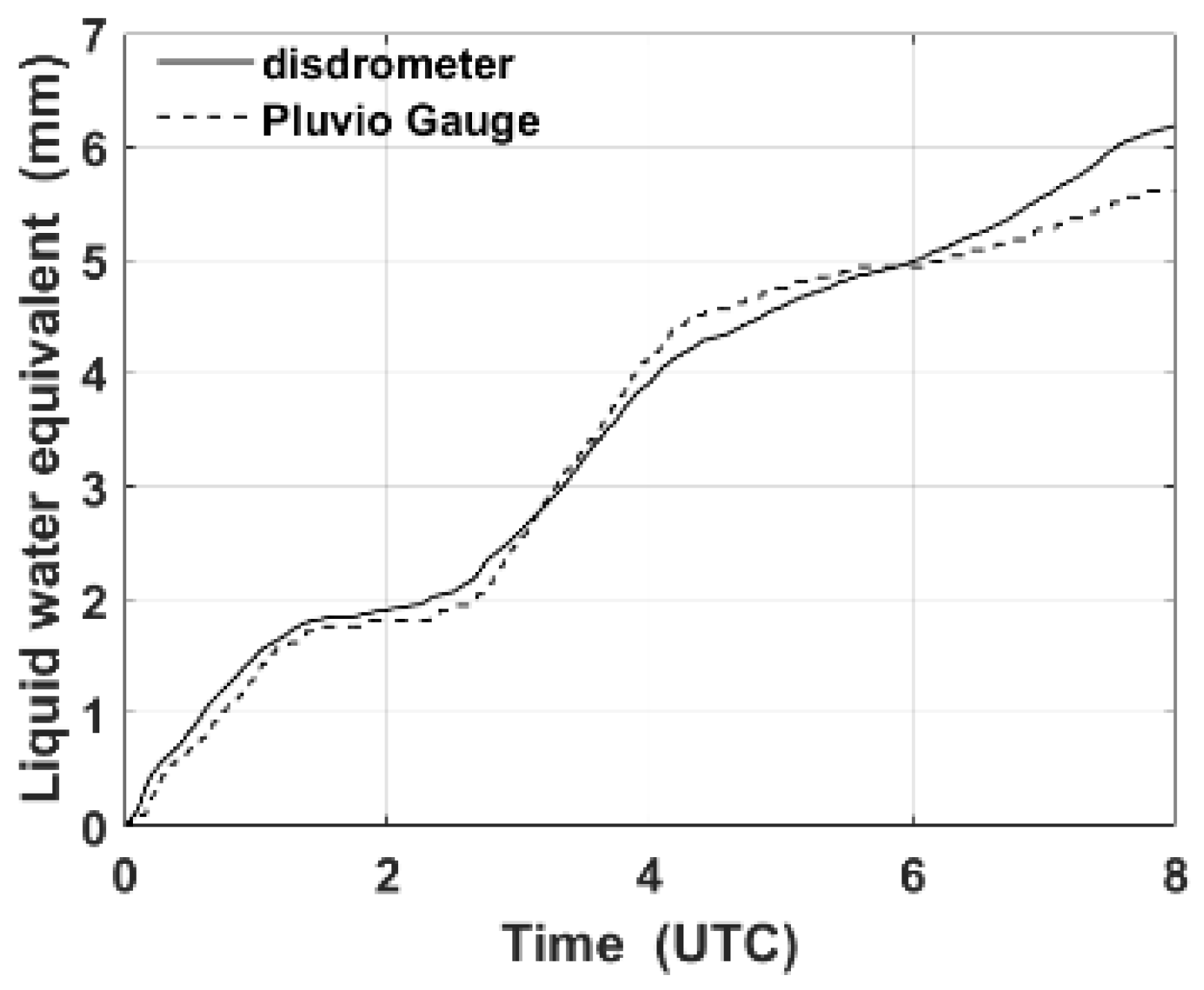
2.1. Instruments and Dataset

In this study, the data was collected by three Parsivel² disdrometers and two PIPs from 2016 to 2018, which includes the period of ICE-POP campaign. The locations of these instruments are illustrated in Figure 1. The Parsivel² disdrometers were deployed at YPO site (37°38′36.03″ N, 128°40′13.78″ E), ODO site (37°50′8.16″ N, 128°38′54.48″ E), and DGW site (37°40′38.39″ N, 128°43′07.77″ E), and PIPs were deployed at MHS site (37°39′54.75″ N, 128°41′58.60″ E) and BKC site (37°44′17.36″ N, 128°48′21.05″ E).

The Parsivel² disdrometer [29,37,38] is a laser-based optical system that produces a horizontal strip of light. The particle size is determined from the reduction of the output voltage when particles pass through the laser beam, and the particle velocity is determined from the duration of the signal. The particle size and velocity are divided into 32 bins varying from 0.062 to 24.5 mm for size and 0.05 to 20.8 m s⁻¹ for velocity. The lowest two size classes (less than 0.312 mm) are eliminated in this study because the signal-to-noise ratio (SNR) is low in these classes.

The Precipitation Imaging Package (PIP) [28,39] is a high-speed camera that records grayscale images of particles at 380 frames per second as they fall over its field of view (64 × 48 mm). These images allow PIP to use this information to extract particle size and velocity. The data quality control for PIP is the same as the Parsivel² disdrometer: if the diameter was less than 0.312 mm then it was not used in this study.

The Pluvio² 200 gauge is used for automatic measurement of the meteorological intensity and amount of precipitation, which has a 200 cm² collecting area and a 1500 mm recording capacity. It determines the weight of precipitation every 6 s with a resolution of 0.01 mm. The gauge is equipped with Tretyakov and Alter Shields [40,41] and placed inside a double-fence intercomparison reference (DFIR) to minimize the effect of wind [41,42,43]. It also uses a special filter algorithm to prevent incorrect measurement [44].

There are two years of measurements (2017–2018) at DGW, MHS, and BKC sites, and three years of measurements (2016–2018) at YPO and ODO sites, and the dataset includes data collected during the PyeongChang 2018 Olympics and Paralympic winter games (ICE-POP 2018) campaign. Precipitation cases, where the temperature was equal to or below 0 °C, were regarded as snow events, while cases that had temperature above 0 °C were not taken into consideration. There are in total 19 snow events in 2016, 19 events in 2017, and 30 snow events in 2018. If data was available, we considered all of the events measurements found at these five sites.

2.2. Snow PSD Parameters

A hydrometeor falling at the terminal velocity can be considered to be a particle moving through a fluid which means the equation of motion is determined from the equilibrium of forces acting on the particle, that is, drag, buoyancy, and gravity. This method is widely used either to retrieve the terminal fall velocity or to retrieve the mass of hydrometeors, and the buoyancy force is ignored because it is too small compared with others [32,45,46,47,48,49,50,51,52,53,54,55]. We use aerodynamic relationships to get the density of snow in this study. Ignoring the buoyancy, inertial forces, and pressure gradient, when gravitational force equals the drag force, the hydrometeor falls relative to the air at its terminal fall speed [56]:

$$\frac{\pi }{4}{D}^2\frac{1}{2}{\rho }_0{v}^2{C}_D=\frac{\pi }{6}{D}^3{\rho }_s$$

(1)

where ${\rho }_0$ is the density of air; v represents the velocity; $C_D$ is the drag coefficient; $g$ is the acceleration of gravity; $D$ represents the diameter observed from Parsivel² disdrometers and PIPs, and it is the equivalent area diameter for PIP and the median volume diameter for Parsivel² disdrometer. The uncertainty of this method is mostly related to observations of the dimensions because some particles are irregular-shaped and observed from a single projection plane perpendicular to the fall direction [51,52]. After getting the velocity and diameter measured from Parsivel² disdrometers and PIPs every minute, the density of snow in every class can be obtained using the relationship below:

$${\rho }_s=\frac{3{\rho }_0{v}^2{C}_D}{4gD}$$

(2)

The volume-weighted mean diameter $D_m$ is computed from measured PSD, denoted by $N\left(D\right)$ in m⁻³ mm⁻¹, where $D$ is the diameter in mm, defined as:

$$D_m=\frac{{{\displaystyle \int }}_0^{D_{max}}{D}^{4}N\left(D\right)dD}{{{\displaystyle \int }}_0^{D_{max}}{D}^{3}N\left(D\right)dD}$$

(3)

Snow PSD is defined as the number of particles in a unit volume for each unit diameter bin, expressed as $\mathrm{N}\left(\mathrm{D}\right)$.

In this study, we used the normalized gamma distribution to describe variations of snow PSD [57]:

$$N\left(D\right)=N_{w}f\left(\mu \right){\left(\frac{D}{D_m}\right)}^{\mu }exp\left(-\lambda D\right)$$

(4)

with

$$f\left(\mu \right)=\frac{6}{4^4}\frac{{\left(4+\mu \right)}^{\mu +4}}{\mathsf{\Gamma }\left(\mu +4\right)}$$

(5)

where $D_m$ is the volume-weighted mean diameter, $\mu$ is the shape factor, $N_w$ is the normalized intercept parameter in units of m⁻³ mm⁻¹ and $N_w$ defined by:

$$N_w=\frac{4^4{{\displaystyle \int }}_0^{D_{max}}{D}^{3}N\left(D\right)dD}{6D_m^4}$$

(6)

The parameter $\mu$ controls the shape of the snow PSD. Estimates of $\mu$ for measured snow PSD can be determined by minimizing the absolute deviation between the normalized gamma form in Equation (4).

Once the snow PSD and the density of snow are known, few integral physics parameters can be calculated, such as ice water content ($IWC$), and liquid water equivalent snowfall rate ($S$). They are expressed as follows:

$$IWC=\frac{\pi }{6}\times {10}^{-3}{{\displaystyle \int }}_0^{D_{max}}{\rho }_s D^{3}N\left(D\right)d$$

(7)

$$S=6\pi \times {10}^{-4}{{\displaystyle \int }}_0^{D_{max}}{\rho }_s D^{3}v\left(D\right)N\left(D\right)d$$

(8)

where $N\left(D\right)$ is in m⁻³ mm⁻¹; $dD$ is in mm; ${\rho }_s$ is the density of snow in g cm⁻³; $v\left(D\right)$ is the terminal fall velocity in m s⁻¹; $D$ is the diameter observed from Parsivel² disdrometers and PIPs measurements; $IWC$ is in g m⁻³; $S$ is in mm h⁻¹. After obtaining the density of snow using Equation (2), snowfall rate and liquid water equivalent snow accumulations can be calculated using Equations (7) and (8).

Figure 2 shows a comparison of liquid water equivalent snow accumulations computed using the density determination based on Parsivel² disdrometer measurements and that were directly measured by Pluvio gauge for 19 March 2018 at YPO site. The meteorological conditions on this date are listed in

Table 1. Meteorological conditions on 19 March 2018. Listed are the times, temperature, humidity, wind speed (here abbreviated as WS), and wind direction (WD).

Time	Temperature (°C)	Humidity (%)	WS (m s−1)	WD (°)
0600 UTC	−0.1	93.0	12.0	81.0
0900UTC	−1.0	97.0	4.6	100.0
1200UTC	−1.1	97.0	9.0	83.0
1500UTC	−1.9	82.0	10.0	81.0

. This is a snow case according to these measurements. The accumulations agree well with the Pluvio gauge after calculating density from measured fall speed and diameters, which indicates the accuracy of the method we used for calculating the density of snow.

3. Results and Discussion

3.1. Distribution of Snow Microphysical Parameters

Figure 3 shows the frequency histograms of snow parameters for all the snowfall events calculated from Parsivel² disdrometers and PIPs. Table 1 shows the statistics of snow parameters: minimum value, median value, mean value, maximum value, standard deviation (STD). From Figure 3 and

Table 2. Statistics of snow PSD parameters for total snowfall events: $\rho$ (g cm⁻³), $lo{g}_{10}IWC$ ($IWC$ in g m⁻³) and $lo{g}_{10}S$ ($S$ in mm h⁻¹)

Parameters	Min	Median	Mean	Max	STD
$\rho$	0.002	0.146	0.211	0.800	0.179
$lo{g}_{10}IWC$	−2.315	−0.904	−0.876	1.054	0.526
$lo{g}_{10}S$	−1.999	−0.3428	−0.3549	2.412	0.741

, it can be observed that the mean value of $\rho$ is 0.146 g cm⁻³ and snow PSD samples with density of 0.05–0.1 g cm⁻³ have the highest frequency, about 24%. The density smaller than 0.2 g cm⁻³ occupies more than 60% and also the frequency of higher density is smaller, which is in agreement with observations of snowfall presented by Tiira et al. [26]. The mean of $lo{g}_{10}IWC$ and $lo{g}_{10}S$ are −0.876 and −0.3549, respectively (mean value of IWC is 0.1330 g m⁻³ and mean value of S is 0.4417 mm h⁻¹), and it is worth noting that snow PSD samples with ice water content less than 0.1330 g m⁻³ and snowfall rate less than 0.4417 mm h⁻¹ account for more than half of total snowfall. The standard deviations of $lo{g}_{10}IWC$ and $lo{g}_{10}S$ (0.526 for $lo{g}_{10}IWC$ and 0.741 for $lo{g}_{10}S$) are large, indicating a high variability of our dataset.

The authors of [33] showed that the relationship between $S$ and $IWC$ follows power-law function. Indeed, estimated values from disdrometer data are in good agreement with fitting a power-law relationship in Figure 4, with $lo{g}_{10}S$ increasing almost linearly with $lo{g}_{10}IWC$, implying that if the IWC is known, the S can be derived. This relationship can be expressed in Equation (9), and the mean difference and correlation coefficient are 0.1149 and 0.9381, respectively. Heymsfield et al. [33] use the relationship between diameter and mass to derive S and IWC and we used Equation (2) to get the density of snow. On the other hand, the S–IWC relationships are different for different pressure levels as indicated in [33], and the relationship proposed in this study is suitable on the ground.

$$S=7.6081\times IW{C}^{1.2626}$$

(9)

Figure 5 shows the scatter plots of $lo{g}_{10}{N}_w$ vs. $D_m$ for all snowfall events. These values are plotted over a wide range, from 0.6 to 6.1 for $lo{g}_{10}{N}_w$ and 0.3 to 19 mm for $D_m$, and the majority of points are within the area of $D_m$ from 0.5 to 6.5 mm and $lo{g}_{10}{N}_w$ from 2.8 to 5.6 for all events.

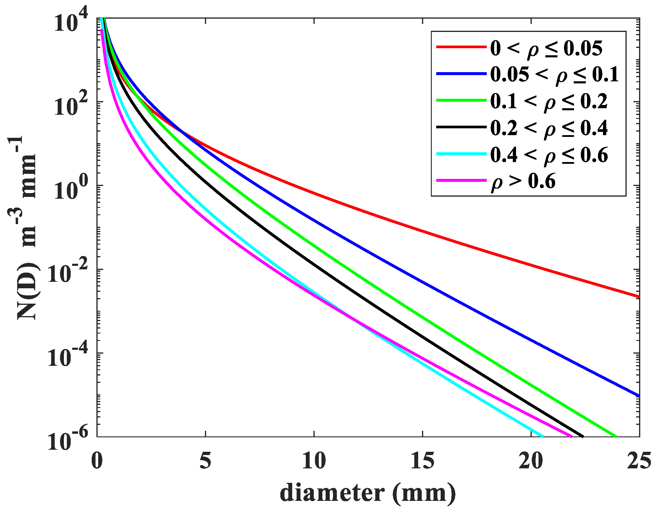
3.2. Snow PSD Characteristics in Different Densities

To further understand the characteristics of snow PSD at different snow densities, we classified the snow density $\rho$ into six classes as follows: 0 < $\rho$≤ 0.05 g cm⁻³, 0.05 < $\rho$ ≤ 0.1 g cm⁻³, 0.1 < $\rho$≤ 0.2 g cm⁻³, 0.2 <$\rho$≤ 0.4 g cm⁻³, 0.4 <$\rho$≤ 0.6 g cm⁻³, and $\rho$> 0.6 g cm⁻³. Figure 6 shows the distribution of $D_m$ and $lo{g}_{10}{N}_w$ for different density classes and the mean values are also indicated. It can be seen that the $D_m$ distribution depends on density and low-density particles are generally larger, this is likely because the particles become more condensed as density increases, thus giving a smaller $D_m$, which is in agreement with previous studies [26,27,28,30,31,32]. This dependence of $D_m$ on density is not surprising, and it is discussed in more detail below. Distributions of $lo{g}_{10}{N}_w$ also exhibit dependence of $lo{g}_{10}{N}_w$ on density because $D_m$ and density are related, dependence of $lo{g}_{10}{N}_w$ on density arises from the dependence on $lo{g}_{10}{N}_w$ on $D_m$, which is the same as previous study [26]. As shown in Figure 6, $lo{g}_{10}{N}_w$ increases with density. The mean values of $D_m$, $lo{g}_{10}{N}_w$, and $\mu$ for different density classes are listed in

Table 3. Mean values of $D_m$, $lo{g}_{10}{N}_w$, and $\mu$ for different density classes.

Density (g cm−3)	No. of Samples	${\mathit{D}}_{\mathit{m}}\mathbf{\left(}\mathbf{mm}\mathbf{\right)}$	$\mathit{l}\mathit{o}{\mathit{g}}_{\mathbf{10}}{\mathit{N}}_{\mathit{w}}$ $\mathbf{\left(}{\mathit{N}}_{\mathit{w}}\mathbf{in}{\mathbf{m}}^{\mathbf{-}\mathbf{3}}{\mathbf{mm}}^{\mathbf{-}\mathbf{1}}\mathbf{\right)}$	$\mathit{\mu }$
0 < $\rho$ ≤ 0.05	7683	4.4961	3.1277	0.6635
0.05 < $\rho$ ≤ 0.1	16,310	2.8786	3.6187	0.4665
0.1 < $\rho$ ≤ 0.2	19,594	2.2275	3.7387	0.4884
0.2 < $\rho$ ≤ 0.4	16,097	1.7091	3.8635	0.9272
0.4 < $\rho$ ≤ 0.6	6799	1.2663	3.9888	1.9253
$\rho$ > 0.6	3894	1.0627	4.0082	3.3837

. From Figure 6 and Table 3, low density events have a broader range of snow PSDs, while high density events demonstrate larger snow particle concentrations. It is clear that $D_m$ decreases with the increasing density, and $lo{g}_{10}{N}_w$ and $\mu$ increase with the increasing density, and these results are consistent with prior studies [26,27,28]. To study the snow PSD shapes of the total categorized data set, Figure 7 shows mean snow PSDs for different density classes. As the density becomes lower, all particle sizes are more frequent which in turn decreases the slope parameter of snow PSDs, which is consistent with previous study [28]. Additionally, the widths of the snow PSDs become broader and show a long tail towards larger diameters. This is because of the composite of a wide range of snow PSDs.

$D_m$ depends on density and there are some size–density relationships that describe the density of snow in previous literature [26,28,30,31,32,53,54,55], and these studies use different methods to obtain the relationships. The first method is that data from a disdrometer is combined with observations from other instruments. The second method uses the general hydrodynamic theory to get the density, and we used this method as mentioned before. However, snow particles vary greatly in different topography and snow event types [26,27,28,30,31,32,33,34,35], so the size-density relationships given in the literature cannot describe the density of snow events captured in the PyeongChang region, as seen the green and magenta lines in Figure 8. Unlike the density of raindrops, the density of snow depends on snowfall types and topography. The complexity of snow density makes snowfall estimation more complex than rainfall estimation. The ice water content is also affected by snow density, so developing a relationship suitable for South Korea is important. Table 2 implies that there are likely different relationships as a function of density ranges and there are different snow microphysics for each range. We categorized the density into three ranges: 0 <$\rho$< 0.1 g cm⁻³, 0.1 <$\rho$≤ 0.2 g cm⁻³, and $\rho$> 0.2 g cm⁻³, and obtained relationships for each range separately. Figure 8 shows the scatter density plot of $\rho$ versus $D_m$ and mean $\rho$-$D_m$ fitting curves for each range. It can be seen that using a piecewise function to describe the relationship between $\rho$ and $D_m$ is more accurate than a relationship in all ranges. We derived a power-law $\rho$-$D_m$ relation using least-squares fitting, which is suitable for the PyeongChang region in South Korea and it can be expressed as:

$$\rho =0.3358D_m^{-1.243}{D}_m>1.7\mathrm{mm}$$

(10)

$$\rho =0.3774D_m^{-1.386}1.7\mathrm{mm}< D_m<2.7\mathrm{mm}$$

(11)

$$\rho =0.462D_m^{-1.879}{D}_m<1.7\mathrm{mm}$$

(12)

Relationships by Brandes et al. [31] and Huang et al. [32] are plotted in Figure 8 for comparison. The density is on average higher for snow events recorded for the PyeongChang region in South Korea. The density of snowfall varies greatly because of different snowfall habits and topography as mentioned in previous studies [26,27,28,30,31,32,33,34,35].

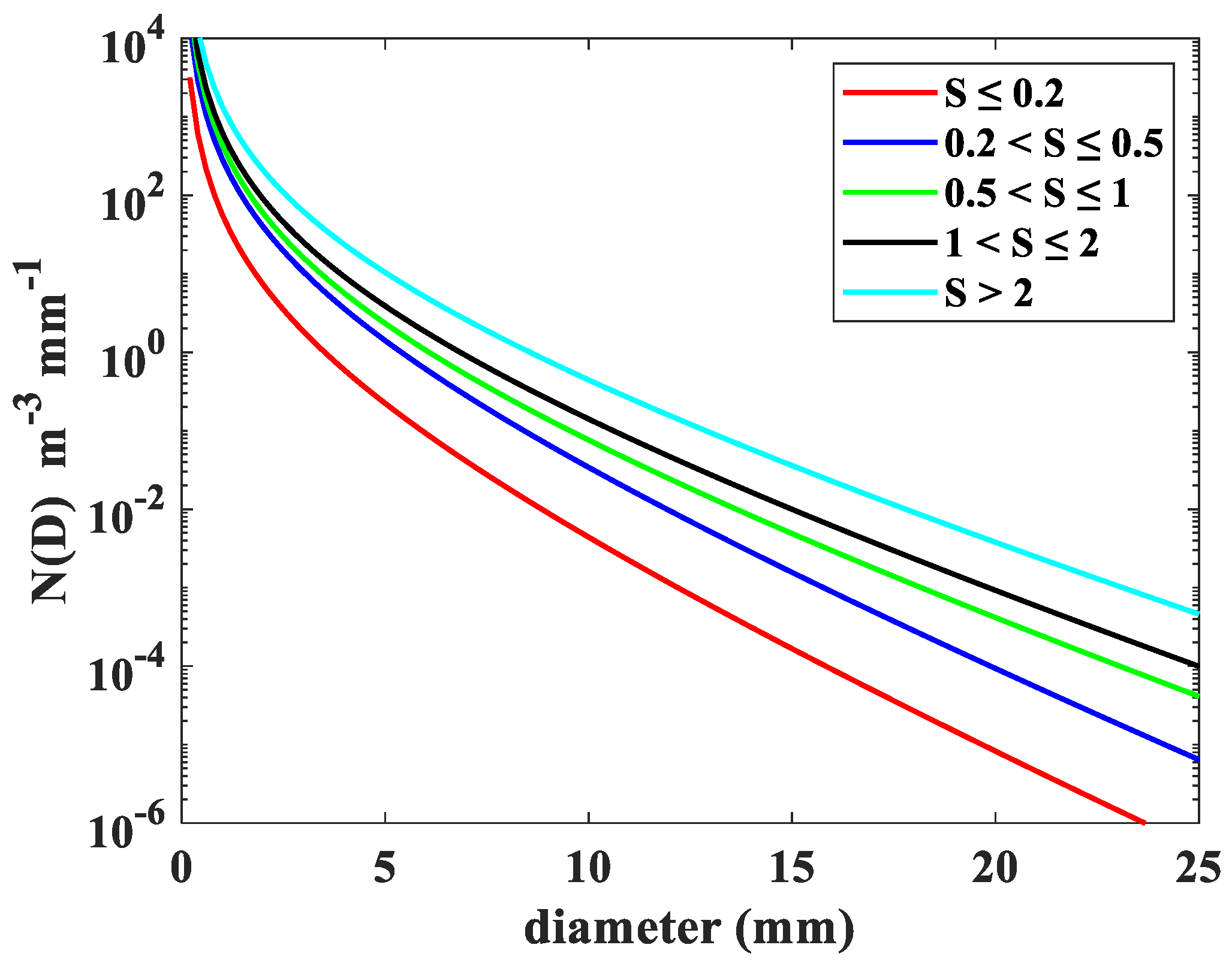
3.3. Snow PSD Characteristics in Different Snowfall Rate Classes

To have a better understanding of the characteristics of snow PSD at different snowfall rate classes, the snow PSD measurements were divided into five classes: S ≤ 0.2 mm h⁻¹, 0.2 < S ≤ 0.5 mm h⁻¹, 0.5 < S ≤ 1.0 mm h⁻¹, 1.0 < S ≤ 2.0 mm h⁻¹, and S > 2 mm h⁻¹. Mean values of $D_m$, $lo{g}_{10}{N}_w$, and $\mu$ for different snow rate classes are listed in

Table 4. Mean values of $D_m$, $lo{g}_{10}{N}_w$, and $\mu$ for different snow rate classes

S (mm h−1)	No. of Samples	${\mathit{D}}_{\mathit{m}}\mathbf{\left(}\mathbf{mm}\mathbf{\right)}$	$\mathit{l}\mathit{o}{\mathit{g}}_{\mathbf{10}}{\mathit{N}}_{\mathit{w}}$ $\mathbf{\left(}{\mathit{N}}_{\mathit{w}}\mathbf{in}{\mathbf{m}}^{\mathbf{-}\mathbf{3}}{\mathbf{mm}}^{\mathbf{-}\mathbf{1}}\mathbf{\right)}$	$\mathit{\mu }$
S ≤ 0.2	11,192	1.3051	3.6499	2.2676
0.2 < S ≤ 0.5	17,458	1.6050	3.7050	1.2885
0.5 < S ≤ 1.0	13,734	1.9254	3.7684	0.7877
1.0 < S ≤ 2.0	11,307	2.1615	3.7661	0.4709
S > 2	16,686	2.7693	3.8013	0.0058

. It is clear that the mean values of $D_m$, $lo{g}_{10}{N}_w$ increase and $\mu$ decreases with the increasing snowfall rate. Figure 9 shows the mean snow PSDs for five snowfall rate classes. The slope of the snow PSDs decreases, and all particle sizes are more frequent with increase of snowfall rate. Furthermore, snow PSDs become broader and the tail of snow PSD shifts gradually to the larger diameter with the increase of snowfall rate, which is in agreement with previous studies [27,34,35].

4. Conclusions

In this paper, three years of observations of snow PSD from three Parsivel² disdrometers and two PIPs deployed at five different sites were analyzed to explore the microphysical characteristics of snowfall in the PyeongChang region of South Korea. Based on these observations, the density of snow ($\rho$), the volume-weighted mean diameter ($D_m$), the normalized intercept parameter ($lo{g}_{10}{N}_w$), ice water content ($lo{g}_{10}IWC$), liquid water equivalent snowfall rates ($lo{g}_{10}S$) were derived. Along with these, the mean fitting normalized gamma distributions for different density classes and snowfall rate classes were also derived. The results of this paper provide a good understanding of the microphysical nature of snowfall, which is useful for remote sensing and NWP and gives a potential use in estimates of snow PSD parameters. The main conclusions are as follows:

1.

For all snowfall events, more than half of the snow PSD measurements are characterized by density less than 0.2 g cm⁻³. The standard deviations of density, ice water content (IWC), and snowfall rate (S) are large which indicates a high variability of particles during the snowfall events. The relationship between snowfall rate and ice water content can be expressed as a power-law function, consistent with the previous study [33]. It implies that if the IWC is known, such as from aircraft measurements, the S can be derived. The pressure level and the way to calculate density can make the relationship different. Additionally, the relationship proposed in this study is suitable for ground observations.

2.

From the results of classified density, the $D_m$ decreases as the density increases, and $lo{g}_{10}{N}_w$ and μ increase as the density increases, PSDs become narrower as the density increases at the same time, and these results are consistent with prior studies [26,28]. $N_w$ and density are related because $D_m$ and density are related, so the dependence of $N_w$ on density is somewhat because of the dependence of $N_w$ on $D_m$ [26].

3.

Stratified by snowfall rate, the snow PSDs become broader as the snowfall rate increases, consistent with previous studies [27,34,35]. Meanwhile, the $D_m$ and $lo{g}_{10}{N}_w$ increase with the increase of snowfall rate and μ decreases with the increase of snowfall rate.

4.

Snow particles vary greatly in different topography and snow events, so the size–density relationships given in the literature might not be suitable for PyeongChang region of South Korea. We used the general hydrodynamic theory in this paper to get the density and the power-law relationship between $\rho$ and $D_m$ for each range and the result is better than previous studies.

The snow PSD measurements at different density classes and snowfall rate classes are represented by normalized gamma distribution and the mean normalized gamma distribution parameters ($N_w$, $D_m$, and $\mu$) were obtained according to different classes. Although this paper presents an understanding of snowfall microphysical variabilities during these three years, future work focused on various other geographical locations is required to further understand the characteristic of snow PSD.

References

1. Mason, B.J. Physics of Clouds and Precipitation. Nat. Cell Biol. 1954, 174, 957–959. [Google Scholar] [CrossRef]
2. Stephens, G.L.; L’Ecuyer, T.; Forbes, R.; Gettelmen, A.; Golaz, J.-C.; Bodas-Salcedo, A.; Suzuki, K.; Gabriel, P.; Haynes, J. Dreary State of Precipitation in Global Models. J. Geophys. Res. Space Phys. 2010, 115. [Google Scholar] [CrossRef]
3. Jakob, C. Accelerating Progress in Global Atmospheric Model Development Through Improved Parameterizations Challenges, Opportunities, and Strategies. Bull. Am. Meteorol. Soc. 2010, 91, 869–875. [Google Scholar] [CrossRef]
4. Tao, W.-K.; Lang, S.; Zeng, X.; Li, X.; Matsui, T.; Mohr, K.; Posselt, D.; Chern, J.; Peters-Lidard, C.; Norris, P.M.; et al. The Goddard Cumulus Ensemble Model (GCE): Improvements and Applications for Studying Precipitation Processes. Atmos. Res. 2014, 143, 392–424. [Google Scholar] [CrossRef] [Green Version]
5. Waliser, D.E.; Li, J.-L.F.; Woods, C.P.; Austin, R.T.; Bacmeister, J.; Chern, J.; Del Genio, A.; Jiang, J.H.; Kuang, Z.; Meng, H.; et al. Cloud Ice: A Climate Model Challenge with Signs and Expectations of Progress. J. Geophys. Res. Space Phys. 2009, 114, 1–27. [Google Scholar] [CrossRef]
6. Bringi, V.N.; Chandrasekar, V.; Hubbert, J.; Gorgucci, E.; Randeu, W.L.; Schoenhuber, M. Raindrop Size Distribution in Different Climatic Regimes from Disdrometer and Dual-Polarized Radar Analysis. J. Atmos. Sci. 2003, 60, 354–365. [Google Scholar] [CrossRef]
7. Dolan, B.; Fuchs, B.; Rutledge, S.A.; Barnes, E.A.; Thompson, E.J. Primary Modes of Global Drop Size Distributions. J. Atmos. Sci. 2018, 75, 1453–1476. [Google Scholar] [CrossRef]
8. Seela, B.K.; Janapati, J.; Lin, P.-L.; Reddy, K.K.; Shirooka, R.; Wang, P.K. A Comparison Study of Summer Season Raindrop Size Distribution Between Palau and Taiwan, Two Islands in Western Pacific. J. Geophys. Res. Atmos. 2017, 122, 11787–11805. [Google Scholar] [CrossRef]
9. Seela, B.K.; Janapati, J.; Lin, P.-L.; Wang, P.K.; Lee, M.-T. Raindrop Size Distribution Characteristics of Summer and Winter Season Rainfall Over North Taiwan. J. Geophys. Res. Atmos. 2018, 123, 11602–11624. [Google Scholar] [CrossRef] [Green Version]
10. Tokay, A.; Short, D.A. Evidence from Tropical Raindrop Spectra of the Origin of Rain from Stratiform versus Convective Clouds. J. Appl. Meteorol. 1996, 35, 355–371. [Google Scholar] [CrossRef] [Green Version]
11. Wen, G.; Xiao, H.; Yang, H.; Bi, Y.; Xu, W. Characteristics of Summer and Winter Precipitation Over Northern China. Atmos. Res. 2017, 197, 390–406. [Google Scholar] [CrossRef]
12. Wen, L.; Zhao, K.; Zhang, G.; Xue, M.; Zhou, B.; Liu, S.; Chen, X. Statistical Characteristics of Raindrop Size Distributions Observed in East China During the Asian Summer Monsoon Season Using 2-D Video Disdrometer and Micro Rain Radar Data. J. Geophys. Res. Atmos. 2016, 121, 2265–2282. [Google Scholar] [CrossRef] [Green Version]
13. Wen, L.; Zhao, K.; Zhang, G.; Liu, S.; Chen, G. Impacts of Instrument Limitations on Estimated Raindrop Size Distribution, Radar Parameters, and Model Microphysics during Mei-Yu Season in East China. J. Atmos. Ocean. Technol. 2017, 34, 1021–1037. [Google Scholar] [CrossRef]
14. Tang, Q.; Xiao, H.; Guo, C.; Feng, L. Characteristics of the Raindrop Size Distributions and Their Retrieved Polarimetric Radar Parameters in Northern and Southern China. Atmos. Res. 2014, 135, 59–75. [Google Scholar] [CrossRef]
15. Thurai, M.; Huang, G.J.; Bringi, V.N.; Randeu, W.L.; Schönhuber, M. Drop Shapes, Model Comparisons, and Calculations of Polarimetric Radar Parameters in Rain. J. Atmos. Ocean. Technol. 2007, 24, 1019–1032. [Google Scholar] [CrossRef]
16. Deo, A.; Walsh, K.J. Contrasting Tropical Cyclone and Non-Tropical Cyclone Related Rainfall Drop Size Distribution at Darwin, Australia. Atmos. Res. 2016, 181, 81–94. [Google Scholar] [CrossRef]
17. Ma, Y.; Ni, G.; Chandra, C.V.; Tian, F.; Chen, H. Statistical Characteristics of Raindrop Size Distribution During Rainy Seasons in the Beijing Urban Area and Implications for Radar Rainfall Estimation. Hydrol. Earth Syst. Sci. 2019, 23, 4153–4170. [Google Scholar] [CrossRef] [Green Version]
18. Chen, B.; Yang, J.; Pu, J. Statistical Characteristics of Raindrop Size Distribution in the Meiyu Season Observed in Eastern China. J. Meteorol. Soc. Jpn. 2013, 91, 215–227. [Google Scholar] [CrossRef] [Green Version]
19. Ji, L.; Chen, B.; Li, L.; Xiao, X.; Zhang, G. Raindrop Size Distributions and Rain Characteristics Observed by a PARSIVEL Disdrometer in Beijing, Northern China. Remote Sens. 2019, 11, 1479. [Google Scholar] [CrossRef] [Green Version]
20. Brandes, E.A.; Zhang, G.; Vivekanandan, J. Experiments in Rainfall Estimation with a Polarimetric Radar in a Subtropical Environment. J. Appl. Meteorol. 2002, 41, 674–685. [Google Scholar] [CrossRef] [Green Version]
21. Chen, H.; Chandrasekar, V.; Bechini, R. An Improved Dual-Polarization Radar Rainfall Algorithm (DROPS2.0): Application in NASA IFloodS Field Campaign. J. Hydrometeorol. 2017, 18, 917–937. [Google Scholar] [CrossRef]
22. Gou, Y.; Ma, Y.; Chen, H.; Wen, Y. Radar- Derived Quantitative Precipitation Estimation in Complex Terrain Over the Eastern Tibetan Plateau. Atmos. Res. 2018, 203, 286–297. [Google Scholar] [CrossRef]
23. Chen, H.; Chandrasekar, V. Estimation of Light Rainfall Using Ku-Band Dual-Polarization Radar. IEEE Trans. Geosci. Remote Sens. 2015, 53, 5197–5208. [Google Scholar] [CrossRef]
24. Cooper, S.J.; Wood, N.B.; L’Ecuyer, T.S. A Variational Technique to Estimate Snowfall Rate from Coincident Radar, Snowflake, and Fall-Speed Observations. Atmos. Meas. Tech. 2017, 10, 2557–2571. [Google Scholar] [CrossRef] [Green Version]
25. Heymsfield, A.J.; Field, P.R.; Bansemer, A. Exponential Size Distributions for Snow. J. Atmos. Sci. 2008, 65, 4017–4031. [Google Scholar] [CrossRef]
26. Tiira, J.; Moisseev, D.; Von Lerber, A.; Ori, D.; Tokay, A.; Bliven, L.F.; Petersen, W. Ensemble Mean Density and Its Connection to Other Microphysical Properties of Falling Snow as Observed in Southern Finland. Atmos. Meas. Tech. 2016, 9, 4825–4841. [Google Scholar] [CrossRef] [Green Version]
27. Pettersen, C.; Kulie, M.S.; Bliven, L.; Merrelli, A.J.; Petersen, W.A.; Wagner, T.J.; Wolff, D.B.; Wood, N.B. A Composite Analysis of Snowfall Modes from Four Winter Seasons in Marquette, Michigan. J. Appl. Meteorol. Clim. 2020, 59, 103–124. [Google Scholar] [CrossRef]
28. Pettersen, C.; Bliven, L.; Von Lerber, A.; Wood, N.B.; Kulie, M.; Mateling, M.E.; Moisseev, D.; Munchak, S.J.; Petersen, W.; Wolff, D.B. The Precipitation Imaging Package: Assessment of Microphysical and Bulk Characteristics of Snow. Atmosphere 2020, 11, 785. [Google Scholar] [CrossRef]
29. Battaglia, A.; Rustemeier, E.; Tokay, A.; Blahak, U.; Simmer, C. PARSIVEL Snow Observations: A Critical Assessment. J. Atmos. Ocean. Technol. 2010, 27, 333–344. [Google Scholar] [CrossRef]
30. Heymsfield, A.J.; Bansemer, A.; Schmitt, C.G.; Twohy, C.; Poellot, M.R. Effective Ice Particle Densities Derived from Aircraft Data. J. Atmos. Sci. 2004, 61, 982–1003. [Google Scholar] [CrossRef]
31. Brandes, E.A.; Ikeda, K.; Zhang, G.; Schönhuber, M.; Rasmussen, R.M. A Statistical and Physical Description of Hydrometeor Distributions in Colorado Snowstorms Using a Video Disdrometer. J. Appl. Meteorol. Clim. 2007, 46, 634–650. [Google Scholar] [CrossRef]
32. Huang, G.-J.; Bringi, V.; Moisseev, D.; Petersen, W.; Bliven, L.; Hudak, D.; Bliven, L. Use of 2D-Video Disdrometer to Derive Mean Density–Size and Ze–SR Relations: Four Snow Cases from the Light Precipitation Validation Experiment. Atmos. Res. 2015, 153, 34–48. [Google Scholar] [CrossRef]
33. Heymsfield, A.J.; Matrosov, S.Y.; Wood, N.B. Toward Improving Ice Water Content and Snow-Rate Retrievals from Radars. Part I: X and W Bands, Emphasizing CloudSat. J. Appl. Meteorol. Clim. 2016, 55, 2063–2090. [Google Scholar] [CrossRef]
34. Braham, R.R. Snow Particle Size Spectra in Lake Effect Snows. J. Appl. Meteorol. 1990, 29, 200–207. [Google Scholar] [CrossRef]
35. Barthold, F.E.; Kristovich, D.A.R. Observations of the Cross-Lake Cloud and Snow Evolution in a Lake-Effect Snow Event. Mon. Weather. Rev. 2011, 139, 2386–2398. [Google Scholar] [CrossRef]
36. ICE-POP. Development Project and Forecast Demonstration; ICE-POP 2018 Science Plan: Daegu, Korea, 2018. [Google Scholar]
37. Kneifel, S.; Von Lerber, A.; Tiira, J.; Moisseev, D.; Kollias, P.; Leinonen, J. Observed Relations Between Snowfall Microphysics and Triple-Frequency Radar Measurements. J. Geophys. Res. Atmos. 2015, 120, 6034–6055. [Google Scholar] [CrossRef] [Green Version]
38. Skofronick-Jackson, G.; Hudak, D.; Petersen, W.; Nesbitt, S.W.; Chandrasekar, V.; Durden, S.; Gleicher, K.J.; Huang, G.-J.; Joe, P.; Kollias, P.; et al. Global Precipitation Measurement Cold Season Precipitation Experiment (GCPEX): For Measurement’s Sake, Let It Snow. Bull. Am. Meteorol. Soc. 2015, 96, 1719–1741. [Google Scholar] [CrossRef]
39. Newman, A.J.; Kucera, P.A.; Bliven, L.F. Presenting the Snowflake Video Imager (SVI). J. Atmos. Ocean. Technol. 2009, 26, 167–179. [Google Scholar] [CrossRef]
40. Lanza, L.; Leroy, M.; Alexandropoulos, C.; Stagi, L.; Wauben, W. Instruments and Observing Methods. Report No. 84. WMO Laboratory Intercomparison of Rainfall Intensity Gauges; WMO/TD-No. 1304; WMO: Geneva, Switzerland, 2006. [Google Scholar]
41. Rasmussen, R.; Baker, B.; Kochendorfer, J.; Meyers, T.; Landolt, S.; Fischer, A.P.; Black, J.; Thériault, J.M.; Kucera, P.; Gochis, D.; et al. How Well Are We Measuring Snow: The NOAA/FAA/NCAR Winter Precipitation Test Bed. Bull. Am. Meteorol. Soc. 2012, 93, 811–829. [Google Scholar] [CrossRef] [Green Version]
42. Kochendorfer, J.; Rasmussen, R.; Wolff, M.; Baker, B.; Hall, M.E.; Meyers, T.; Landolt, S.; Jachcik, A.; Isaksen, K.; Brækkan, R.; et al. The Quantification and Correction of Wind-Induced Precipitation Measurement Errors. Hydrol. Earth Syst. Sci. 2017, 21, 1973–1989. [Google Scholar] [CrossRef] [Green Version]
43. Wolff, M.A.; Isaksen, K.; Petersen-Øverleir, A.; Ødemark, K.; Reitan, T.; Brækkan, R. Derivation of a New Continuous Adjustment Function for Correcting Wind-Induced Loss of Solid Precipitation: Results of a Norwegian Field Study. Hydrol. Earth Syst. Sci. 2015, 19, 951–967. [Google Scholar] [CrossRef]
44. OTT. Operating Instructions Precipitation Gauge OTT Pluvio2 L; OTT Hydromet Gmbh: Kempten, Germany, 2012. [Google Scholar]
45. Mitchell, D.L. Use of Mass-and Area-Dimensional Power Laws for Determining Precipitation Particle Terminal Velocities. J. Atmos. Sci. 1996, 53, 1710–1723. [Google Scholar] [CrossRef]
46. Hanesch, M. Fall Velocity and Shape of Snowflakes. Ph.D. Thesis, Swiss Federal Institute of Technology, Zurich, Switzerland, 1999; p. 123. [Google Scholar]
47. Khvorostyanov, V.I.; Curry, J.A. Terminal Velocities of Droplets and Crystals: Power Laws with Continuous Parameters over the Size Spectrum. J. Atmos. Sci. 2002, 59, 1872–1884. [Google Scholar] [CrossRef]
48. Khvorostyanov, V.I.; Curry, J.A. Fall Velocities of Hydrometeors in the Atmosphere: Refinements to a Continuous Analytical Power Law. J. Atmos. Sci. 2005, 62, 4343–4357. [Google Scholar] [CrossRef]
49. Mitchell, D.L.; Heymsfield, A.J. Refinements in the Treatment of Ice Particle Terminal Velocities, Highlighting Aggregates. J. Atmos. Sci. 2005, 62, 1637–1644. [Google Scholar] [CrossRef]
50. Heymsfield, A.J.; Westbrook, C.D. Advances in the Estimation of Ice Particle Fall Speeds Using Laboratory and Field Measurements. J. Atmos. Sci. 2010, 67, 2469–2482. [Google Scholar] [CrossRef] [Green Version]
51. Szyrmer, W.; Zawadzki, I. Snow Studies. Part II: Average Relationship between Mass of Snowflakes and Their Terminal Fall Velocity. J. Atmos. Sci. 2010, 67, 3319–3335. [Google Scholar] [CrossRef] [Green Version]
52. Wood, N.B.; L’ecuyer, T.S.; Bliven, F.L.; Stephens, G.L. Characterization of Video Disdrometer Uncertainties and Impacts on Estimates of Snowfall Rate and Radar Reflectivity. Atmos. Meas. Tech. 2013, 6, 3635–3648. [Google Scholar] [CrossRef] [Green Version]
53. Wood, N.B.; L’Ecuyer, T.S.; Heymsfield, A.J.; Stephens, G.L.; Hudak, D.R.; Rodriguez, P. Estimating Snow Microphysical Properties Using Collocated Multisensor Observations. J. Geophys. Res. Atmos. 2014, 119, 8941–8961. [Google Scholar] [CrossRef]
54. Szyrmer, W.; Zawadzki, I. Snow Studies. Part III: Theoretical Derivations for the Ensemble Retrieval of Snow Microphysics from Dual-Wavelength Vertically Pointing Radars. J. Atmos. Sci. 2014, 71, 1158–1170. [Google Scholar] [CrossRef]
55. von Lerber, A.; Moisseev, D.; Bliven, L.F.; Petersen, W.; Harri, A.M.; Chandrasekar, V. Microphysical Properties of Snow and Their Link to Z E–S Relations During BAECC 2014. J. Appl. Meteorol. Climatol. 2017, 56, 1561–1582. [Google Scholar] [CrossRef]
56. Rogers, R.R.; Mason, B.J.; Sartor, J.D. A Short Course in Cloud Physics, 3rd ed.; Butterworth-Heinemann: Oxford, UK, 1989. [Google Scholar]
57. Bringi, V.N.; Chandrasekar, V. Polarimetric Doppler Weather Radar: Principles and Applications; Cambridge University Press (CUP): Cambridge, UK, 2001. [Google Scholar]
Figure 1. The locations of Parsivel2 disdrometers and Precipitation Imaging Package (PIP) used during ICE-POP 2018 in this study. Parsivel2 disdrometers were located at YPO, ODO, and DGW sites, and PIPs were located at MHS and BKC sites.
Atmosphere 11 01093 g001
Figure 2. Comparison of liquid water equivalent snow accumulations computed using the density determination based on Parsivel2 disdrometer measurements (Equation (2)) and that were directly measured by Pluvio2 gauge for 19 March 2018 at YPO site.
Atmosphere 11 01093 g002
Figure 3. Histograms of snow PSD parameters for total snowfall events: (a) the density of snow, ρ (g cm−3); (b) ice water content,   l o g 10 I W C ( I W C in g m−3); (c) liquid water equivalent snowfall rates, l o g 10 S ( S in mm h−1).
Atmosphere 11 01093 g003
Figure 4. Scatter density plot of S and I W C . The black line is the fitting curve.
Atmosphere 11 01093 g004
Figure 5. Scatter density plot of l o g 10 N w versus D m for all snowfall events.
Atmosphere 11 01093 g005
Figure 6. Histograms of D m and l o g 10 N w for different density classes: (a) 0 <   ρ   ≤ 0.05 g cm3, (b) 0.05 <   ρ   ≤ 0.1 g cm−3, (c) 0.1 <   ρ   ≤ 0.2 g cm−3, (d) 0.2 <   ρ   ≤ 0.4 g cm3, (e) 0.4 <   ρ   ≤ 0.6 g cm−3, (f) ρ   > 0.6 g cm−3.
Atmosphere 11 01093 g006aAtmosphere 11 01093 g006b
Figure 7. Mean snow PSDs for six density classes: 0 <   ρ   ≤ 0.05 g cm−3, 0.05 <   ρ   ≤ 0.1 g cm−3, 0.1 <   ρ   ≤ 0.2 g cm−3, 0.2 <   ρ   ≤ 0.4 g cm−3, 0.4 <   ρ   ≤ 0.6 g cm−3, and ρ   > 0.6 g cm−3.
Atmosphere 11 01093 g007
Figure 8. Scatter density plot for ρ (g cm−3) versus D m (mm) and mean ρ - D m power-law fitting for different ranges. Black fitting is for ρ   > 0.2, red fitting is for 0.1 <   ρ   < 0.2, and blue fitting curve is for 0 < ρ   < 0.1.
Atmosphere 11 01093 g008
Figure 9. Mean snow PSDs for six density classes: S ≤ 0.2 mm h−1, 0.2 < S ≤ 0.5 mm h−1, 0.5 < S ≤ 1.0 mm h−1, 1.0 < S ≤ 2.0 mm h−1, and S > 2 mm h−1.
Atmosphere 11 01093 g009