Article

Differentiating Snow and Glacier Melt Contribution to Runoff in the Gilgit River Basin via Degree-Day Modelling Approach

1
Key Laboratory of Tibetan Environment Changes and Land Surface Processes, Institute of Tibetan Plateau Research, Chinese Academy of Sciences, Beijing 100101, China
2
CAS Center for Excellence in Tibetan Plateau Earth Sciences, Chinese Academy of Sciences, Beijing 100101, China
3
Institute of International Rivers and Eco-Security, Yunnan University, Kunming 650500, China
4
International Centre for Integrated Mountain Development, GPO Box 3226, Khumaltar, Kathmandu 44600, Nepal
5
State Key Laboratory of Cryospheric Science, Northwest Institute of Eco-Environment and Resources, Chinese Academy of Sciences (CAS), Lanzhou 730000, China
6
Centre for Integrated Mountain Research, University of the Punjab, Lahore 54000, Pakistan
7
ICARUS/Department of Geography, Maynooth University, W23 F2K8 Maynooth, Ireland
*
Author to whom correspondence should be addressed.
Atmosphere 2020, 11(10), 1023; https://doi.org/10.3390/atmos11101023
Submission received: 22 July 2020 / Revised: 9 September 2020 / Accepted: 16 September 2020 / Published: 23 September 2020
(This article belongs to the Section Meteorology)

Abstract

:
In contrast to widespread glacier retreat evidenced globally, glaciers in the Karakoram region have exhibited positive mass balances and general glacier stability over the past decade. Snow and glacier meltwater from the Karakoram and the western Himalayas, which supplies the Indus River Basin, provide an essential source of water to more than 215 million people, either directly, as potable water, or indirectly, through hydroelectric generation and irrigation for crops. This study focuses on water resources in the Upper Indus Basin (UIB) which combines the ranges of the Hindukush, Karakoram and Himalaya (HKH). Specifically, we focus on the Gilgit River Basin (GRB) to inform more sustainable water use policy at the sub-basin scale. We employ two degree-day approaches, the Spatial Processes in Hydrology (SPHY) and Snowmelt Runoff Model (SRM), to simulate runoff in the GRB during 2001–2012. The performance of SRM was poor during July and August, the period when glacier melt contribution typically dominates runoff. Consequently, SPHY outperformed SRM, likely attributable to SPHY’s ability to discriminate between glacier, snow, and rainfall contributions to runoff during the ablation period. The average simulated runoff revealed the prevalent snowmelt contribution as 62%, followed by the glacier melt 28% and rainfall 10% in GRB. We also assessed the potential impact of climate change on future water resources, based on two Representative Concentration Pathways (RCP) (RCP 4.5 and RCP 8.5). We estimate that summer flows are projected to increase by between 5.6% and 19.8% due to increased temperatures of between 0.7 and 2.6 °C over the period 2039–2070. If realized, increased summer flows in the region could prove beneficial for a range of sectors, but only over the short to medium term and if not associated with extreme events. Long-term projections indicate declining water resources in the region in terms of snow and glacier melt.

Graphical Abstract

1. Introduction

The Upper Indus Basin (UIB) combines the high mountain ranges of the Hindukush, Karakoram, and Himalaya (HKH) [1]. Snow and glacier meltwater from this region is the main contributor to 10 major river basins downstream. Water resources from the region directly or indirectly sustain the livelihoods of 215 million people through the provision of water for agriculture, human consumption, and hydroelectricity generation [2,3]. The UIB has the most extensive glacier coverage of High Mountain Asia (HMA) [4] and contributes the largest amount of seasonal snowmelt of all Asian river basins [5,6]; the Indus basin exhibits the second highest melt contribution from snow on ice after the Brahmaputra Basin amongst other basins in HMA [3]. In contrast, the large rivers of Southeast and South Asia are largely dependent on summer monsoonal wet regimes.
Consistent with the observed global reduction in glacier ice and snow volume [7], recent cryospheric studies in the HKH region have found general glacier retreat [8]. Noticeably, the glaciers in the eastern and central HKH region are rapidly losing mass and exhibit negative mass balances with shrinkage rates similar to those reported elsewhere [9]. In contrast, the Karakoram region has exhibited positive mass balances and glacier stability over the last decade [10,11,12]. Fluctuations in glacier mass balance and consequent alterations in glacier/snowmelt contribution to runoff can lead to an increased prevalence of floods or droughts. If future projections of climate change for the region are realized, alterations in seasonal streamflow, due to changes in glacier mass balance and snow accumulation, may present significant new opportunities and challenges for water resource management in the region. Even in the absence of climate change, projected increases in population in the region will place additional pressures on already vulnerable water and energy supplies. Moreover, extreme weather events are also likely to become more frequent in the future which pose serious threats to a region which is already experiencing severe flooding events and other natural hazards.
The Indus River is measured at ten primary gauges including its tributaries, namely the Astore, Gilgit, Hunza, Shigar, and Shyok basins. Due to the diversity in the hydrological regimes linked with snow and glaciers, these basins are typically classified on the basis of their correlation with particular climatic variables [13]. Previous studies partitioned the snow/glacier-fed regions of UIB based on the area of glacier coverage and a correlation between runoff and winter precipitation, obtained from low altitude stations [14,15]. On this basis, the Astore and Gilgit sub-basins are classified as snow- dominated basins, while the Shigar and Shyok sub-basins are classified as glacier-dominated basins. Previous studies have simulated daily runoff for the snow and glacier regions using different hydrological models, including models with snow components [16,17,18]. The Snowmelt Runoff Model (SRM) was applied in high altitude regions to simulate, and subsequently forecast, daily stream flows [19,20]. On the basis of previous studies, it is estimated that the UIB contributes approximately 65% of the annual river flow, with meltwater mainly derived from the seasonal, permanent, and glaciated areas above 3500 m in elevation [21]. The ability of this region to supply water is dependent on the accumulation of snow during October–March and the temperature at high altitude during the ablation period, from April to September [13,14].
Evidence of changing climate impacts on the hydrologic response of the UIB has also been found, using both observational and model-based approaches [1,22]. However, a number of limitations have been highlighted, associated with precipitation underestimation and bias calibration methods, which have curtailed the development of policy to inform more sustainable water resources management in the region [23]. Studies have also highlighted the lack of spatiotemporal data coverage and quality of datasets employed, which impact the variability in simulations and uncertainty in estimating snowmelt contribution to runoff. Previous hydrological modelling studies within UIB [1,24,25], assessing the impact of climate variability on projected future flows, found significant biases in runoff contribution which they attributed to the selection of large catchment areas, poor quality/sparse precipitation data, and choice of Degree Day Factor (DDF) and/or temperature lapse rate (TLR) [23]. More recent studies have sought to address these shortcomings by employing more specific DDF and TLR applied at sub-basin scales [3,26,27,28,29].
A number of studies [25,27,28] have employed the Snowmelt Runoff Model (SRM), which was designed for runoff simulation in snow dominant basins. However, when this model is used in a partly glacier-fed basin resulting in the neglection of the glacier-melt contribution, model accuracy can be compromised. SRM was previously employed in the Astore, Gilgit, and Hunza sub-basins [24,25,28] and was found to produce reliable outputs for these three basins, but results were presented without considering the glacier melt contribution to runoff. The Astore and Hunza sub-basins range from 1504 to 8069 and 1420 to 7809 m.a.s.l. with around 14% and 28% of the total area, respectively covered by glaciers and permanent ice cover [13,30]. Importantly, it may also be necessary to consider that glacier cover melt-rates vary depending on whether a glacier consideration is debris-covered or clean-ice [31,32,33]. Similarly, the most recent studies based on snow cover assessment and hydrological modelling were carried out in the Gilgit River Basin (GRB) and neighboring river basins [27,28,29,34]. These studies focused on the climatic and snow cover trends for both the present and future, without considering glacier coverage (clean ice/debris-covered) [35] for the selected basins. Alternatively, [27] classified clean and debris-covered ice and employed the Modified Positive Degree Day Modelling (MPDDM) approach to address snow and ice contributions in GRB, rather than including the precise glacier melt contribution to flow. While a number of studies addressed the contribution of glaciers in terms of melting from snow on land (SOL), snow on ice (SOI), and exposed glaciers ice (EGI) [3], results were based on the melting rate generated by clean-ice glaciers rather than including the precise debris-covered glacier fraction. Over the period 2001 to 2012, the GRB had between 15–80% snow-covered areas, with 8% covered by glacier ice [13]. According to recent estimates [27], around 1139 km2 of the total 12,655 km2 area is glacier-covered (around 9%). Despite representing a relatively small percentage of the total area, the glacier coverage contribution to snowmelt runoff should be taken into account in order to calculate more reliable runoff estimates, particularly in the context of any future changes in climate in the region. SRM has been shown to be an appropriate and widely used tool for snowmelt runoff simulation and can be used for differentiating snow and glacier melt; however, the user needs to execute the model separately for both snow and glaciers. Alternatively, the Spatial Processes in Hydrology (SPHY) model, which uses a degree-day approach [36] for simulating snowmelt and glacier melt concurrently, has also been employed in the UIB [37]. When employed with gridded datasets as input, SPHY was found to reliably simulate the flows generated by snow and glacier meltwater at the measuring outlet, after classifying all the clean-ice and debris-covered glacier fractions.
Here, we generate runoff simulations within the Gilgit basin using both SRM and SPHY, for the period 2001 to 2012. The present study seeks to build on previous work by employing available observed data within GRB and covering an elevation range from 1480 (Gilgit) to 3280 m.a.s.l (Yasin). Moreover, we use a state-of-the-art degree-day modelling approach, namely SPHY, to represent glacier melt contributions from both clean-ice and debris-covered glaciers within the GRB. The core objective of the work is to understand the effect of temperature and precipitation on the fluctuation of streamflow in the region, flows being highly sensitive to precipitation and temperature in the form of direct (precipitation), delayed (snowmelt) and glacier runoff. We incorporated the Moderate Resolution Imaging Spectroradiometer (MODIS) snow cover products (MOD10A2 8-day maximum composite), an essential requirement for input to SRM. The present study also investigates potential future changes in runoff due to climate change, specifically concerning temperature, precipitation, and streamflow and both temporally and spatially within GRB. We also derived a basin-wide glacier fraction map based on debris-covered and clean-ice glaciers. We present the combination of two degree-day modelling approaches for the first time within GRB. It is intended that the findings will directly inform the development of more sustainable water use policies, in the context of a changing climate, and improved water resources management.

2. Data and Methods

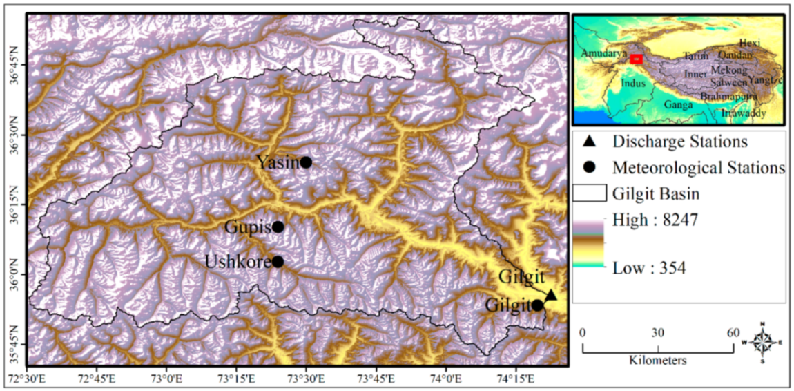
2.1. Study Region Description

The Gilgit basin is a sub-basin of UIB and encompasses the region from 35.8–37° N to 72.5–74.4° E, including the eastern part of the Hindukush range. The drainage area of this basin incorporates 12,000 km2 with an elevation range of 1481–7134 m.a.s.l, as shown in Figure 1. The primary controls on precipitation in the basin are associated with disturbances in the upper-level westerlies and the summer monsoon [13]. The basin has approximately 685 glaciers and 605 glacial lakes. Eight of these lakes have been identified as a potential threat due to Glacial Lake Outburst Floods (GLOF) [27]. The careful selection of GRB involves its cryospheric extent based on snow and glacier coverage. Dominant snow coverage makes this basin perfect for using SRM, while slight glacier coverage in terms of clean-ice and debris-covered glaciers ensure smooth application of SPHY.

2.2. Data

2.2.1. Hydro-Climatological Data

Three organizations, the Pakistan Meteorological Department (PMD), the Surface Water Hydrology Project Water and Power Development Authority (SWHP-WAPDA), and the Snow and Ice Hydrology Project (SIHP-WAPDA), are responsible for the network of meteorological and hydrological stations installed within Pakistan’s territory [38]. World Meteorological Organization (WMO) guidelines are followed for the installation of instrumentation, data acquisition, and subsequent distribution of data to users [39]. The PMD operates six manual valley-based stations, including Gilgit (1460 m.a.s.l) and Gupis (2156 m.a.s.l) and data for these stations are available from the 1960s onwards. The streamflow network is primarily managed by SWHP-WAPDA. High altitude data collection is operated by SIHP-WAPDA, which consists of 12 high altitude Automatic Weather Stations (AWS) including Ushkore (3051 m.a.s.l) and Yasin (3280 m.a.s.l) [13,40]. Daily hydroclimatic data (e.g., precipitation, temperature, and flows) at all four stations, including a streamflow gauge on Gilgit River at Gilgit (Figure 1), were provided by the PMD and WAPDA.

2.2.2. Meteorological and Climate Model Data

The SRM and SPHY models use daily temperature and precipitation data to simulate runoff. The required meteorological data are available from Future Water, for the Hindukush–Himalayan Region, as shown in Table 1. These meteorological data are derived from the Watch Forcing Data ERA-INTERIM (WFDEI). We subsequently converted the available daily Tmax, Tmin, Tavg, and precipitation (Prec) data into the required format for input into SPHY and SRM.
We employed global daily downscaled data (GDDP) for the assessment of climate flows due to a changing climate. This dataset is provided for assessing climate change impacts at local to regional scales and to enhance public understanding of possible future climate patterns at the spatial scale of individual towns, cities, and watersheds. The GDDP dataset contains downscaled climate scenarios for the globe derived from General Circulation Model (GCM) runs conducted as part of the Coupled Model Intercomparison Project Phase 5 (CMIP5) [41]. These datasets provide two of four greenhouse gas emissions scenarios, referred to as Representative Concentration Pathways (RCPs), namely RCP 4.5 and RCP 8.5 [42]. The CMIP5 GCM simulations were undertaken in support of the Intergovernmental Panel on Climate Change’s (IPCC) Fifth Assessment Report (FAR) [43]. A number of limitations exist with the use of these data. Firstly, regional or local climate analyses typically require detailed spatial and temporal climate information, and consequently, the coarse grid resolution may act to smooth some of the local climate variability. Secondly, global projections, particularly at the regional scale, display (systematic) biases which need to be accounted for before use [44].
While recognizing these shortcomings, we employed climate data from the Can-ESM2 and Nor-ESM1-M Global Climate Models (GCMs), based on RCP 4.5 and 8.5, for use in SRM within GRB, to assess the potential impact of climate change on future river flows in the region. The NEX-GDDP datasets are generated by the Bias-Correction Spatial Disaggregation (BCSD) method featuring a statistical downscaling approach to address limitations of directly employing GCM output [45,46,47]. The bias correction method employs spatial details acquired from observational datasets for the interpolation of GCM outputs to higher resolution grids. The algorithms compare GCM output with observed climate data for a common or overlap period; the difference is then used to statistically ‘bias correct’ or adjust the climate model projections based on the assumption that any differences are systematic. The downscaled datasets generated by BCSD also assume that the relative spatial patterns in precipitation and temperature during the historical period will remain constant under the future climate change scenarios—referred to as pattern scaling. The relative spatial patterns are then used to disaggregate the bias-corrected climate model data to the same grid resolution as the observations, using a bilinear interpolation technique. The spatial details of fine-grained observations are preserved using this technique, for example, by computing observed daily precipitation values which are multiplied by a scaling factor to adjust the daily interpolated GCM projections to produce pattern scaled, regional/local climate projections [48].

2.2.3. Ancillary/Satellite Derived Data

SRM requires snow cover products as a primary input; due to the scarcity of available in situ data, remotely sensed data are typically utilized [20]. MODIS 8 days L3 Global 500 m grid processed snow cover products (MOD10A2) were used to calculate the extent of snow cover area during 2000–2018 within the GRB. We processed 430 available images, from April 2000 to September 2018, using the maximum extent of snow cover spanning the 8-day coverage to minimalize error due to cloud cover. The selected images were subsequently mosaicked and projected using ENVI + IDL 4.7; the images for the Gilgit basin were then extracted from these mosaicked scenes. Finally, we calculated the snow cover area (SCA) for seven different altitudinal zones within GRB. However, the lower albedo prevents the MODIS platform from acquiring precise debris-covered glacier fractions.
Daily forcing data are available from the SPHY database for the Hindukush–Himalayan region; alternatively, user-defined data can be employed. In this study, we employed a higher resolution digital elevation model (DEM) derived from NASA’s Shuttle Radar Topography Mission (SRTM) obtained at 90 m resolution. All user-defined datasets were subsequently converted to comma delimited (e.g., CSV) format using the method outlined in the SPHY manual. We used similar CSV formatted files for the basic meteorological forcing for the stations outlined in Table 1.

2.3. Methods

2.3.1. Snowmelt Runoff Model (SRM)

SRM is a conceptual, deterministic degree-day model used to simulate daily streamflow values resulting from snowmelt and precipitation in mountainous regions. The basic inputs for the SRM are daily temperature, precipitation, and SCA.
Streamflow is calculated as
Q n + 1 = [ C sn ·   a n + ( T n + Δ T n )   C Rn   P n ]   A . 1000 86400   ( 1 K n + 1 ) + Q n   K n + 1
where Q n + 1 is the discharge at day n+1 (m3/s); C sn is the snow runoff coefficient; a n is the degree-day factor on day n (cm/°C/day); T n + Δ T n are the degree days (°C); S n is the fractional snow cover; C Rn is the rain runoff factor; P n is the rain on day n (cm); A is total area(km2); K n + 1 is discharge recession coefficient. An illustration of the methodology is shown in Figure 2.
A detailed description of the SRM model is provided by [20]. The SRM is more sensitive to snow cover data as compared to precipitation data. Therefore, it is preferable to use snow cover data, when available precipitation data are sparse or less reliable [24]. Furthermore, SRM is unable to calculate glacier area coverage by default; an assumption is made that the glacier extent is persistent for the calculation of actual contribution from glaciers for debris-covered as well as clean-ice glaciers. This is based on the fact that glacier area changes occur over longer durations as compared to the seasonal snow cover which melts seasonally. Another limitation of the model is introduced at the basin scale, where the use of a single DDF value is assumed to be representative of the entire basin and for both debris-covered and clean-ice glacier fractions. An alternative approach involves the spatial disaggregation of the basin into representative zones (zone-wise application), depending upon the basin size [49]. Here, we used SRM in zone-wise application by extracting seven altitudinal zones from the entire GRB (Figure 3). We divided the basin zones using a DEM and subsequently calculated the SCA for each zone. The study area of GRB calculated by SPHY was around 12,300 km2 which is approximately equal to the area calculated using the DEM. The zones are outlined in Table 2.
An overview of the parameters and calibrated values for SRM is provided in Table 3. TLR is considered as the most sensitive parameter in the temperature-based/degree-day modelling approach. Previous studies [50] reported that underestimation of the TLR may lead to an underestimation of melting rates and vice versa. TLR typically varies between −0.98 to 0 °C/100 m, referred to as dry adiabatic and isothermal lapse rate, respectively, and the global standard lapse rate of −0.65 °C/100 m is widely used [51]. Previous studies within high altitude areas [24,52,53] have employed annual TLR values ranging from −0.2 to −0.9 °C/100 m in model simulations. We used station data up to 3280 m (Yasin) as the temperature input for model runs. We extrapolated the temperature values above this elevation range in different altitudinal zones using a lapse rate ranging from −0.42 to −0.59 °C/100 m for various zones. Previously, [24,28] used −0.48 to −0.76 and −0.64 °C/100 within the Hunza and Gilgit basins, respectively, which is slightly higher than the values used in adjacent regions such as the Tibetan Plateau (TP) [26]. The authors also proposed that the constant value of TLR does not accord with the environmental conditions experienced in the TP and adjoining regions. Consequently, we employed a TLR value ranges −0.42 to −0.53 °C/100 m, suggested by [54], which is closer to the average global TLR.
The melting rates for clean ice and snow vary over UIB. According to [55], the melt rate is 0.7 and 0.4 cm/°C/day for clean ice and snow, respectively. Previous studies reported differences in DDF with regards to elevation, while [47] reported a depressed DDF attributed to a lower value associated with the density of fresh snow. Some authors [24] used 0.5 to 0.7 cm/°C/day for zone-wise application, however, [28] used 0.1 to 0.6 cm/°C/day during early to late ablation period. Some authors [26] have employed a constant DDF value for snow and glacier ice for the TP. They also reported that variations in DDF result in an overestimation of new snow, resulting in faster snowmelt in the model simulation. These authors suggested the use of a varying DDF based on season and elevation zones. Here, we employ a varying DDF for each month, from April to September i.e., 0.5 for April-May, 0.75 for June-August and 0.35 cm/°C/d for September. These values were calibrated based on geodetic mass balance data for snow, clean-ice and debris-covered glaciers in the Karakoram region [37]. The GRB is a snow dominant basin, therefore DDF is lower in the beginning but increases during peak ablation period for melting of the snow and the clean-ice glacier. However, it decreases in September when melt contribution generates by the debris-covered glacier. This value can be opted out depending upon the glacier extent (clean-ice/debris-covered) for rest of the basins in UIB. We also used the varying value for Rainfall contributed area (RCA) as ‘1′ for June-August and ‘0′ for May and September. The duration of the period concerned was April to September i.e., snowmelt/glacier melt period. It is assumed that when rain falls on previous snow cover, an equal amount of water will be released from the snowpack so that the rain from that area could be added as snowmelt [56]. The melting effect of the rain was neglected due to the small amount of additional heat supplied by the liquid precipitation [57], ultimately a pragmatic simplification. Some other parameters such as rainfall (Cs) and snow (Cr) runoff coefficients which dictate the conversion of rainfall and snowfall into the runoff. Similarly, recession coefficients (Xc and Yc) account for the runoff contribution by snowmelt occurred on the previous day. These parameters were calibrated according to previous studies as suggested by [28]. Calibration parameter values for the zone-wise application of SRM are given in Table 3.

2.3.2. Spatial Processes in Hydrology (SPHY)

The SPHY is a spatially distributed, leaky bucket model which is applied in cell by cell mode [35]. The model uses high-resolution cryospheric-hydrological characteristics and is available as an open-source versions (2.0–2.2) for users [37]. The model is written in Python using PCRaster as the dynamic modelling framework [58]. The SPHY was developed by Future Water [58] for runoff simulation for both the present and future, assuming available data. SPHY can be used for understanding hydrological processes such as glacier processes [36].
It is a user-friendly model which requires more extensive inputs in addition to daily temperature and precipitation data. The model is more complex, theoretically and practically, in terms of data inputs and outputs compared to SRM. The most important step in the SPHY simulation involves the selection of crop coefficient (Kc) values for the study area which can be estimated according to the land use classes. However, Kc values are known to vary over time and space [36]; therefore, it is preferable to use a variable (e.g., seasonal; spatial) crop coefficient rather than using a single static value. The transportation of water through the delineated river network is affected by recession coefficient (Kx) [36], which must be opted out between 0 and 1. Here, we employ the same calibrated DDF based on geodetic mass balance data [37] for snow, clean-ice and debris-covered glaciers. The duration of percolated water within the second to the third layer to achieve the groundwater store is controlled by delta Groundwater (deltaGw), while alpha Groundwater (alphaGw) controls baseflow recession curve. The values of delta Gw can be opted out from 1 to several days, however, Gw ranges between 0 to 1 [59]. During an initial run, SPHY generates land use information which can be readily incorporated for subsequent processing. Parameters values used in SPHY are shown in Table 4.
SPHY was run on a daily time step and spatial resolution of 500 m, covering the entire basin. The basic methodology of runoff routing and melt modules employed in SPHY are outlined below.
SPHY estimates total runoff using the following relationship
QTot = RRo + SRo + GRo + BF
where QTot denotes total runoff in (mm) for a particular cell, RRo represents rainfall runoff in (mm), SRo stands for snow runoff (mm), GRo is glacier runoff (mm), and BF is baseflow (mm) which can be from the third soil layer or lateral flow from the second soil layer.
The glacier melt is calculated by the degree day modelling approach [60]. The glaciers respond differently depending upon whether they are debris-covered or have clean-ice due to the supraglacial debris layer modifying the interaction between the glacier surface and the overlying atmosphere [61]. The SPHY uses different values of the degree day factor (DDF) for clean-ice and debris-covered glaciers. The equation is
{ T a v g , t   ·   D D F C I   ·   F C I i f   T a v g , t   > 0 0 i f   T a v g , t     0 }
where ACI stands for daily melt rate (mm) for clean-ice glacier, DDFCI is a calibrated degree day factor (mm/°C/day), and FCI represents fraction of clean-ice glacier within fractional glacier cover (GlacF). The GlacF is calculated when the model creates module of SPHY.
The melting rate from a debris-covered glacier is calculated by a similar equation, where ADC is the daily melt rate (mm) for a debris-covered glacier, DDFDC is a calibrated degree day factor (mm/°C/day), and FDC represents the fraction of clean-ice glacier within fractional glacier cover (GlacF). The GlacF for a debris-covered glacier is calculated during the area selection step. The melt rate from debris-covered and clean-ice glaciers is summed up to obtain total melting rate, which is calculated by the equation.
AGLAC,t = (ACI,t + ADC,t) · GlacF
The daily potential of snowmelt is calculated as follows
A p o t , t = { T a v g , t   ·   D D F s i f   T a v g , t > 0 0 i f   T a v g , t     0 }
where Apot,t is potential snowmelt (mm) on day t; DDFS is calibrated degree day factor for snow (mm/°C/day). Actual snowmelt is calculated by the equation
A a c t , t = min ( A p o t , t , S S t 1 )
where Aact,t is actual snowmelt (mm) on day t, which is limited by the snow storage at the end of the previous day. SSt−1 is snow storage on day t − 1. Snow storage form day t − 1 is updated to day t using actual snowmelt and solid precipitation. The fraction of snowmelt freezes within snowpack, which does not become a part of runoff immediately. It is added to the snow storage when the temperature falls below melting point on day t − 1 as follows
S S t   = { S S t 1 + P s , t + S S W t 1 i f   T a v g , t < 0 S S t 1 + P s , t A a c t , t i f   T a v g , t     0 }
where SSt (mm), SSt−1, and SSWt−1 denote snow storage on day t, snow storage on day t − 1, and frozen meltwater on day t − 1, respectively; Ps,t is solid snow on day t; Aact, t is actual snowmelt on day t. When the temperature is above the melting point and there is no water to be frozen, snow runoff is generated, which is calculated as follows
S R o t   = { A a c t , t + P l , t Δ S S W i f   T a v g , t > 0 0 i f   T a v g , t     0 }
where SRot is snow runoff in mm, Δ S S W is change in meltwater stored in snowpack and calculated as
Δ S S W = S S W t S S W t 1

2.4. Model Evaluation

Model accuracy was assessed using the coefficient of determination (R2), given as
R 2 = 1 i = 1 n ( Q i Q i ) 2 i = 1 n ( Q i Q ¯ ) 2
The Qi denotes the daily observed flow, Qi’ is the daily simulated flow, and Q is the average constant stream of the data. The value of R2 will be 1 when the root mean square prediction error approaches 0.
Similarly, the volume difference between observed and measured flow is calculated by the relation given as
Dv   [ % ] = V V V
where V is measured and V’ is the computed runoff volume. This relationship is used for accuracy calculation (WMO). An over or underestimation of flow is reflected in negative and positive values of Dv, respectively. We evaluated both models based on Nash-Sutcliffe Efficiency (NSE), R2, Root-Mean-Square-Error (RMSE) and bias values in achieving Goodness of Fit (GOF) during the calibration process [59].

2.5. Mann Kendall and Sen’s Estimator

We used the Mann–Kendall [62] and Sen’s slope estimator [63] for the magnitude and direction of climatic trends (precipitation, temperature, and snow cover) during the selected study period. These methods for trend identification have been widely use and established by a significant number of previous studies carried out within UIB, such as [13,38,39,64,65].

3. Results

Time series of precipitation and temperature from GRB, for the period from 2000 to 2014, are shown in Figure 4. The highest maximum monthly temperatures were recorded at Gilgit (Figure 4a), while the lowest minimum monthly temperatures were recorded at Yasin (Figure 4b). The maximum annual (Figure 4d) and winter precipitation (Figure 4f) observed at the Yasin and Ushkore stations were typically higher than those of Gupis and Gilgit. The maximum observed winter (Figure 4f) and summer (Figure 4e) precipitation, of 450 and 348 mm, respectively, were recorded at Ushkore and Yasin during 2004 and 2010.
We estimated the snow and glacier extent of GRB during the selected study period. According to this analysis, approximately 9% of the Gilgit basin was covered by glaciers. This finding is consistent with that of [6,27], who reported approximately 8% glacier coverage. The extent of clean-ice, debris-covered ice, and annual snow persistency in percentage is illustrated in Figure 5. The clean-ice covered area is calculated as 945 km2, while the area of debris-covered glaciers is 145 km2, again consistent with [27].
The gradual melting of snow cover during the melt season of 2012 is shown in Figure 6. During 2012, snowmelt begins in late spring (April) and continues throughout the early-summer months; the seasonal snow cover melt extent reaches maximum by the end of July. During August, glacier ice melt commences, except over high-altitude zones due to lower temperatures, and continues until late September. Only snow at high altitude persists throughout the ablation season. Accumulation initiates in the middle of October and continues up to March of the following year. Figure 7 illustrates the monthly depletion curve values for the period 2001–2018 in the Gilgit basin; we observed stable or slightly increasing (significant) Cumulative Depletion Curve (CDC) values during the 2001–2018 period, based on the MK test. We also observed an insignificant positive trend (less than 90% confidence interval) in the SCA of GRB during the months of July to September.
The SRM exhibits daily snowmelt and rainfall values (cm) in each zone as output. The snowmelt in each zone represents both snow and glacier melt contributing by each zone. Due to lower accumulation of snow and permanent glacier ice, the melting rate in the lower elevation zones remains slow, so all of the snow accumulated in this zone melts by the end of May while melting over higher elevation zones (5, 6, and 7) continues up to September, as shown in Figure 8. The flows during the rest of the year (autumn, winter, and spring) remain low compared to summer. The SRM determines whether precipitation is treated as liquid or solid, depending on the value of Tcrit. We noted that a portion of the precipitation is consequently attributed to snowmelt depth, while the remainder contributes to flow.
The contribution of rainfall in the lower elevation zones is high and gradually decreases until it reaches a negligible amount in the upper regions of the high-altitude zones. Similarly, the snow and glacier melt contribution remains low in the lower elevation zones, particularly during peak ablation season. The increasing dominance of the snow and glacier melt water contribution with increasing elevation is also marked in the average values calculated over the 2001–2012 period, as shown in Figure 9a. The average rainfall contribution in Zone 1 is 80% and decreases to 8% in Zone 7. Similarly, the snow and glacier contribution is 18% in Zone 1 and increases to a maximum level of 92% in the uppermost zone, Zone 7. We also observed that the maximum rainfall contribution to flow occurred during 2008 and 2010, reaching 37% in 2010. This percentage contribution is consistent with the increase in precipitation observed at all stations in GRB during 2010. The rainfall contribution subsequently decreased during 2011 and 2012 due to increased contributions from the snow and glacier meltwater. We also noted the changes in SCA during the ablation period in all elevation zones as illustrated in Figure 9b. It is evident that the snow remains intact (low variation) in high elevation zones at the beginning of ablation period and melting appears in the form of slight variations during the peak ablation period (Figure 9c). However, melting appears stronger in the remaining zones as CDC reduces to 70% for Zone 6 during peak ablation. The highest reduction, exhibited in Zone 3, resulted in the complete melt out of the snow by the end of the ablation period. The CDC values are based on the maximum snow cover extent acquired weekly from April to September. We interpolated these values to derive daily snow extent values; the higher CDC values reflect the maximum extent of SCA. We observed that most of the changes appeared in the lower elevation zones in the form of rapid melting, whereas the high elevation zones featured reduced melting.
The flow contribution using SPHY is illustrated in Figure 10 and Figure 11. We found that SPHY is more capable in terms of NSE and R2 in order to accomplish GOF during calibration, relative to SRM, with the exception of the values for RMSE and bias which are slightly higher for both models (Figure 10a). Similarly, the SPHY can determine the glacier contribution as a distinct component of the total melt (Figure 10b), while SRM indicates only rain and combined snow and glacier contribution. The average simulated runoff revealed the prevalent snowmelt contribution as 62%, followed by the glacier melt 28% and rainfall 10% in GRB. We also found an increasing rainfall contribution over the period 2001–2012 in both models. Similarly, the snow and glacier contribution assessed by SRM and SPHY is more than 60% during the same period, with the exception of the years 2005 and 2006, where SRM shows a greater contribution from rainfall. While the snowmelt contribution remains stable, the glacier contribution was found to increase slightly over the 2001–2012 period, as shown in Figure 10b. Within SPHY, rainfall runoff is calculated on the basis of gridded precipitation data at high altitude and is generated in the form of direct/immediate runoff at the hill slope (Figure 11a). Snow runoff is calculated in the form of delayed runoff contributing after snowmelt has occurred, during the ablation season at Gilgit at Gilgit River, as shown in Figure 11b. Compared to snow runoff, the glacier contribution is lower, based on the glacier extent and the contributed runoff (Figure 11c).
We subsequently analyzed the potential impact of climate change on river flows using SRM based on two RCPs (4.5 and 8.5) employed by the Can-ESM2 and Nor-ESM1-M GCMs, for the entire 21st century within GRB. These two GCMs were selected on the basis of previously published research on this region [28,36]. The future period was divided into three data series, where the first series overlapped the present period as T1 (2010–2039), T2 (2040–2069), and T3 (2070–2100). The reference years of 2010, 2011, and 2012 were used as the baseline to assess future flows. The results are outlined in Table 5.
Based on RCP 4.5 from the Can-ESM2 and Nor-ESM1-M models, increases in average annual temperature of 1.7 and 0.7 °C are projected, respectively, resulting in an increase in flows of 10.87% and 5.6% between T1 and T3. However, an increase of 1.3 °C increased the annual flow by 10.6% during T2. Similarly, for RCP 8.5, temperatures are projected to increase by 2.4, 2.1, and 2.6 °C resulting in increased flows at the rates of 16.4% 14.5%, and 19.08%, respectively, during T1, T2, and T3. We observed the similar increases in summer temperature at the rates of 0.8 and 0.8 °C, resulting in enhanced flows at the rates of 5.81% and 6.1% during T1 and T3, respectively, for RCP 4.5 and Nor-ESM1-M. Similarly, we found a positive trend of average summer temperature at the rate of 0.2 °C, causing an increased flow at 2.6%, but was statistically insignificant. We noted positive trends at the rates of 2.9, 1.9, and 1.8 °C causing increased flows at the rates of 18.2%, 11.3%, and 10.43%, respectively, during T1, T2, and T3.
We found slightly increased flows during T1 for both scenarios, although an increase in flows was estimated particularly for RCP4.5 during T2; similarly, we calculated the future projections of mean annual temperature °C per period from Can-ESM2 for summer in the Gilgit basin, as shown in Table 5. We found significant positive trends in temperature during T1, while annual and seasonal trends were revealed as insignificant during T3. Our analysis suggested significant positive trends during T3 for RCP8.5, but these trends were exhibited as insignificant during T1 and T2. We estimate that the average Gilgit River summer flows are likely to increase by 5.6% and 19.8%, associated with increases of 0.77 and 2.60 °C in the average summer temperatures during T2 under (RCP) 4.5 and 8.5 scenarios, respectively.

4. Discussion

The present study enabled the assessment of snow cover trend and runoff simulations in addition to the differentiation of snow/glacier melt contribution to runoff within GRB. Some recent studies [34] suggested an increasing SCA trend within the Gilgit Basin attributed to decreased liquid precipitation with increased solid precipitation. Previous studies concluded a reduced SCA during winter and autumn but growing summer SCA within the Hunza [24] and Gilgit basins [6] during 2001–2012. The growing summer SCA is associated with winter warming and summer cooling effects [14]. Our findings of increasing SCA confirm that the increasing trend now extends to cover the period 2001–2018. The expansion of SCA is likely attributable to increasing precipitation trends [65] and significantly reduced temperature [38] at high altitude stations in GRB. Snow cover and snow accumulation amount are linked directly [6]; they concluded that the new snow remains for a shorter period at the steeper angle at high altitude. According to our findings, increasing snow cover is attributed to increased winter precipitation within this basin during the last two decades [39,66]. The glaciers in the GRB gain less height as compared to the Hunza River Basin, so the persistence of initial snow increases storage capacity to hold new (incoming) snow until melting temperature is achieved to initiate melting. We observed the minimum variation in SCA particularly in the highest elevation zone (5501–7150 m). These findings are also consistent with significant decreases in maximum temperature within the Gilgit basin at Gilgit, Gupis, Ushkore, and Yasin [38]. The presence of increasing cloud cover and increasing number of wet days [66] for a similar region is also in agreement with such increasing/stable snow cover. The consistent increase in cloud cover and frequent monsoonal incursions cause reduced downward radiation, ultimately resulting in a cooling environment [13]. The decreasing temperature in summer decreased the melting rate for new snow as well as for permanent snow and glaciers. The recent temperature and precipitation trends in the Gilgit basin were comprehensively discussed by [38,39]. They found that both annual and seasonal temperatures had significantly decreased at Gilgit, Gupis, Ushkore, and Yasin over the period 1991–2013.
A recent study [12] comprehensively discussed the Karakoram Anomaly in regard to balanced, or slightly positive, glacier budgets, resulting in advancing glacier termini and prevalent glacier surging activities. These conflicting signals are linked with negative trends in maximum and minimum temperature and increasing precipitation. Some recent studies have also endorsed the stability of glaciers in the Karakoram region, taking into account glacial mass balance, expanding SCA and hydroclimatic trends [6,13,35,38,65]. Our results are in partial agreement with those of abovementioned studies in verifying the increasing snow cover in the Gilgit basin, consistent with increased precipitation and significant decreases in temperature [38], however, snowmelt contribution dropped but glacier melt contribution increased during 2001-2012. Runoff within the GRB is mainly attributed to snowmelt, followed by glacier melt and rainfall [13]. Our findings, based on the results of SRM and SPHY, are consistent with the findings of [13], as we also noted the same contribution of discharge essentially depending upon the snowmelt, followed by the glacier melt and rainfall. We also noted the contribution of snowmelt runoff increased during 2001–2004 but dropped consistently after 2004 and continued up to 2012. On the other hand, we observed a consistently increasing trend of glacier melt contribution from 2004 onwards. According to some glaciological studies, eastern and central Karakoram glaciers in UIB are experiencing negative mass balances and consequently, are retreating [9]. Some recent studies in relation to glacier elevation changes [4,67,68] based on ICESat-1 and differential Global Positioning System (dGPS) data collection highlighted the role of debris cover in the Astore, Gilgit, and Hunza basins. They suggested a slight increase in the debris-covered area and less melting rate inversely correlating with the debris layer thickness [69]. The increased glacier contribution is inconsistent with less melting rate but likely to be attributable to monsoonal rains [37] (increased rainfall contribution) or associated with negative mass balances and rapid glacier retreat [9]. These findings still require energy-balance estimation and snow/ice albedo properties to establish a link with such complex anomaly. However, precisely assessed field-based DDF, debris-cover thickness and glacier surge activities may help to bridge the gap between model simulations (simplified parameterization) and in situ observations to explain such anomaly in a more refined way [12].
We found SRM is more sensitive to snow cover and temperature compared to precipitation. Specifically, the TLR is the most sensitive parameter; previous studies suggest −0.68 °C/100 m for the Karakoram Range. However, our updated analysis proposed −0.53 °C/100 m for the GRB. SRM being a conceptual model measures rainfall as snow (below Tcrit) and vice versa. Therefore, decreased liquid precipitation at higher elevation zones (>5000) was observed throughout the study period (2001–2012). We observed that the GOF values for both models were efficient, but SPHY is more efficient in terms of NS and R2 values, however, RMSE and bias were higher for both models. SRM’s efficiency can be improved significantly by considering glacier melt contribution to runoff. The findings of the present study are also consistent with those of [29], as they suggested less model efficiency of SRM over the Hunza River Basin from July to August. We also support the notion of glacier and snowmelt contribution to river flows. SRM does not account for the glacier melt by default which causes error even when it is applied in the less glaciated region.
According to previous studies, a 1 °C rise in temperature will result in 33% and 16% increase in summer runoff of Hunza and Shyok rivers [14]. The river runoff response to climate is different for different basins largely depending upon the methods, hypothesis, and basin characteristics. Based on a linear regression analysis, [14] allocated the Karakoram region into high, middle, and low altitude based on glacier area, runoff dependence, and precipitation. According to these authors, the high altitude region (Shyok, Shigar, and Hunza) annual/summer runoff is attributed to mainly summer temperature, followed by middle (Astore, Gilgit, and Swat) and low altitude (Khan Khawer and Siran) in which flow is solely controlled by the winter precipitation (solid) and winter (liquid)/monsoon, respectively. This region can be further divided into the glacier dominant Karakoram Range (Shyok, Shigar, and Hunza) and snow dominant western Himalaya and Hindukush (Astore and Gilgit) [13]. The recent studies carried out in Gilgit and neighboring basins (Hunza and Astore), based on a similar hydrological modelling approach [28,29,37], suggested increasing flows between 1986 and 2010, attributed to increased temperature. Our updated analysis also suggested increased future flows attributed to increasing temperature. We observed that the flows were not increasing according to the temperature increase as there would be less snowmelt and glacier melt due to intensified warming, so overall water availability in terms of cryospheric extent will likely decrease during 2070–2100. These results are consistent with [37], who reported robust decreases in future runoff during the same period within the Hindukush mountainous range and Himalayan region [70] during the 21st century. The increases in temperature trends are in the phase with global warming, resulting in the negative mass balance of Himalayan and Hindukush glaciers [9].
The present study inclines more towards the uncertainty caused due to the selection of modelling parameters—DDF particularly—in terms of debris-covered and clean-ice glaciers rather than the propagation of uncertainty caused by future climate and hydrology. Some earlier studies emphasized that future climate in the upper Indus basin is highly uncertain as none of the current state-of-the-art GCMs and RCMs satisfactory simulate the monsoon and westerly dynamics in the region, making the reliability of future scenarios questionable [71,72,73]. The Gilgit sub-basin is subject to large uncertainties in both RCPs (4.5 and 8.5) resulting from uncertainty in the predictability of the monsoon, autumn precipitation and summer air temperatures [37]. Recognizing this, we employed an ensemble of a limited number of GCMs selected on the basis of previous research. While the models represent only a sample of the total uncertainty space, the results were quite different in terms of magnitude during various data series depending upon the scenarios. We found significant increasing temperature for both GCMs during the second data series.
If realized, increased summer flows (peak-water) in the region could prove beneficial for a range of sectors like hydropower and irrigation, but only over the short to medium term and if not associated with extreme events. Importantly for a water management perspective, the long-term projections indicate declining water resources in the region in terms of snow and glacier melt. We concluded that over the long term, that glacier and snow meltwater will be insufficient to need the needs of increasing demands associated with increased human activities and/or population. Water management facilities in Pakistan currently lack the capacity to store sufficient water resources during the peak-water season (ablation) for use during drought/low flow periods. The sensitivity of the water sector was recently highlighted when the storage capacity of the Tarbella, Mangla, and Chashma hydropower reservoirs was compromised, due to heavy silt loads (Tarbella and Mangla), resulting in dam operations running on much reduced capacity. To cope with limitations in storage capacity, increasing existing, or the development of new, storage capacity, as employed at the Mangla reservoir, will be required. Moreover, being an agricultural-based country, crop irrigation is heavily reliant on the water storage capacity within the Indus basin. The inability to store water is particularly highlighted by the irrigation requirement of the Rabi crop, which grows from October to March. In order to prevent structural damage during this period, dams must release excess water, which results in severe water shortage during the Rabi growth season. If climate change increases the seasonality of flows, existing infrastructure will not be capable of storing sufficient water resources for use during the low flow periods and result in increased vulnerability of the region to climate change.

5. Conclusions

Our study suggests that SRM simulates flows reasonably well during April and May, but during the peak ablation period, its performance diminishes when glacier melt contribution typically dominates snowmelt runoff, particularly evident during July and August. SRM is more sensitive to temperature and DDF than precipitation at high altitudes. The present study finds a marginally increasing, more stable, snowpack during the period 2001–2018, consistent with enhanced winter precipitation and decreased summer temperature within the Gilgit basin. Increasing precipitation is likely associated with increased snow cover at high altitude across the region. Our results revealed that the most sensitive parameter in the simulation of runoff is the lapse rate and DDF for debris-covered and debris-free glaciers, which dictate the shape of the hydrographs of observed and measured runoff based on over and underestimation of runoff during the ablation season. Model efficiency can be improved further by considering the climatic data (temperature and precipitation) obtained at high altitude weather stations. Integrated mountain water resource management could be carried out more efficiently by applying this model in other snow-fed basins considering field data collected through physical glacier melt observations, which would allow for greater intercomparison of satellite and field-based data over UIB. Our analysis indicates that SRM was capable of simulating daily flows during the summer months and may provide a suitable tool for use in water resources engineering and management.
In general, the efficiency of the hydrological models employed could be increased using field-based data collected through frequent visits, particularly during early and late ablation periods. The results should also be validated through glacier mass balance analysis based on physical data collection from accessible glaciers. With regards to SPHY, efficiency could be further improved using field-based melting rates of debris-covered and clean-ice glaciers during early and late ablation periods. Moreover, high altitude data collection of precipitation and temperature is as important as glacier mass balance data and should be prioritized as part of any future monitoring program. With improved monitoring and subsequent model efficiency, more robust findings would further underpin the design of improved sustainable water management policy under changing climate.
The modelling approaches employed in this study also highlight the need for research to focus on improved mapping, particularly in terms of permafrost extent and ice volumes. These two entities still need high-resolution classification/mapping based on the individual basin-scale hydrology for more precise runoff assessment in a snow/glacier-fed basin. While new satellite technology will assist in this, the need for ground-based measurements remains. The Karakoram anomaly might have positive impacts, in terms of positive basin storage; however, its persistence into the future remains uncertain. It is essential that long term monitoring programs be developed, or existing programs enhanced and expanded, to ensure that scientists and water managers have sufficient information to develop new or adapt existing water management plans in a timely manner.

Author Contributions

Y.L., Y.M. and W.M.; methodology, Y.L.; software, Y.L.; validation, S.M., M.Y. and M.A.; formal analysis, Y.L.; investigation, Y.L.; resources, Y.L.; data curation, Y.L.; writing—original draft preparation, Y.L.; writing—review and editing, Y.L.; visualization, Y.L.; visualization; writing, review and editing, R.F.; supervision, Y.M. and W.M.; project administration, Y.M. and W.M.; funding acquisition, Y.M. and W.M. All authors have read and agreed to the published version of the manuscript.

Funding

This research was financially supported by National Program on Key Basic Research Project (2018YFC1505701), the Second Tibetan Plateau Scientific Expedition and Research (STEP) program (grant no. 2019QZKK0103), the Strategic Priority Research Program of Chinese Academy of Sciences (XDA20060101) and the National Natural Science Foundation of China (41830650, 91737205, 91837208).

Acknowledgments

We are highly obliged to the Water and Power Development Authority (WAPDA) and the Pakistan Meteorological Department (PMD) for providing the required data. We thank anonymous reviewers for raising constructive comments that led to a substantially improved manuscript. We would aslo like to express our gratitude to Walter Immerzeel and Arthur Lutz for their continuous support to run the (SPHY) model successfully.

Conflicts of Interest

The authors declare no conflict of interest.

References

  1. Immerzeel, W.W.; Van Beek, L.P.H.; Bierkens, M.F.P. Climate change will affect the Asian water towers. Science 2010, 328, 1382–1385. [Google Scholar] [CrossRef] [PubMed]
  2. ICIMOD. Upper Indus Basin Network and Indus Forum Collaboration Meeting; Workshop Report ICIMOD: Kathmandu, Nepal, 2017. [Google Scholar]
  3. Armstrong, R.L.; Rittger, K.; Brodzik, M.J.; Racoviteanu, A.; Barrett, A.P.; Singh Khalsa, S.-J.; Raup, B.; Hill, A.F.; Khan, A.L.; Wilson, A.M.; et al. Runoff from glacier ice and seasonal snow in High Asia: Separating melt water sources in river flow. Reg. Environ. Chang. 2019, 19, 1249–1261. [Google Scholar] [CrossRef] [Green Version]
  4. Muhammad, S.; Tian, L.; Khan, A. Early twenty-first century glacier mass losses in the Indus Basin constrained by density assumptions. J. Hydrol. 2019, 574, 467–475. [Google Scholar] [CrossRef]
  5. Immerzeel, W.W.; Droogers, P.; De Jong, S.M.; Bierkens, M.F.P. Large-scale “monitoring of snow cover and runoff simulation in Himalayan river basins using remote sensing”. Rem. Sen. Environ. 2009, 113, 40–49. [Google Scholar] [CrossRef]
  6. Hasson, S.; Lucarini, V.; Khan, M.; Petitta, M.; Bolch, T.; Gioli, G. Early 21st century snow cover state over 5 the western river basins of the indus river system. Hydrol. Earth Syst. Sci. 2014, 18, 4077–4100. [Google Scholar] [CrossRef] [Green Version]
  7. Zemp, M.; Nussbaumer, S.U.; Gärtner-Roer, I.; Huber, J.; Machguth, H.; Paul, F.; Hoelzle, M. (Eds.) WGMS (2017) Global Glacier Change Bulletin No. 2 (2014–2015); ICSU(WDS)/IUGG(IACS)/UNEP/UNESCO/WMO, World Glacier Monitoring Service: Zurich, Switzerland, 1993; p. 244. [Google Scholar]
  8. Berthier, E.; Arnaud, Y.; Kumar, R.; Ahmad, S.; Wagnon, P.; Chevallier, P. Remote sensing estimates of glacier mass balances in the himachal pradesh (Western Himalaya, India). Remote Sens. Environ. 2007, 108, 327–338. [Google Scholar] [CrossRef] [Green Version]
  9. Bolch, T.; Kulkarni, A.; Kaab, A.; Huggel, C.; Paul, F.; Cogley, J.G.; Frey, H.; Kargel, J.S.; Fujita, K.; Scheel, M.; et al. The state and fate of himalayan glaciers. Science 2012, 336, 310–314. [Google Scholar] [CrossRef] [Green Version]
  10. Hewitt, K. The karakoram anomaly, glacier expansion and the elevation effect karakoram himalaya. Mt. Res. Dev. 2005, 25, 332–340. [Google Scholar] [CrossRef] [Green Version]
  11. Gardelle, J.; Berthier, E.; Arnaud, Y. Slight mass gain of karakoram glaciers in the early twenty-first century. Nat. Geosci. Lett. 2012, 5, 322–325. [Google Scholar] [CrossRef]
  12. Farinotti, D.; Immerzeel, W.W.; de Kok, R.J.; Quincey, D.J.; Dehecq, A. Manifestations and mechanisms of the Karakoram glacier Anomaly. Nat. Geosci. 2020, 13, 8–16. [Google Scholar] [CrossRef]
  13. Hasson, S.; Böhner, J.; Lucarini, V. Prevailing climatic trends and runoff response from hindukush-karakoram-himalaya, upper indus basin. Earth Syst. Dynam. Discuss 2015, 6, 579–653. [Google Scholar] [CrossRef] [Green Version]
  14. Fowler, H.J.; Archer, D.R. Conflicting signals of climatic change in the upper indus basin. J. Clim. 2006, 9, 4276–4293. [Google Scholar] [CrossRef] [Green Version]
  15. Hydro-Climatological Variability in the Upper Indus Basin and Implications for Water Resources. Available online: https://iahs.info/uploads/dms/13164.22%20131-138%20(Fowler).pdf (accessed on 10 September 2020).
  16. Sorman, A.; Sensoy, A.; Tekeli, A.; Sorman, A.; Akyurek, Z. Modelling and forecasting snowmelt runoff process using the HBV model in the eastern part of Turkey. Hydrol. Process. 2009, 23, 1031–1040. [Google Scholar] [CrossRef]
  17. Inter Comparison of Models of Snowmelt Runoff; WMO: Geneva, Switzerland, 1986; Available online: https://library.wmo.int/index.php?lvl=notice_display&id=8835#.X2r6Q8ozbIU (accessed on 10 September 2020).
  18. Verdhen, A.; Prasad, T. Snowmelt Runoff Simulation Models and their Suitability in Himalayan Conditions, Snow and Glacier Hydrology. 1993. Available online: http://hydrologie.org/redbooks/a218/iahs_218_0239.pdf (accessed on 10 September 2020).
  19. Georgievsky, M. Application of the snowmelt runoff model in the kuban river basin using MODIS satellite images. Environ. Res. Lett. 2009, 4, 1–5. [Google Scholar] [CrossRef] [Green Version]
  20. Martinec, J. Snowmelt-runoff model for stream flow forecasts. Nord. Hydrol. 1975, 6, 145–154. [Google Scholar] [CrossRef]
  21. Mukhopadhyaya, B.; Khan, A. Rising river flows and glacial mass balance in central karakoram. J. Hydrol. 2014, 513, 192–203. [Google Scholar] [CrossRef]
  22. Akhtar, M.; Ahmad, N.; Booij, M.J. The impact of climate change on the water resources of hindukush-karakorum-himalaya region under different glacier coverage scenarios. J. Hydrol. 2008, 355, 148–163. [Google Scholar] [CrossRef]
  23. Khan, A. Hydrological modelling and their biases: Constraints in policy making and sustainable water resources development under changing climate in the Hindukush-Karakoram-Himalayas. In Global Sustainable Development Report; United Nations: New York, NY, USA, 2015. [Google Scholar]
  24. Tahir, A.; Chevallier, P.; Arnaud, Y.; Neppel, L.; Ahmad, B. Modeling snowmelt-runoff under climate change scenarios in the hunza river basin, karakoram range, northern pakistan. J. Hydrol. 2011, 409, 104–117. [Google Scholar] [CrossRef]
  25. Butt, M.; Bilal, M. Application of snowmelt runoff model for water resource management. Hydrol. Process. 2011, 25, 3735–3747. [Google Scholar] [CrossRef]
  26. Fan, Z.; Hongbo, Z.; Scott, C.; Ming, Y.H.; Dingbao, W.; Dongwei, G.; Chen, Z.; Lide, T.; Jingshi, L. Snow cover and runoff modelling in a high mountain catchment with scarce data: Effects of temperature and precipitation parameters. Hydrol. Process. 2015, 29, 52–65. [Google Scholar] [CrossRef]
  27. Ali, S.H.; Bano, I.; Kayastha, B.R.; Shrestha, A. Comparative Assessment of Runoff and its Components in Two Catchments of Upper Indus Basin by Using a Semi Distributed Glaciohydrological Model; The International Archives of the Photogrammetry, Remote Sensing and Spatial Information Sciences; ISPRS Geospatial Week: Wuhan, China, 2017; Volume XLII-2/W7. [Google Scholar]
  28. Muhammad, A.G.; Nabi, M.; Saleem, P.; Ashraf, A. Snowmelt runoff prediction under changing climate in the Himalayan cryosphere: A case of gilgit river basin. Geosci. Front. 2017, 8, 941–947. [Google Scholar]
  29. Hayat, H.; Akbar, T.A.; Tahir, A.A.; Hassan, Q.K.; Dewan, A.; Irshad, M. Simulating current and future river-flows in the karakoram and himalayan regions of pakistan using snowmelt-runoff model and RCP scenarios. Water 2019, 11, 761. [Google Scholar] [CrossRef] [Green Version]
  30. Pfeffer, W.; Arendt, A.; Bliss, A.; Bolch, T.; Cogley, J.G.; Gardner, A.S.; Hagen, J.O.; Hock, R.; Kaser, G.; Kienholz, C.; et al. The randolph glacier inventory. A globally complete inventory of glaciers. J. Glaciol. 2014, 60, 537–552. [Google Scholar] [CrossRef] [Green Version]
  31. Nicholson, L.; Benn, D.I. Properties of natural supraglacial debris in relation to modelling sub-debris ice ablation. Earth Surf. Process. Landf. 2013, 38, 490–501. [Google Scholar] [CrossRef]
  32. Lejeune, Y.; Bertrand, J.-M.; Wagnon, P.; Morin, S. A physically based model of the year-round surface energy and mass balance of debris-covered glaciers. J. Glaciol. 2013, 59, 327–344. [Google Scholar] [CrossRef] [Green Version]
  33. Scherler, D.; Bookhagen, B.; Strecker, M. Spatially variable response of himalayan glaciers to climate change affected by debris cover. Nat. Geosci. 2011, 4, 156–159. [Google Scholar] [CrossRef]
  34. Hussain, D.; Kuo, C.-Y.; Hameed, A.; Tseng, K.-H.; Jan, B.; Abbas, N.; Kao, H.-C.; Lan, W.-H.; Imani, M. Spaceborne satellite for snow cover and hydrological characteristic of the gilgit river basin, hindukush–karakoram mountains, pakistan. Sensors 2019, 19, 531. [Google Scholar] [CrossRef] [Green Version]
  35. Ayub, S.; Akhter, G.; Ashraf, A.; Iqbal, M. Snow and glacier melt runoff simulation under variable altitudes and climate scenarios in Gilgit River Basin, Karakoram region. Model. Earth Syst. Environ. 2020, 6, 1607–1618. [Google Scholar] [CrossRef]
  36. Terink, W.; Lutz, A.F.; Simons, G.W.H.; Immerzeel, W.W.; Droogers, P. SPHY v2.0: Spatial processes in HYdrology. geoscientific model development. Geosci. Model Dev. 2015, 8, 2009–2034. [Google Scholar] [CrossRef] [Green Version]
  37. Lutz, A.F.; Immerzeel, W.W.; Kraaijenbrink, P.D.A.; Shrestha, A.B.; Bierkens, M.F.P. Climate change impacts on the upper indus hydrology: Sources, shifts and extremes. PLoS ONE 2016, 11, e0165630. [Google Scholar] [CrossRef] [Green Version]
  38. Latif, Y.; Yaoming, M.; Yaseen, M.; Muhammad, S.; Muhammad, A.W. Spatial analysis of temperature time series over upper indus basin (UIB). Theor. Appl. Climatol. 2020, 139, 741–758. [Google Scholar] [CrossRef] [Green Version]
  39. Latif, Y.; Yaoming, M.; Yaseen, M. Spatial analysis of precipitation time series over upper indus basin. Theor. Appl. Climatol. 2016, 131, 761–775. [Google Scholar] [CrossRef] [Green Version]
  40. Latif, Y.; Ma, Y.; Ma, W.; Muhammad, S.; Muhammad, Y. Snowmelt runoff simulation during early 21st century using hydrological modelling in the snow-fed terrain of gilgit river basin (pakistan). advances in sustainable and environmental hydrology, hydrogeology, hydrochemistry and water resources (chapter 18). In Proceedings of the 1st Springer Conference of the Arabian Journal of Geosciences (CAJG-1), Hammamet, Tunisia, 12–15 November 2018. [Google Scholar]
  41. Karl, E.T.; Ronald, J.; Gerald, A.S.; Meehl, L. An overview of CMIP5 and the experiment design. Bull. Amer. Meteor. Soc. 2012, 93, 485–498. [Google Scholar]
  42. Meinshausen, M.S.J.; Smith, K.; Calvin, J.S.; Daniel, M.L.T.; Lamarque, J.-F.; Matsumoto, K.; Montzka, S.A.; Raper, S.C.B.; Riahi, K.; Thomson, A.; et al. The RCP greenhouse gas concentrations and their extensions from 1765 to 2300. Clim. Chang. 2011, 109, 213–241. [Google Scholar] [CrossRef] [Green Version]
  43. IPCC. Climate Change 2007: Synthesis report. Contribution of Working Groups I, II and III to the Fourth Assessment Report of the Intergovernmental Panel on Climate Change; Core Writing Team, Pachauri, R.K., Reisinger, A., Eds.; Intergovernmental Panel on Climate Change (IPCC): Geneva, Switzerland, 2007. [Google Scholar]
  44. NEX-GDDP Dataset, Prepared by the Climate Analytics Group and NASA Ames Research Center Using the NASA Earth Exchange, and Distributed by NASA Center for Climate Simulation (NCCS). Available online: https://www.nccs.nasa.gov/services/data-collections/land-based-products/nex-gddp (accessed on 10 September 2020).
  45. Wood, A.W.; Maurer, E.P.; Kumar, A.; Lettenmaier, D.P. Long-range experimental hydrologic forecasting for the eastern United States. J. Geophys. Res. Atmos. 2002, 107, 29–44. [Google Scholar] [CrossRef]
  46. Wood, A.W.; Leung, L.R.; Sridhar, V.; Lettenmaier, D.P. Hydrologic implications of dynamical and statistical approaches to downscaling climate model outputs. Clim. Chang. 2004, 15, 189–216. [Google Scholar] [CrossRef]
  47. Maurer, E.P.; Hidalgo, H.G. Utility of daily vs. monthly large-scale climate data: An Inter comparison of two statistical downscaling methods. Hydrol. Earth Syst. Sci. 2008, 12, 551–563. [Google Scholar] [CrossRef] [Green Version]
  48. Vandal, T.; Kodra, E.; Ganguly, A.R. Inter-comparison of machine learning methods for statistical downscaling: The case of daily and extreme precipitation. Theor. Appl. Climatol. 2018, 137, 557–570. [Google Scholar] [CrossRef] [Green Version]
  49. Hall, D.K.; Salomonson, V.V.; Riggs, G.A. MODIS/Terra Snow Cover 8-Day L3 Global 500m SIN Grid, Version 5. [Indicate Subset Used]; NASA National Snow and Ice Data Center Distributed Active Archive Center: Boulder, CO, USA, 2006. [CrossRef]
  50. Dey, B.; Sharma, V.; Rango, A. A test of snowmelt-runoff model for a major river basin in western himalayas. Nord. Hydrol. 1989, 20, 167–178. [Google Scholar] [CrossRef]
  51. Dobrowski, S.; Abatzoglou, J.; Greenberg, J.; Schladow, S. How much influence does landscape-scale physiography have on air temperature in a mountain environment. Agric. For. Meteorol. 2009, 149, 1751–1758. [Google Scholar] [CrossRef]
  52. Bocchiola, D.; Diolaiuti, G.; Soncini, A.; Mihalcea, C.; D’Agata, C.; Mayer, C.; Lambrecht, A.; Rosso, R.; Smiraglia, C. Prediction of future hydrological regimes in poorly gauged high altitude basins: The case study of the upper indus, pakistan. Hydrol Earth Sys. Sci. Discuss 2011, 8, 3743–3791. [Google Scholar] [CrossRef] [Green Version]
  53. Yu, M.; Chen, X.; Li, L.; Bao, A.; Jdl, P.M. Streamflow simulation by SWAT using different precipitation sources in large arid basins with scarce rain gauges. Water Resour. Manag. 2011, 25, 2669–2681. [Google Scholar] [CrossRef]
  54. Guo, X.; Wang, L.; Tian, L. Spatio-temporal variability of vertical gradients of major meteorological observations around the tibetan plateau. Int. J. Climatol. 2016, 36, 1901–1916. [Google Scholar] [CrossRef]
  55. Zhang, Y.; Shiyin, L.; Yongjian, D. Spatial variation of degree-day factors on the observed glaciers in western China. Acta Geogr. Sin. 2006, 61, 89–98. [Google Scholar] [CrossRef] [Green Version]
  56. Martinec, J.; Rango, A.; Major, E. The Snowmelt-Runoff Model (SRM) User’s Manual. 1983. Available online: https://jornada.nmsu.edu/bibliography/08-023.pdf (accessed on 10 September 2020).
  57. Schmitz, O.; Karssenberg, D.; de Jong, K.; de Kok, J.-L.; de Jong, S.M. Map algebra and model algebra for integrated model building. Environ. Model. Softw. 2013, 48, 113–128. [Google Scholar] [CrossRef] [Green Version]
  58. Immerzeel, W.W.; Wanders, N.; Lutz, A.F.; Shea, J.M.; Bierkens, M.F.P. Reconciling high-altitude precipitation in the upper Indus basin with glacier mass balances and runoff hydrol. Earth Syst. Sci. 2015, 19, 4673–4687. [Google Scholar] [CrossRef] [Green Version]
  59. Terink, W.; Lutz, A.F.; Simons, G.W.H.; Immerzeel, W.W.; Droogers, P. 2015a. SPHY v2.0: Spatial Processes in HYdrology. Model Theory, Installation, and Data Preparation. FutureWater Report 142. Available online: https://gmd.copernicus.org/preprints/8/1687/2015/gmdd-8-1687-2015.pdf (accessed on 10 September 2020).
  60. Hock, R. Temperature index melt modelling in mountain areas. J. Hydrol. 2003, 282, 104–111. [Google Scholar] [CrossRef]
  61. Reznichenko, N.; Davies, T.; Shulmeister, J.; McSaveney, M. Effects of debris on ice-surface melting rates: An experimental study. J. Glaciol. 2010, 56, 384–394. [Google Scholar] [CrossRef] [Green Version]
  62. Mann, H.B. Nonparametric tests against trend. Econometrica 1945, 13, 245–259. [Google Scholar] [CrossRef]
  63. Sen, P.K. Estimates of the regression coefficient based on kendall’s tau. J. Am. Stat. Assoc. 1968, 63, 1379–1389. [Google Scholar] [CrossRef]
  64. Khattak, M.; Babel, S.; Sharif, M. Hydro meteorological trends in the upper indus river basin in pakistan. Clim. Res. 2011, 46, 103–119. [Google Scholar] [CrossRef]
  65. Minora, U.; Bocchiola, D.; D’Agata, C.; Maragno, D.; Mayer, C.A.; Lambrecht, A.; Mosconi, B.; Vuillermoz, E.; Senese, A.; Compostella, C.; et al. 2001–2010 Glacier changes in the central karakoram national park: A contribution to evaluate the magnitude and rate of the “karakoram anomaly. Cryosphere Discuss. 2013, 7, 2891–2941. [Google Scholar] [CrossRef]
  66. Bocchiola, D.; Diolaiuti, G. Recent (1980–2009) evidence of climate change in the upper karakoram, Pakistan. Theor. Appl. Climatol. 2013, 113, 611–641. [Google Scholar] [CrossRef]
  67. Muhammad, S.; Tian, L. Changes in the ablation zones of glaciers in the western Himalaya and the Karakoram between 1972 and 2015. Rem. Sen. Environ. 2016, 187, 505–512. [Google Scholar] [CrossRef] [Green Version]
  68. Muhammad, S.; Tian, L.; Nüsser, M. No significant mass loss in the glaciers of astore basin (North-Western Himalaya), between 1999 and 2016. J. Glaciol. 2019, 65, 270–278. [Google Scholar] [CrossRef] [Green Version]
  69. Mayer, C.; Lambrecht, A.; Bel, M.; Smiraglia, C.; Diolaiuti, G. Glaciological characteristics of the ablation zone of baltoro glacier, karakoram, pakistan. Ann. Glaciol. 2006, 43, 123–131. [Google Scholar] [CrossRef] [Green Version]
  70. Bhatta, B.; Shrestha, S.; Shrestha, P.K.; Talchabhadel, R. Evaluation and application of a SWAT model to assess the climate change impact on the hydrology of the himalayan river basin. CATENA 2019, 181, 104082. [Google Scholar] [CrossRef]
  71. Mishra, V. Climatic uncertainty in himalayan water towers. J. Geophys. Res. Atmos. 2015, 120, 2689–2705. [Google Scholar] [CrossRef]
  72. Ramesh, K.V.; Goswami, P. Assessing reliability of regional climate projections: The case of Indian monsoon. Nat. Sci. Rep. 2014, 4, 4071. [Google Scholar] [CrossRef] [PubMed]
  73. Sperber, K.R.; Annamalai, H.; Kang, I.S.; Kitoh, A.; Moise, A.; Turner, A. The Asian summer monsoon: An intercomparison of CMIP5 vs. CMIP3 simulations of the late 20th century. Clim. Dyn. 2013, 41, 2711–2744. [Google Scholar] [CrossRef]
Figure 1. Study area map featuring Gilgit River Basin and major neighboring basins of Asia.
Atmosphere 11 01023 g001
Figure 2. Methods and basic inputs for Snowmelt Runoff Model (SRM) and Spatial Processes in Hydrology (SPHY).
Atmosphere 11 01023 g002
Figure 3. Digital Elevation Model of Gilgit River Basin illustrating the seven delineated zones.
Atmosphere 11 01023 g003
Figure 4. Temperature and precipitation from meteorological stations in the Gilgit River Basin; (ac) for temperature and (df) for precipitation. (a) Maximum temperature; (b) minimum temperature; (c) mean temperature; (d) annual precipitation; (e) summer precipitation, and (f) winter precipitation.
Atmosphere 11 01023 g004
Figure 5. Annual snow persistency in (%) and glacier cover divided into debris-covered and clean-ice fraction.
Atmosphere 11 01023 g005
Figure 6. Snow over evolution within the Gilgit River Basin during 2012.
Atmosphere 11 01023 g006
Figure 7. Monthly snow cover variation in ablation period (April-September) during 2001–2018 in the Gilgit River Basin (GRB).
Atmosphere 11 01023 g007
Figure 8. Zone-wise cumulative rain and snow and glacier melt contributions (%) to flow calculated by SRM over the simulation period 2001–2012.
Atmosphere 11 01023 g008
Figure 9. Flow contribution by zone for the ablation period; (a) average flow; (b) annual flow; (c) zonal snow variation.
Atmosphere 11 01023 g009
Figure 10. (a) Hydrographs showing observed (gauged) and measured (simulated) discharge during the months of April to September of 2011 at Gilgit River at Gilgit used for calibration of Snowmelt runoff Model (SRM) and Spatial Processes in Hydrology (SPHY); (b) Rain, glacier, and snow melt contribution to flow at Gilgit River at Gilgit using SPHY for validation.
Atmosphere 11 01023 g010
Figure 11. Routed runoff simulated by SPHY for 2010 at Gilgit River at Gilgit. (a) Rain runoff; (b) Snow runoff; (c) Glacier runoff (all units in cumecs (m3/sec)).
Atmosphere 11 01023 g011
Table 1. Outline of data employed and characteristics of the data available for use in Spatial Processes in Hydrology (SPHY).
Sr. #MapsDatabaseSpatial Resolution/Projection(User Defined)
1DEMSRTM-DEM90 mGilgit,
2LandUseGlobe cover Landuse300 mGupis
3LatitudesLatitude Yasin,
4* root_wilt 1HiHydroSoil Ushkore
5root_field 2HiHydroSoil800 m
6root_sat 3HiHydroSoil800 m
7root_Ksat 4HiHydroSoil800 m
8root_dryHiHydroSoil800 m
9* sub_fieldHiHydroSoil800 m
10sub_satHiHydroSoil800 m
11sub_ksatHiHydroSoil800 m
12slopeHiHydroSoil800 m
13GlacierFrac5 RGI.5EPSG 4326
14GlacierFracCIRGI.5EPSG 4326
15GlacierFracDCRGI.5EPSG 4326
16OutletsHydroshedsEPSG 4326
17RiversHydroshedsEPSG 4326
* Root- and subzone of soil for the HiHydrolSoil product; All units in mm/mm except Ksat (mm/d) 1 Wilting point; 2 Field Capacity; 3 Saturated content; 4. Saturated hydraulic conductivity; 4 Permanent wilting point; 5 Randolph Glacier Inventory 5 (RGI.5).
Table 2. Characteristics of 7 altitudinal zones of Gilgit River Basin (GRB).
ZoneElev. RangeMean Elev. (m)Zone Area (km2)Climatic Stations
11460–25001980692Gilgit, Gupis
22500–350030002076Yasin, Ushkore
33500–4000375022523 (extrapolation)
44000–4500425037984
54500–5000475030575
65000–550052507476
75500–715063251377
Table 3. Calibration parameter values for zone-wise SRM application to the Gilgit River basin.
ParametersParameters for Each Altitudinal Zones
1(1460–2500)2(2500–3500)3(3500–4000)4(4000–4500)5(4500–5000)6(5000–5500)7(5500–7150)
Lapse Rate (°C/100 m)(Gilgit + Gupis)(Ushkore + Yasin)0.42–0.530.42–0.530.42–0.530.42–0.530.42–0.53
Tcrit (°C)0000000
CS0.32–0.47 (April–May)
0.5–0.1 (June–September)
0.32–0.47 (April–May)
0.5–0.1 (June–September)
0.32–0.47 (April–May)
0.5–0.1 (June–September)
0.32–0.47 (April–May)
0.5–0.1 (June–September)
0.32–0.47 (April–May)
0.5–0.1 (June–September)
0.32–0.47 (April–May)
0.5–0.1 (June–September)
0.32–0.47 (April–May)
0.5–0.1 (June–September)
CR0.38–0.6 (May–July)
0.38–0.12 (Aug–September)
0.38–0.6 (May–July)
0.38–0.12 (August–September)
0.38–0.6 (May–July)
0.38–0.12 (August–September)
0.38–0.6 (May–July)
0.38–0.12 (August–September)
0.38–0.6 (May–July)
0.38–0.12 (August–September)
0.38–0.6 (May–July)
0.38–0.12 (August–September)
0.38–0.6 (May–July)
0.38–0.12 (August–September)
RCA0 (May and September)
1 (June–August)
0 (May and September)
1 (June–August)
0 (May and September)
1 (June–August)
0 (May and September)
1 (June–August)
0 (May and September)
1 (June–August)
0 (May and September)
1 (June–August)
0 (May and September)
1 (June–August)
XC1.03 (April–July)
1.02–0.94 (August–September)
1.03 (April–July)
1.02–0.94 (August–September)
1.03 (April–July)
1.02–0.94 (August–September)
1.03 (April–July)
1.02–0.94 (August–September)
1.03 (April–July)
1.02–0.94 (August–September)
1.03 (April–July)
1.02–0.94 (August–September)
1.03 (April–July)
1.02–0.94 (August–September)
YC0.0020.0020.0020.0020.0020.0020.002
DDF0.4–0.5 (April–May)
0.75 (June–August)
0.1 (September)
0.4–0.5 (April–May)
0.75 (June–August)
0.1 (September)
0.4–0.5 (April–May)
0.75 (June–August)
0.1 (September)
0.4–0.5 (April–May)
0.75 (June–August)
0.1 (September)
0.4–0.5 (April–May)
0.75 (June–August)
0.1 (September)
0.4–0.5 (April–May)
0.75 (June–August)
0.1 (September)
0.4–0.5 (April–May)
0.75 (June–August)
0.1 (September)
Table 4. Parameters used for calibration of SPHY in GRB.
DescriptionSymbol and UnitsCalibrated ValuesOptimum ValueKc ValuesLand-Use Classes
Initial snowSnowini (mm)Map **Map **11Post-flooding
Snow stored in snowpackSnowWatStor (mm)Map **Map **14Rainfed croplands
Degree Day Factor for snowDDFS (mm/°C /Day)3–6620Mosaic cropland (50–70%)
Glacier fraction ParameterGlacFrac (mm/°C /Day)0.900.8030Mosaic vegetation
Degree Day Factor for debris free glacierDDFG (mm/°C /Day)5–88100Closed to open
Degree Day Factor for Debris-covered GlacierDDFDG (mm/°C /Day)2–4.52.5110Grassland (20–50%)
Routing Recession coefficientKx0.5–0.9 *0.85140herbaceous vegetation
Base flow Recession coefficientalphaGW and deltaGW1 * and 0.5 *0.003 and 4150Sparse (<15%) vegetation
200Bare areas
210Water bodies
220Permanent snow and ice
* Default values from SPHY manual. ** Maps were generated by calibrating the first five years for the subsequent model runs.
Table 5. Future flows prediction under climate change scenarios (RCPs).
SeasonsRCP 4.5RCP 8.5
Can-ESM2(2010–2039)(2040–2069)(2070–2099)(2010–2039)(2040–2069)(2070–2099)
Change in Avg. Summer Temp. (°C)1.7 **1.30.7 ***2.4 ***2.1 *2.6 *
Change in Summer (April–Sep) Flow (%)Change in Summer Flow (April–Sep) (%)
201019.2 *6.7 **6.9 *13.0316.921.06
201115.0714.7 *4.8 *8.412.617.5
201215.6 **8.85.1 *11.213.918.7
Average Flow (%)10.8710.065.6 **16.4214.519.08
Nor-ESM1-M
Change in Avg. Summer Temp. (°C)0.8 **0.20.8 *2.9 *1.9 *1.8
Change in River Summer (April–Sep) Flow (%)Change in River Summer (April–Sep) Flow (%)
20107.52.37.415.710.610.2
20114.43.85.420.910.79.4
20125.541.975.517.912.611.7
Average Flow (%)5.812.696.118.211.310.43
Trend is significant at 99.99% (***), 99% (**) and 95% (*) confidence interval. Confidence interval ≤90% = Insignificant trend.

