Projection of Net Primary Productivity under Global Warming Scenarios of 1.5 °C and 2.0 °C in Northern China Sandy Areas


Abstract
1. Introduction
2. Data and Methods
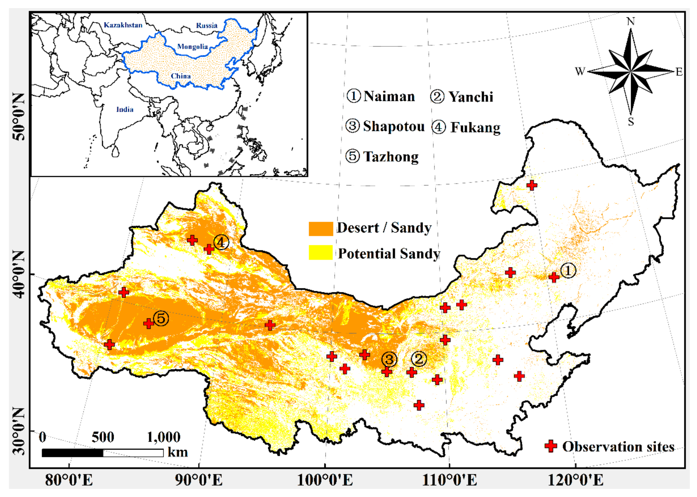
2.1. Study Area
2.2. Observed Data and Vegetation Data
2.3. Climate Projections under the Warming Scenarios
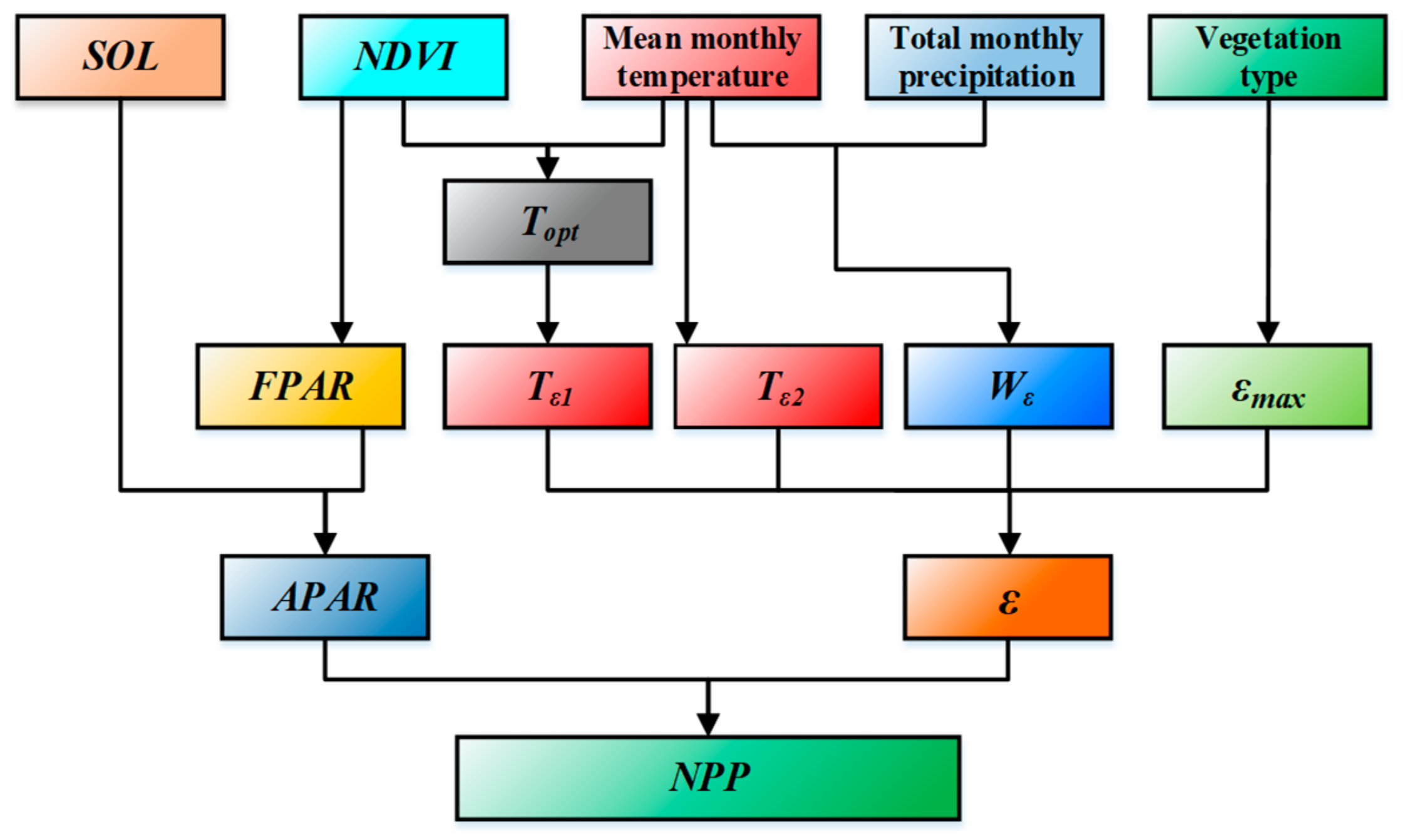
2.4. CASA Model Overview
2.5. Trend Analysis
3. Results
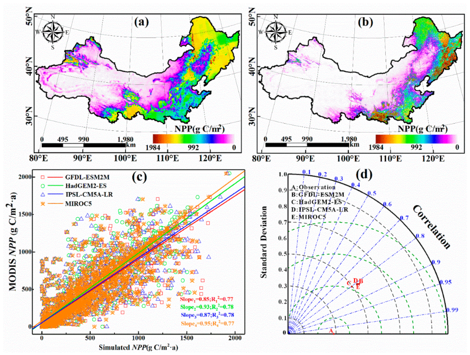
3.1. Verification of Net Primary Production Estimates
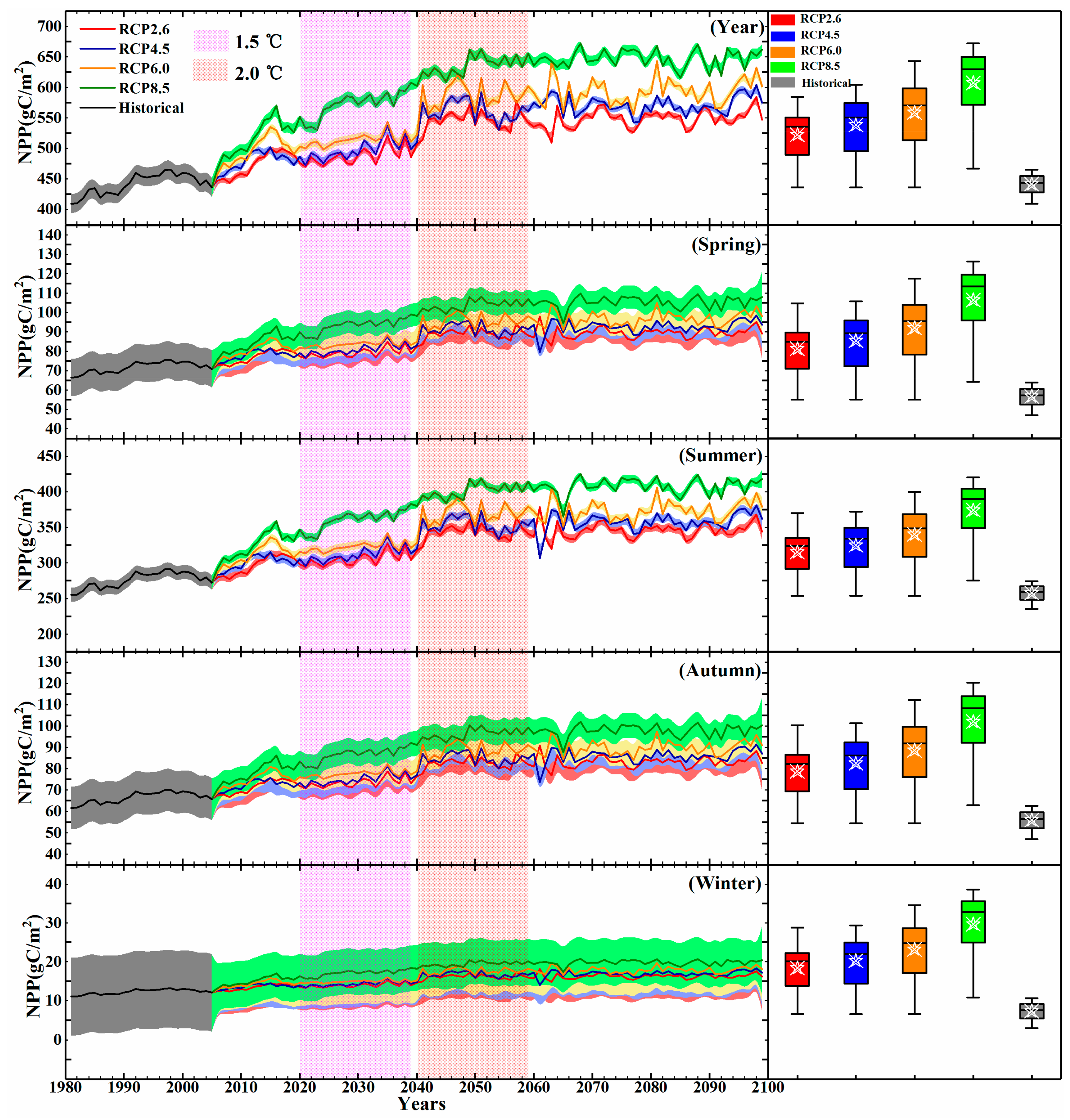
3.2. Temporal Variation in Net Primary Productivity under Different Warming Scenarios
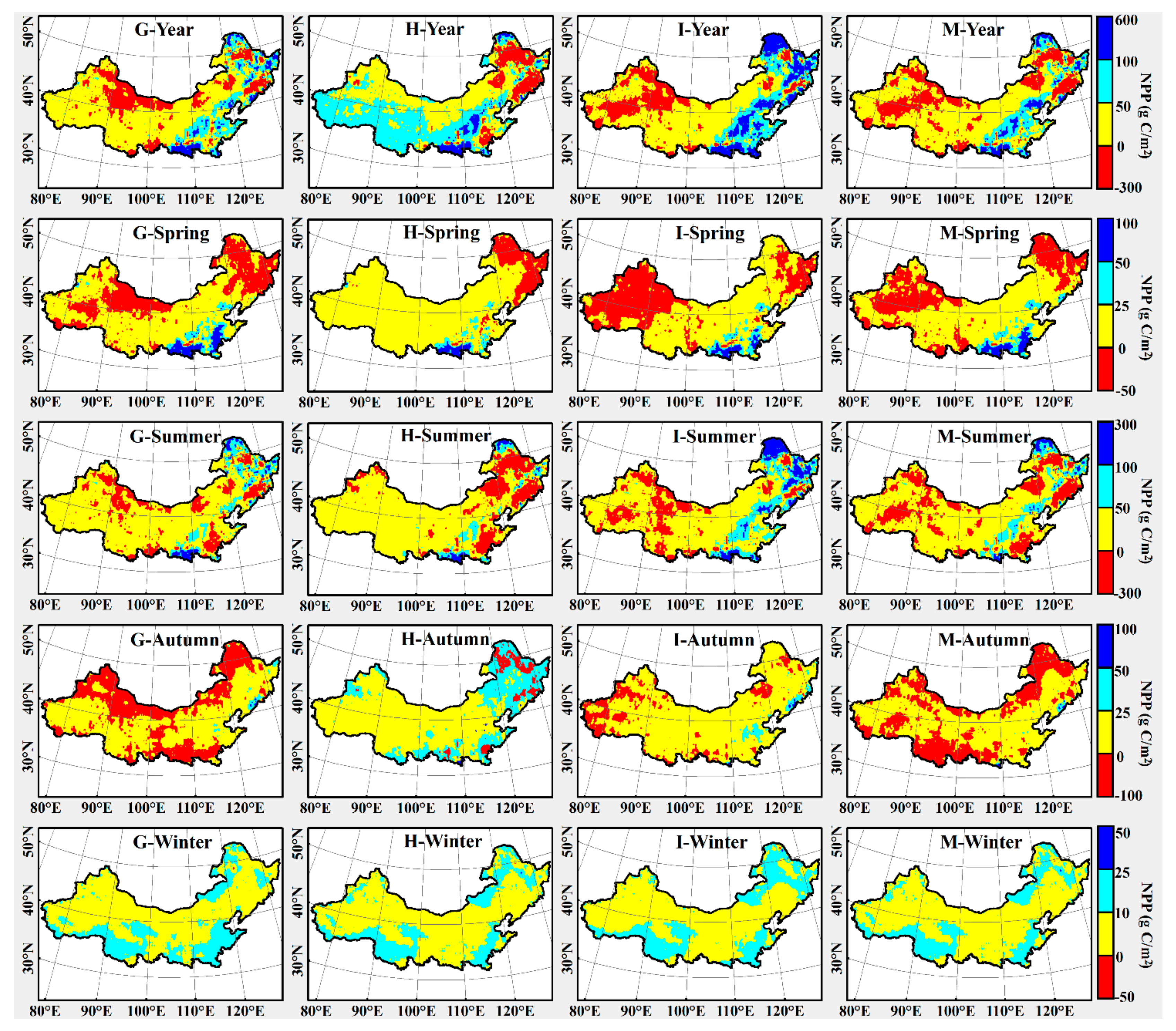
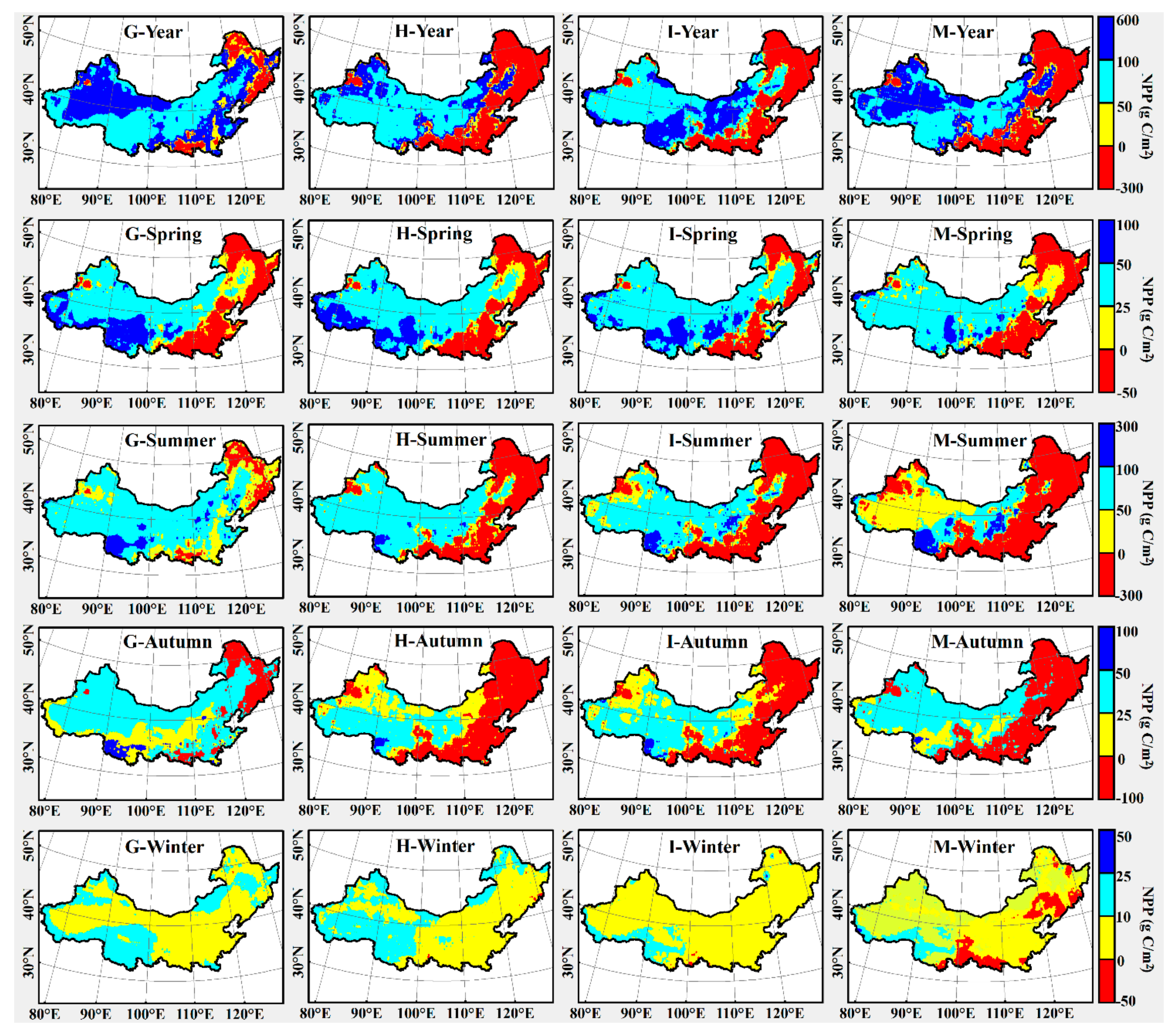
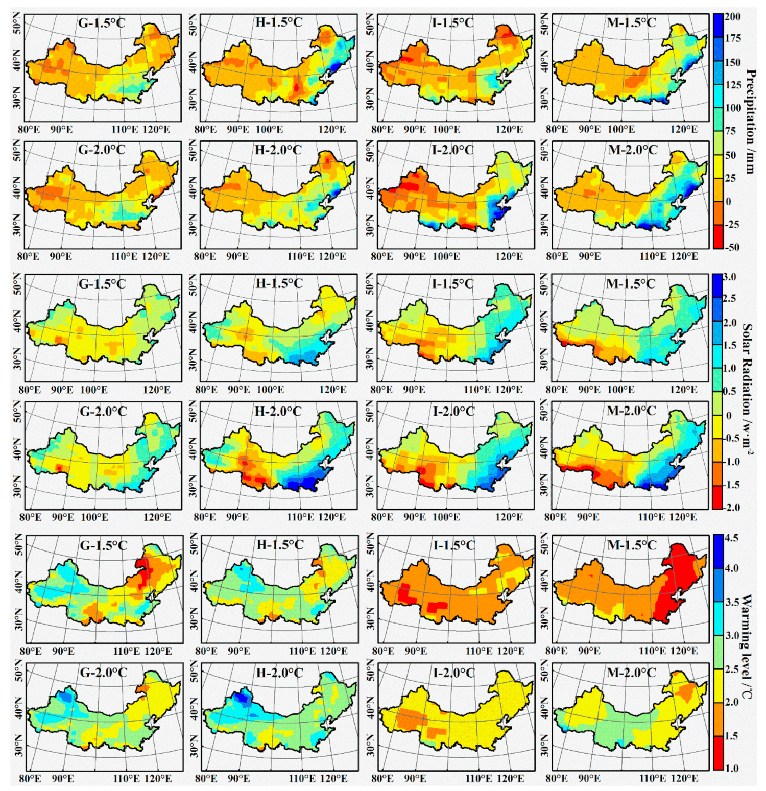
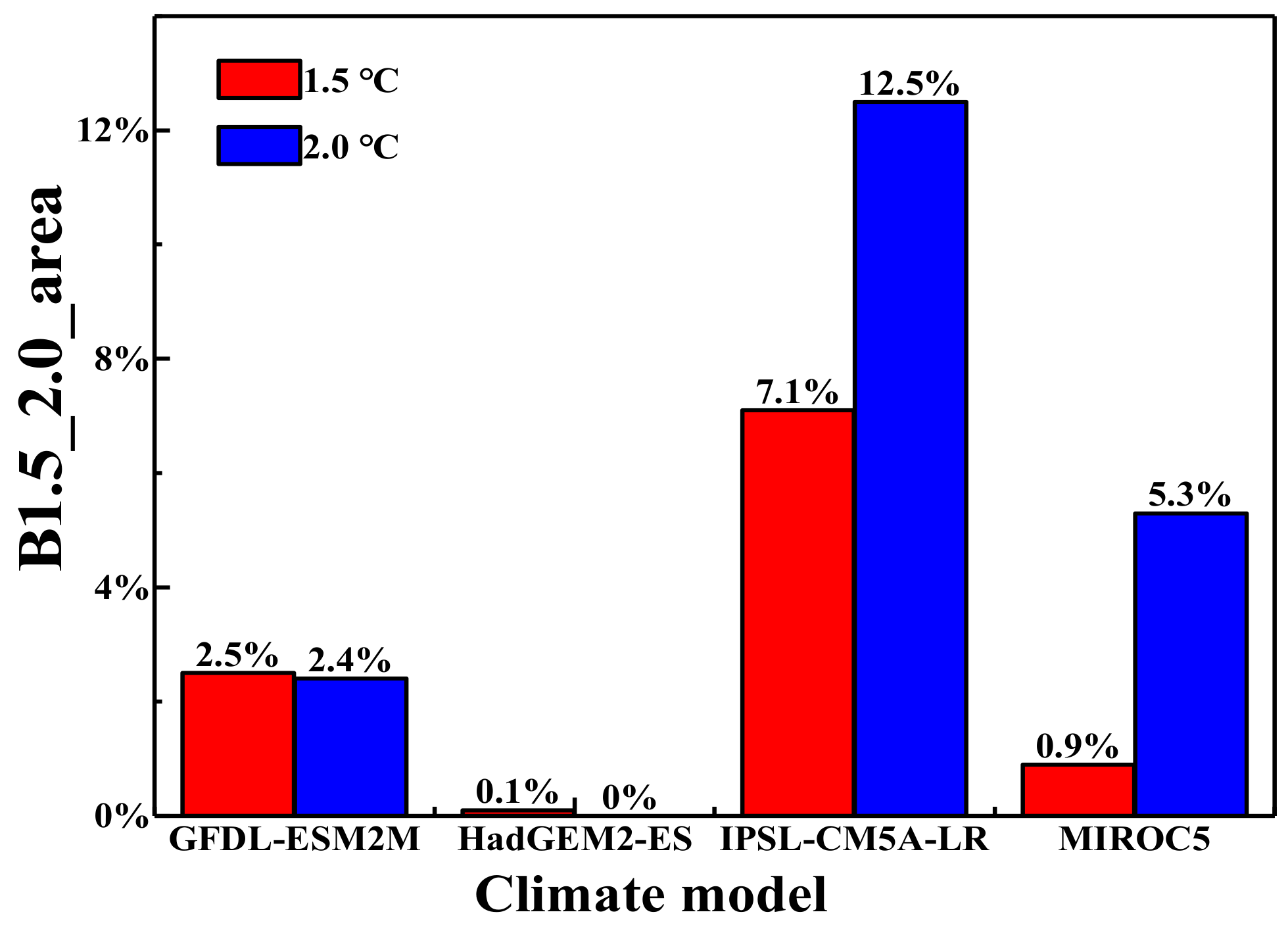
3.3. Spatial Variation in Net Primary Productivity under Warming Scenarios
4. Discussion
4.1. Impacts of Climate Variations on Net Primary Productivity in SAONC
4.2. Progress of Net Primary Productivity Simulations in SAONC
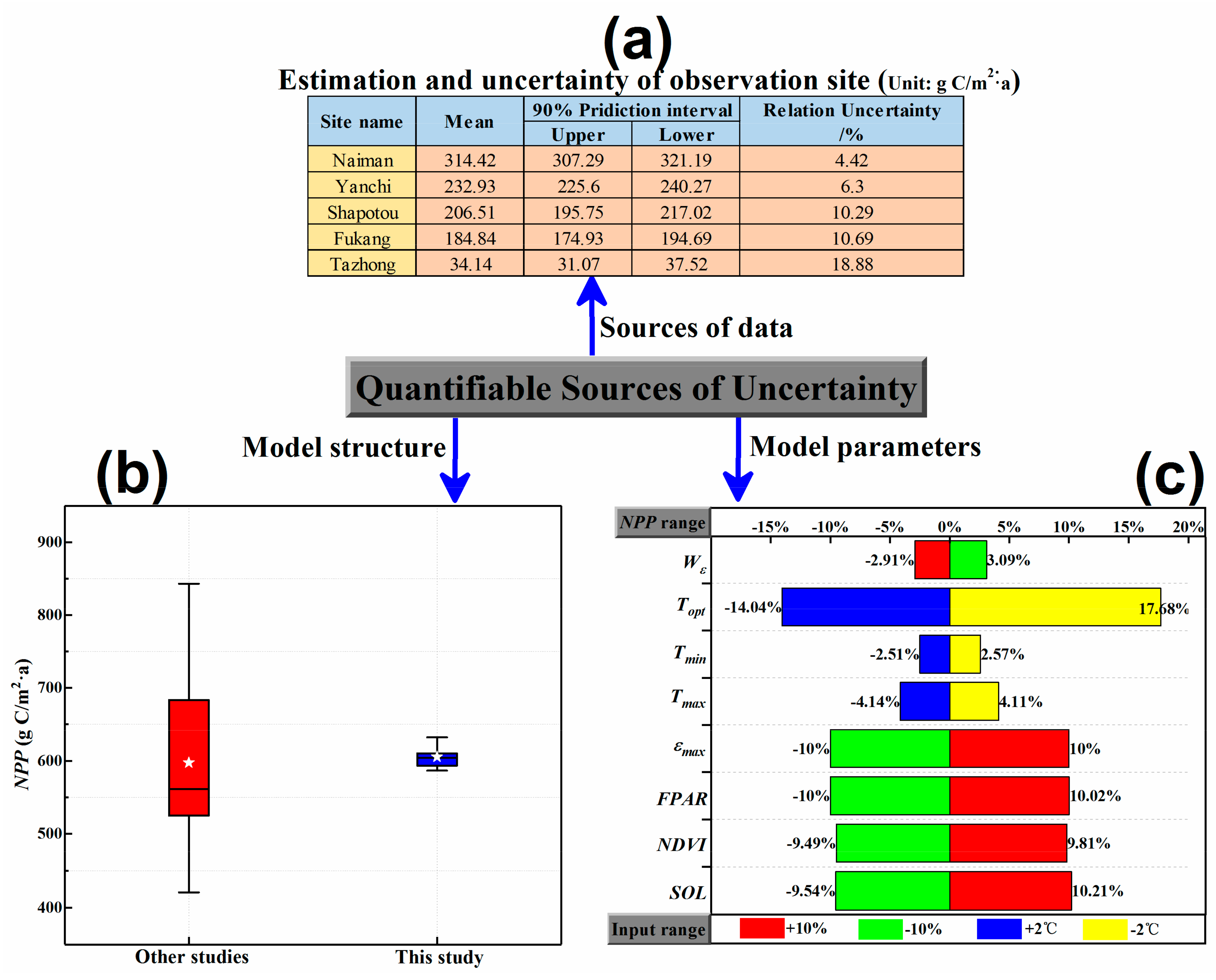
4.3. Quantifiable Sources of Uncertainty
5. Conclusions
Author Contributions
Funding
Acknowledgments
Conflicts of Interest
References
- Keeling, C.D.; Chin, J.F.S.; Whorf, T.P. Increased activity of northern vegetation inferred from atmospheric CO2 measurements. Nature 1996, 382, 146–149. [Google Scholar] [CrossRef]
- Roxburgh, S.H.; Berry, S.L.; Buckley, T.N.; Barnes, B.; Roderick, M.L. What is NPP? Inconsistent accounting of respiratory fluxes in the definition of net primary production. Funct. Ecol. 2005, 19, 378–382. [Google Scholar] [CrossRef]
- Potter, C.S.; Randerson, J.T.; Field, C.B.; Matson, P.A.; Vitousek, P.M.; Mooney, H.A.; Klooster, S.A. Terrestrial ecosystem production: A process model based on global satellite and surface data. Glob. Biogeochem. Cycle. 1993, 7, 811–841. [Google Scholar] [CrossRef]
- Cramer, W.; Kicklighter, D.W.; Bondeau, A.; Moore, B.; Churkina, G.; Nemry, B.; Ruimy, A.; Schloss, A.L.; The Participants of The Potsdam NpP Model Intercomparison. Comparing global models of terrestrial net primary productivity (NPP): Overview and key results. Glob. Change Biol. 1999, 5, 1–15. [Google Scholar] [CrossRef]
- Lehuger, S.; Gabrielle, B.; Cellier, P.; Loubet, B.; Roche, R.; Beziat, P.; Ceschia, E.; Wattenbach, M. Predicting the net carbon exchanges of crop rotations in Europe with an agro-ecosystem model. Agric. Ecosyst. Environ. 2010, 139, 384–395. [Google Scholar] [CrossRef]
- Xu, X.; Niu, S.L.; Sherry, R.A.; Zhou, X.H.; Zhou, J.Z.; Luo, Y.Q. Interannual variability in responses of belowground net primary productivity (NPP) and NPP partitioning to long-term warming and clipping in a tallgrass prairie. Glob. Change Biol. 2012, 18, 1648–1656. [Google Scholar] [CrossRef]
- Eisfelder, C.; Klein, I.; Niklaus, M.; Kuenzer, C. Net primary productivity in Kazakhstan, its spatio-temporal patterns and relation to meteorological variables. J. Arid. Environ. 2014, 103, 17–30. [Google Scholar] [CrossRef]
- Chang, J.F.; Ciais, P.; Wang, X.H.; Piao, S.L.; Asrar, G.; Betts, R.; Chevallier, F.; Dury, M.; Francois, L.; Frieler, K.; et al. Benchmarking carbon fluxes of the ISIMIP2a biome models. Environ. Res. Lett. 2017, 12, 16. [Google Scholar] [CrossRef]
- Li, Y.; Wang, Y.G.; Houghton, R.A.; Tang, L.S. Hidden carbon sink beneath desert. Geophys. Res. Lett. 2015, 42, 5880–5887. [Google Scholar] [CrossRef]
- Li, J.; Zhao, C.; Zhu, H.; Li, Y.; Wang, F. Effect of plant species on shrub fertile island at an oasis-desert ecotone in the South Junggar Basin, China. J. Arid. Environ. 2007, 71, 350–361. [Google Scholar] [CrossRef]
- Liu, Z.; Yao, Z.; Huang, H.; Wu, S.; Liu, G. Land use and climate changes and their impacts on runoff in the Yarlung Zangbo river basin, China. Land Degrad. Dev. 2014, 25, 203–215. [Google Scholar] [CrossRef]
- Stone, R. Ecosystems-Have desert researchers discovered a hidden loop in the carbon cycle? Science 2008, 320, 1409–1410. [Google Scholar] [CrossRef] [PubMed]
- Zhao, X.N.; Zhao, C.Y.; Wang, J.Y.; Stahr, K.; Kuzyakov, Y. CaCO3 recrystallization in saline and alkaline soils. Geoderma 2016, 282, 1–8. [Google Scholar] [CrossRef]
- Zhang, C.; Lu, D.S.; Chen, X.; Zhang, Y.M.; Maisupova, B.; Tao, Y. The spatiotemporal patterns of vegetation coverage and biomass of the temperate deserts in Central Asia and their relationships with climate controls. Remote Sens. Environ. 2016, 175, 271–281. [Google Scholar] [CrossRef]
- McKeon, G.M.; Stone, G.S.; Syktus, J.I.; Carter, J.O.; Flood, N.R.; Ahrens, D.G.; Bruget, D.N.; Chilcott, C.R.; Cobon, D.H.; Cowley, R.A.; et al. Climate change impacts on northern Australian rangeland livestock carrying capacity: A review of issues. Rangel. J. 2009, 31, 1–29. [Google Scholar] [CrossRef]
- Wang, P.J.; Xie, D.H.; Zhou, Y.Y.; Youhao, E.; Zhu, Q.J. Estimation of net primary productivity using a process-based model in Gansu Province, Northwest China. Environ. Earth Sci. 2014, 71, 647–658. [Google Scholar] [CrossRef]
- Li, J.; Zhao, C.Y.; Song, Y.J.; Sheng, Y.; Zhu, H. Spatial patterns of desert annuals in relation to shrub effects on soil moisture. J. Veg. Sci. 2010, 21, 221–232. [Google Scholar] [CrossRef]
- Piao, S.; Fang, J.; Ciais, P.; Peylin, P.; Huang, Y.; Sitch, S.; Wang, T. The carbon balance of terrestrial ecosystems in China. Nature 2009, 458, 1009–1013. [Google Scholar] [CrossRef]
- Lieth, H. Modeling the Primary Productivity of the World. In Primary Productivity of the Biosphere; Lieth, H., Whittaker, R.H., Eds.; Springer: Berlin/Heidelberg, Germany, 1975; pp. 237–263. [Google Scholar]
- Parton, W.J.; Scurlock, J.M.O.; Ojima, D.S.; Gilmanov, T.G.; Scholes, R.J.; Schimel, D.S.; Kirchner, T.; Menaut, J.C.; Seastedt, T.; Moya, E.G.; et al. Observations and modeling of biomass and soil organic matter dynamics for the grassland biome worldwide. Glob. Biogeochem. Cycle. 1993, 7, 785–809. [Google Scholar] [CrossRef]
- Zhu, W.Q.; Pan, Y.Z.; Liu, X.; Wang, A.L. Spatio-temporal distribution of net primary productivity along the Northeast China Transect and its response to climatic change. J. For. Res. 2006, 17, 93–98. [Google Scholar] [CrossRef]
- Zhang, M.L.; Lal, R.; Zhao, Y.Y.; Jiang, W.L.; Chen, Q.G. Estimating net primary production of natural grassland and its spatio-temporal distribution in China. Sci. Total Environ. 2016, 553, 184–195. [Google Scholar] [CrossRef] [PubMed]
- Piao, S.L.; Fang, J.Y.; Zhou, L.M.; Zhu, B.; Tan, K.; Tao, S. Changes in vegetation net primary productivity from 1982 to 1999 in China. Glob. Biogeochem. Cycle. 2005, 19, 19. [Google Scholar] [CrossRef]
- Liang, W.; Yang, Y.T.; Fan, D.M.; Guan, H.D.; Zhang, T.; Long, D.; Zhou, Y.; Bai, D. Analysis of spatial and temporal patterns of net primary production and their climate controls in China from 1982 to 2010. Agric. For. Meteorol. 2015, 204, 22–36. [Google Scholar] [CrossRef]
- Potter, C. Microclimate influences on vegetation water availability and net primary production in coastal ecosystems of Central California. Landsc. Ecol. 2014, 29, 677–687. [Google Scholar] [CrossRef]
- Nemani, R.R.; Keeling, C.D.; Hashimoto, H.; Jolly, W.M.; Piper, S.C.; Tucker, C.J.; Myneni, R.B.; Running, S.W. Climate-driven increases in global terrestrial net primary production from 1982 to 1999. Science 2003, 300, 1560–1563. [Google Scholar] [CrossRef] [PubMed]
- Piao, S.L.; Ciais, P.; Friedlingstein, P.; Peylin, P.; Reichstein, M.; Luyssaert, S.; Margolis, H.; Fang, J.Y.; Barr, A.; Chen, A.P.; et al. Net carbon dioxide losses of northern ecosystems in response to autumn warming. Nature 2008, 451, 49–52. [Google Scholar] [CrossRef]
- Field, C.B.; Randerson, J.T.; Malmstrom, C.M. Global net primary production: Combining ecology and remote sensing. Remote Sens. Environ. 1995, 51, 74–88. [Google Scholar] [CrossRef]
- Li, A.N.; Bian, J.H.; Lei, G.B.; Huang, C.Q. Estimating the Maximal Light Use Efficiency for Different Vegetation through the CASA Model Combined with Time-Series Remote Sensing Data and Ground Measurements. Remote Sens. 2012, 4, 3857–3876. [Google Scholar] [CrossRef]
- Gao, Z.Q.; Liu, J.Y. Simulation study of China’s net primary production. Chin. Sci. Bull. 2008, 53, 434–443. [Google Scholar] [CrossRef]
- Yu, D.; Shao, H.B.; Shi, P.J.; Zhu, W.Q.; Pan, Y.Z. How does the conversion of land cover to urban use affect net primary productivity? A case study in Shenzhen city, China. Agric. For. Meteorol. 2009, 149, 2054–2060. [Google Scholar]
- Stocker, T.F.; Plattner, G.K. Rethink IPCC reports. Nature 2014, 513, 163–165. [Google Scholar] [CrossRef] [PubMed][Green Version]
- Frieler, K.; Lange, S.; Piontek, F.; Reyer, C.P.O.; Schewe, J.; Warszawski, L.; Zhao, F.; Chini, L.; Denvil, S.; Emanuel, K.; et al. Assessing the impacts of 1.5 degrees C global warming-simulation protocol of the Inter-Sectoral Impact Model Intercomparison Project (ISIMIP2b). Geosci. Model Dev. 2017, 10, 4321–4345. [Google Scholar] [CrossRef]
- Schleussner, C.F.; Lissner, T.K.; Fischer, E.M.; Wohland, J.; Perrette, M.; Golly, A.; Rogelj, J.; Childers, K.; Schewe, J.; Frieler, K.; et al. Differential climate impacts for policy-relevant limits to global warming: The case of 1.5 degrees C and 2 degrees C. Earth Syst. Dynam. 2016, 7, 327–351. [Google Scholar] [CrossRef]
- Huang, J.P.; Yu, H.P.; Dai, A.G.; Wei, Y.; Kang, L.T. Drylands face potential threat under 2 degrees C global warming target. Nat. Clim. Chang. 2017, 7, 417–422. [Google Scholar] [CrossRef]
- Su, B.D.; Jian, D.N.; Li, X.C.; Wang, Y.J.; Wang, A.Q.; Wen, S.S.; Tao, H.; Hartmann, H. Projection of actual evapotranspiration using the COSMO-CLM regional climate model under global warming scenarios of 1.5 degrees C and 2.0 degrees C in the Tarim River basin, China. Atmos. Res. 2017, 196, 119–128. [Google Scholar] [CrossRef]
- Schaeffer, M.; Hare, W.; Rahmstorf, S.; Vermeer, M. Long-term sea-level rise implied by 1.5 degrees C and 2 degrees C warming levels. Nat. Clim. Chang. 2012, 2, 867–870. [Google Scholar] [CrossRef]
- Karmalkar, A.V.; Bradley, R.S. Consequences of Global Warming of 1.5 degrees C and 2 degrees C for Regional Temperature and Precipitation Changes in the Contiguous United States. PLoS ONE 2017, 12, e0168697. [Google Scholar] [CrossRef]
- Wang, X.P.; Young, M.H.; Yu, Z.; Li, X.R.; Zhang, Z.S. Long-term effects of restoration on soil hydraulic properties in revegetation-stabilized desert ecosystems. Geophys. Res. Lett. 2007, 34, 1061–1064. [Google Scholar] [CrossRef]
- Li, X.R.; Ma, F.Y.; Xiao, H.L.; Wang, X.P.; Kim, K.C. Long-term effects of revegetation on soil water content of sand dunes in arid region of Northern China. J. Arid. Environ. 2004, 57, 1–16. [Google Scholar] [CrossRef]
- Sitch, S.; Smith, B.; Prentice, I.C.; Arneth, A.; Bondeau, A.; Cramer, W.; Kaplan, J.O.; Levis, S.; Lucht, W.; Sykes, M.T.; et al. Evaluation of ecosystem dynamics, plant geography and terrestrial carbon cycling in the LPJ dynamic global vegetation model. Glob. Chang. Biol. 2003, 9, 161–185. [Google Scholar] [CrossRef]
- Ajaj, Q.M.; Pradhan, B.; Noori, A.M.; Jebur, M.N. Spatial Monitoring of Desertification Extent in Western Iraq using Landsat Images and GIS. Land Degrad. Dev. 2017, 28, 2418–2431. [Google Scholar] [CrossRef]
- Taylor, K.E.; Stouffer, R.J.; Meehl, G.A. An overview of CMIP5 and the experiment design. Bull. Amer. Meteorol. Soc. 2012, 93, 485–498. [Google Scholar] [CrossRef]
- Elguindi, N.; Grundstein, A.; Bernardes, S.; Turuncoglu, U.; Feddema, J. Assessment of CMIP5 global model simulations and climate change projections for the 21 (st) century using a modified Thornthwaite climate classification. Clim. Chang. 2014, 122, 523–538. [Google Scholar] [CrossRef]
- Chadwick, R.; Boutle, I.; Martin, G. Spatial Patterns of Precipitation Change in CMIP5: Why the Rich Do Not Get Richer in the Tropics. J. Clim. 2013, 26, 3803–3822. [Google Scholar] [CrossRef]
- Fischer, E.M.; Knutti, R. Observed heavy precipitation increase confirms theory and early models. Nat. Clim. Chang. 2016, 6, 986–991. [Google Scholar] [CrossRef]
- Miao, C.Y.; Duan, Q.Y.; Sun, Q.H.; Huang, Y.; Kong, D.X.; Yang, T.T.; Ye, A.Z.; Di, Z.H.; Gong, W. Assessment of CMIP5 climate models and projected temperature changes over Northern Eurasia. Environ. Res. Lett. 2014, 9, 055007. [Google Scholar] [CrossRef]
- Hoerling, M.P.; Eischeid, J.K.; Quan, X.W.; Diaz, H.F.; Webb, R.S.; Dole, R.M.; Easterling, D.R. Is a Transition to Semipermanent Drought Conditions Imminent in the US Great Plains? J. Clim. 2012, 25, 8380–8386. [Google Scholar] [CrossRef]
- Wuebbles, D.; Meehl, G.; Hayhoe, K.; Karl, T.R.; Kunkel, K.; Santer, B.; Wehner, M.; Colle, B.; Fischer, E.M.; Fu, R.; et al. CMIP5 climate model analyses climate extremes in the United States. Bull. Amer. Meteorol. Soc. 2014, 95, 571–583. [Google Scholar] [CrossRef]
- Marx, A.; Kumar, R.; Thober, S.; Rakovec, O.; Wanders, N.; Zink, M.; Wood, E.F.; Pan, M.; Sheffield, J.; Samaniego, L. Climate change alters low flows in Europe under global warming of 1.5, 2, and 3 degrees C. Hydrol. Earth Syst. Sci. 2018, 22, 1017–1032. [Google Scholar] [CrossRef]
- Liu, M.; Dries, L.; Heijman, W.; Huang, J.K.; Zhu, X.Q.; Hu, Y.N.; Chen, H.B. The impact of ecological construction programs on grassland conservation in Inner Mongolia, China. Land Degrad. Dev. 2018, 29, 326–336. [Google Scholar] [CrossRef]
- Yu, G.R.; Wen, X.F.; Sun, X.M.; Tanner, B.D.; Lee, X.H.; Chen, J.Y. Overview of ChinaFLUX and evaluation of its eddy covariance measurement. Agric. For. Meteorol. 2006, 137, 125–137. [Google Scholar] [CrossRef]
- Wang, K.C.; Dickinson, R.E. A review of global terrestrial evapotranspiration: Observation, modeling, climatology, and climatic variability. Rev. Geophys. 2012, 50, 54. [Google Scholar] [CrossRef]
- Aubinet, M.; Grelle, A.; Ibrom, A.; Rannik, U.; Moncrieff, J.; Foken, T.; Kowalski, A.S.; Martin, P.H.; Berbigier, P.; Bernhofer, C.; et al. Estimates of the annual net carbon and water exchange of forests: The EUROFLUX methodology. Adv. Ecol. Res. 2000, 30, 113–175. [Google Scholar]
- Webb, E.K.; Pearman, G.I.; Leuning, R. Correction of flux measurements for density effects due to heat and water-vapor transfer. Q. J. R. Meteorol. Soc. 1980, 106, 85–100. [Google Scholar] [CrossRef]
- Zomer, R.J.; Trabucco, A.; Metzger, M.J.; Wang, M.C.; Oli, K.P.; Xu, J.C. Projected climate change impacts on spatial distribution of bioclimatic zones and ecoregions within the Kailash Sacred Landscape of China, India, Nepal. Clim. Chang. 2014, 125, 445–460. [Google Scholar] [CrossRef]
- Feng, Q.; Cheng, G.D.; Endo, K.N. Water content variations and respective ecosystems of sandy land in China. Environ. Geol. 2001, 40, 1075–1083. [Google Scholar]
- Zheng, H.; Yu, G.R.; Wang, Q.F.; Zhu, X.J.; Yan, J.H.; Wang, H.M.; Shi, P.L.; Zhao, F.H.; Li, Y.N.; Zhao, L.; et al. Assessing the ability of potential evapotranspiration models in capturing dynamics of evaporative demand across various biomes and climatic regimes with ChinaFLUX measurements. J. Hydrol. 2017, 551, 70–80. [Google Scholar] [CrossRef]
- Fu, Y.L.; Yu, G.R.; Sun, X.M.; Li, Y.N.; Wen, X.F.; Zhang, L.M.; Li, Z.Q.; Zhao, L.; Hao, Y.B. Depression of net ecosystem CO2 exchange in semi-arid Leymus chinensis steppe and alpine shrub. Agric. For. Meteorol. 2006, 137, 234–244. [Google Scholar] [CrossRef]
- Yang, X.H.; He, Q.; Mamtimin, A.; Huo, W.; Liu, X.C. Diurnal variations of saltation activity at Tazhong: The hinterland of Taklimakan Desert. Meteorol. Atmos. Phys. 2013, 119, 177–185. [Google Scholar] [CrossRef][Green Version]
- Tucker, C.J.; Pinzon, J.E.; Brown, M.E.; Slayback, D.A.; Pak, E.W.; Mahoney, R.; Vermote, E.F.; El Saleous, N. An extended AVHRR 8-km NDVI dataset compatible with MODIS and SPOT vegetation NDVI data. Int. J. Remote Sens. 2005, 26, 4485–4498. [Google Scholar] [CrossRef]
- Zhang, Y.; Zhang, X.L. Estimation of net primary productivity of different forest types based on improved CASA model in Jing-Jin-Ji region, China. J. Sustain. For. 2017, 36, 568–582. [Google Scholar] [CrossRef]
- UNFCCC. UNFCCC Conference of the Parties: Adoption of the Paris Agreement; UNFCCC: Paris, France, 2015; Available online: https://unfccc.int/resource/docs/2015/cop21/eng/l09r01.pdf (accessed on 11 December 2019).
- Huang, J.P.; Ji, M.X.; Xie, Y.K.; Wang, S.S.; He, Y.L.; Ran, J.J. Global semi-arid climate change over last 60 years. Clim. Dyn. 2016, 46, 1131–1150. [Google Scholar] [CrossRef]
- Hartmann, D.L.; Tank, A.M.G.K.; Rusticucci, M.; Alexander, L.V.; Brönnimann, S.; Charabi, Y.; Dentener, F.J.; Dlugokencky, E.J.; Easterling, D.R.; Kaplan, A.; et al. Observations: Atmosphere and Surface. In Climate Change 2013: The Physical Science Basis. Contribution of Working Group I to the Fifth Assessment Report of the Intergovernmental Panel on Climate Change; Cambridge University Press: Cambridge, UK, 2013; pp. 159–254. [Google Scholar]
- Warszawski, L.; Frieler, K.; Huber, V.; Piontek, F.; Serdeczny, O.; Schewe, J. The Inter-Sectoral Impact Model Intercomparison Project (ISI-MIP): Project framework. Proc. Natl. Acad. Sci. USA 2014, 111, 3228–3232. [Google Scholar] [CrossRef] [PubMed]
- Yu, Z.; Wang, J.X.; Liu, S.R.; Rentch, J.S.; Sun, P.S.; Lu, C.Q. Global gross primary productivity and water use efficiency changes under drought stress. Environ. Res. Lett. 2017, 12, 10. [Google Scholar] [CrossRef]
- Bradford, J.B.; Hicke, J.A.; Lauenroth, W.K. The relative importance of light-use efficiency modifications from environmental conditions and cultivation for estimation of large-scale net primary productivity. Remote Sens. Environ. 2005, 96, 246–255. [Google Scholar] [CrossRef]
- Mahamah, D.S. Simplified sensitivity analysis applied to a nutrient-biomass model. Ecol. Model. 1988, 42, 103–109. [Google Scholar] [CrossRef]
- Yan, Y.A.; Wang, S.Q.; Wang, Y.D.; Wu, W.X.; Wang, J.Y.; Chen, B.; Yang, F.T. Assessing productivity and carbon sequestration capacity of subtropical coniferous plantations using the process model PnET-CN. J. Geogr. Sci. 2011, 21, 458–474. [Google Scholar] [CrossRef]
- Li, S.S.; Lu, S.H.; Zhang, Y.J.; Liu, Y.P.; Gao, Y.H.; Ao, Y.H. The change of global terrestrial ecosystem net primary productivity (NPP) and its response to climate change in CMIP5. Theor. Appl. Climatol. 2015, 121, 319–335. [Google Scholar] [CrossRef]
- Li, S.S.; Lu, S.H.; Liu, Y.P.; Gao, Y.H.; Ao, Y.H. Variations and trends of terrestrial NPP and its relation to climate change in the 10 CMIP5 models. J. Earth Syst. Sci. 2015, 124, 395–403. [Google Scholar] [CrossRef]
- Xu, X.; Sherry, R.A.; Niu, S.L.; Li, D.J.; Luo, Y.Q. Net primary productivity and rain-use efficiency as affected by warming, altered precipitation, and clipping in a mixed-grass prairie. Glob. Change Biol. 2013, 19, 2753–2764. [Google Scholar] [CrossRef]
- Beer, C.; Reichstein, M.; Tomelleri, E.; Ciais, P.; Jung, M.; Carvalhais, N.; Rodenbeck, C.; Arain, M.A.; Baldocchi, D.; Bonan, G.B.; et al. Terrestrial Gross Carbon Dioxide Uptake: Global Distribution and Covariation with Climate. Science 2010, 329, 834–838. [Google Scholar] [CrossRef] [PubMed]
- Zhao, C.Y.; Wang, Y.C.; Hu, S.J.; Li, Y. Effects of spatial variability on estimation of evapotranspiration in the continental river basin. J. Arid. Environ. 2004, 56, 373–382. [Google Scholar] [CrossRef]
- Fang, J.Y.; Piao, S.L.; Field, C.B.; Pan, Y.D.; Guo, Q.H.; Zhou, L.M.; Peng, C.H.; Tao, S. Increasing net primary production in China from 1982 to 1999. Front. Ecol. Environ. 2003, 1, 293–297. [Google Scholar] [CrossRef]
- Li, F.; Zhao, W.Z.; Liu, H. Productivity responses of desert vegetation to precipitation patterns across a rainfall gradient. J. Plant Res. 2015, 128, 283–294. [Google Scholar] [CrossRef]
- Zhao, C.Y.; Wang, Y.C.; Chen, X.; Li, B.G. Simulation of the effects of groundwater level on vegetation change by combining FEFLOW software. Ecol. Model. 2005, 187, 341–351. [Google Scholar] [CrossRef]
- Gang, C.C.; Wang, Z.Q.; Zhou, W.; Chen, Y.Z.; Li, J.L.; Cheng, J.M.; Guo, L.; Odeh, I.; Chen, C. Projecting the dynamics of terrestrial net primary productivity in response to future climate change under the RCP2.6 scenario. Environ. Earth Sci. 2015, 74, 5949–5959. [Google Scholar] [CrossRef]
- Sun, G.D.; Mu, M. Understanding variations and seasonal characteristics of net primary production under two types of climate change scenarios in China using the LPJ model. Clim. Chang. 2013, 120, 755–769. [Google Scholar] [CrossRef]
- Li, Z.; Pan, J.H. Spatiotemporal changes in vegetation net primary productivity in the arid region of Northwest China, 2001 to 2012. Front. Earth Sci. 2018, 12, 108–124. [Google Scholar] [CrossRef]
- Piao, S.; Fang, J. Terrestrial net primary production and its spatio-temporal patterns in Qinghai-Xizang Plateau, China during 1982-1999. J. Nat. Resour. 2002, 17, 373–380. [Google Scholar]
- Chen, L.; Liu, G.; Li, H. Estimating Net Primary Productivity of Terrestrial Vegetation in China Using Remote Sensing. J. Remote Sens. 2002, 6, 129–135. [Google Scholar]
- Cao, M.K.; Tao, B.; Li, K.R.; Shao, X.M.; Prience, S.D. Interannual variation in terrestrial ecosystem carbon fluxes in China from 1981 to 1998. Acta Bot. Sin. 2003, 45, 552–560. [Google Scholar]
- Feng, X.; Liu, G.; Chen, J.M.; Chen, M.; Liu, J.; Ju, W.M.; Sun, R.; Zhou, W. Net primary productivity of China’s terrestrial ecosystems from a process model driven by remote sensing. J. Environ. Manag. 2007, 85, 563–573. [Google Scholar] [CrossRef] [PubMed]
- Chen, B.; Shaoqiang, W.; Ronggao, L.; Ting, S. Study on Modeling and Spatial Pattern of Net Primary Production in China’s Terrestrial Ecosystem. Resour. Sci. 2007, 29, 45–53. [Google Scholar]
- Zhao, D.S.; Wu, S.H. Vulnerability of natural ecosystem in China under regional climate scenarios: An analysis based on eco-geographical regions. J. Geogr. Sci. 2014, 24, 237–248. [Google Scholar] [CrossRef]
- Mao, J.F.; Dan, L.; Wang, B.; Dai, Y.J. Simulation and evaluation of terrestrial ecosystem NPP with M-SDGVM over continental China. Adv. Atmos. Sci. 2010, 27, 427–442. [Google Scholar] [CrossRef]
- Chen, F.; Shen, Y.; Li, Q.; Guo, Y.; Xu, L. Spatio-temporal Variation Analysis of Ecological Systems NPP in China in Past 30 years. Sci. Geogr. Sin. 2011, 31, 1409–1414. [Google Scholar]
- Liu, Y.B.; Ju, W.M.; He, H.L.; Wang, S.Q.; Sun, R.; Zhang, Y.D. Changes of net primary productivity in China during recent 11 years detected using an ecological model driven by MODIS data. Front. Earth Sci. 2013, 7, 112–127. [Google Scholar] [CrossRef]
- Pei, F.S.; Li, X.; Liu, X.P.; Lao, C.H. Assessing the impacts of droughts on net primary productivity in China. J. Environ. Manag. 2013, 114, 362–371. [Google Scholar] [CrossRef]
- Ji, J.J.; Huang, M.; Li, K.R. Prediction of carbon exchanges between China terrestrial ecosystem and atmosphere in 21st century. Sci. China Ser. D-Earth Sci. 2008, 51, 885–898. [Google Scholar] [CrossRef]
- Wu, S.H.; Yin, Y.H.; Zhao, D.S.; Huang, M.; Shao, X.M.; Dai, E.F. Impact of future climate change on terrestrial ecosystems in China. Int. J. Climatol. 2010, 30, 866–873. [Google Scholar] [CrossRef]
- Ju, W.M.; Chen, J.M.; Harvey, D.; Wang, S. Future carbon balance of China’s forests under climate change and increasing CO2. J. Environ. Manag. 2007, 85, 538–562. [Google Scholar] [CrossRef]
- Wen, Z.; Yao, H.; Wenjuan, S.J.; Yongqiang, Y.Q. Simulating crop net primary production in China from 2000 to 2050 by linking the crop-C model with a FGOALS’s model climate change scenario. Adv. Atmos. Sci. 2007, 24, 845–854. [Google Scholar]
- Tao, F.L.; Zhang, Z. Dynamic responses of terrestrial ecosystems structure and function to climate change in China. J. Geophys. Res.-Biogeosci. 2010, 115, 58–72. [Google Scholar] [CrossRef]
- Pretis, F.; Schwarz, M.; Tang, K.; Haustein, K.; Allen, M.R. Uncertain impacts on economic growth when stabilizing global temperatures at 1.5°C or 2°C warming. Philos. Trans. R. Soc. A Math. Phys. Eng. Sci. 2018, 376, 20160460. [Google Scholar] [CrossRef] [PubMed]
- Ito, A. Decadal Variability in the Terrestrial Carbon Budget Caused by the Pacific Decadal Oscillation and Atlantic Multidecadal Oscillation. J. Meteorol. Soc. Jpn. 2011, 89, 441–454. [Google Scholar] [CrossRef]
- Shafran Nathan, R.; Svoray, T.; Perevolotsky, A. The resilience of annual vegetation primary production subjected to different climate change scenarios. Clim. Chang. 2013, 118, 227–243. [Google Scholar] [CrossRef]
- Shao, P.; Zeng, X.B.; Sakaguchi, K.; Monson, R.K.; Zeng, X.D. Terrestrial Carbon Cycle: Climate Relations in Eight CMIP5 Earth System Models. J. Clim. 2013, 26, 8744–8764. [Google Scholar] [CrossRef]
- Finstad, A.G.; Hein, C.L. Migrate or stay: Terrestrial primary productivity and climate drive anadromy in Arctic char. Glob. Change Biol. 2012, 18, 2487–2497. [Google Scholar] [CrossRef]
- Gurney, K.R.; Law, R.M.; Denning, A.S.; Rayner, P.J.; Baker, D.; Bousquet, P.; Bruhwiler, L.; Chen, Y.H.; Ciais, P.; Fan, S.M.; et al. TransCom 3 CO2 inversion intercomparison: 1. Annual mean control results and sensitivity to transport and prior flux information. Tellus Ser. B-Chem. Phys. Meteorol. 2003, 55, 555–579. [Google Scholar] [CrossRef]
- Bondeau, A.; Kicklighter, D.W.; Kaduk, J.; The Participants of The Potsdam NpP Model Intercomparison. Comparing global models of terrestrial net primary productivity (NPP): Importance of vegetation structure on seasonal NPP estimates. Glob. Change Biol. 1999, 5, 35–45. [Google Scholar] [CrossRef]
- Adams, B.; White, A.; Lenton, T.M. An analysis of some diverse approaches to modelling terrestrial net primary productivity. Ecol. Model. 2004, 177, 353–391. [Google Scholar] [CrossRef]
- Baldocchi, D. Breathing of the terrestrial biosphere: Lessons learned from a global network of carbon dioxide flux measurement systems. Aust. J. Bot. 2008, 56, 1–26. [Google Scholar] [CrossRef]
- Patra, P.K.; Ishizawa, M.; Maksyutov, S.; Nakazawa, T.; Inoue, G. Role of biomass burning and climate anomalies for land-atmosphere carbon fluxes based on inverse modeling of atmospheric CO2. Glob. Biogeochem. Cycle. 2005, 19, 15. [Google Scholar] [CrossRef]
- Sarmiento, J.L.; Lequere, C.; Pacala, S.W. Limiting future atmospheric carbon dioxide. Glob. Biogeochem. Cycle. 1995, 9, 121–137. [Google Scholar] [CrossRef]
- Zhu, Q.; Zhuang, Q.L. Parameterization and sensitivity analysis of a process-based terrestrial ecosystem model using adjoint method. J. Adv. Model. Earth Syst. 2014, 6, 315–331. [Google Scholar] [CrossRef]
- Huang, N.; Niu, Z.; Wu, C.Y.; Tappert, M.C. Modeling net primary production of a fast-growing forest using a light use efficiency model. Ecol. Model. 2010, 221, 2938–2948. [Google Scholar] [CrossRef]
- Doughty, C.E.; Metcalfe, D.B.; Girardin, C.A.J.; Amezquita, F.F.; Cabrera, D.G.; Huasco, W.H.; Silva-Espejo, J.E.; Araujo-Murakami, A.; da Costa, M.C.; Rocha, W.; et al. Drought impact on forest carbon dynamics and fluxes in Amazonia. Nature 2015, 519, 78–82. [Google Scholar] [CrossRef]
- Fu, W.W.; Randerson, J.T.; Moore, J.K. Climate change impacts on net primary production (NPP) and export production (EP) regulated by increasing stratification and phytoplankton community structure in the CMIP5 models. Biogeosciences 2016, 13, 5151–5170. [Google Scholar] [CrossRef]
- Zheng, D.L.; Prince, S.; Wright, R. Terrestrial net primary production estimates for 0.5 degrees grid cells from field observations-a contribution to global biogeochemical modeling. Glob. Chang. Biol. 2003, 9, 46–64. [Google Scholar] [CrossRef]
- Zhao, M.S.; Heinsch, F.A.; Nemani, R.R.; Running, S.W. Improvements of the MODIS terrestrial gross and net primary production global data set. Remote Sens. Environ. 2005, 95, 164–176. [Google Scholar] [CrossRef]


| Site Name | Lat (° N) | Lon (° E) | Precipitation (mm) | Height (m) | Bioclimate Region | Reference |
|---|---|---|---|---|---|---|
| Naiman | 42.93 | 120.7 | 366.4 | 361 | Semi-humid | Zheng et al. [58] |
| Yanchi | 37.4 | 107.12 | 295 | 442 | Semi-arid | Fu et al. [59] |
| Shapotou | 37.53 | 105.8 | 186.6 | 1227 | Arid | Zheng et al. [58] |
| Fukang | 42.28 | 87.92 | 160 | 482 | Arid | Yu et al. [52] |
| Tazhong | 38.97 | 83.65 | 22.8 | 1082 | Extremely arid | Yang et al. [60] |
| Model | Institution | Country | Resolution (Lon × Lat) |
|---|---|---|---|
| GFDL-ESM2M | Geophysical Fluid Dynamics Laboratory | USA | 144 × 90 |
| HadGEM2-ES | Met Office Hadley Center | UK | 145 × 192 |
| IPSL-CM5A-LR | L’ Institute Pierre-Simon Laplace | France | 96 × 96 |
| MIROC5 | Model for Interdisciplinary Research on Climate | Japan | 256 × 128 |
| Emission Scenarios | ISI-MIP 2b | Precipitation | Temperature | Solar Radiation |
|---|---|---|---|---|
| RCP2.6 | GFDL-ESM2M | 0.198 * | 0.672 ** | 0.481 ** |
| HadGEM2-ES | 0.505 ** | 0.812 ** | 0.493 ** | |
| IPSL-CM5A-LR | 0.494 ** | 0.787 ** | 0.425 ** | |
| MIROC5 | 0.555 ** | 0.847 ** | 0.647 ** | |
| RCP4.5 | GFDL-ESM2M | 0.355 ** | 0.853 ** | 0.215 * |
| HadGEM2-ES | 0.500 ** | 0.882 ** | 0.356 ** | |
| IPSL-CM5A-LR | 0.453 ** | 0.883 ** | 0.512 ** | |
| MIROC5 | 0.537 ** | 0.88 3** | 0.352 ** | |
| RCP6.0 | GFDL-ESM2M | 0.017 | 0.642 ** | −0.239 |
| HadGEM2-ES | 0.202 | 0.702 ** | −0.192 | |
| IPSL-CM5A-LR | 0.072 | 0.742 ** | −0.325 * | |
| MIROC5 | 0.017 | 0.614 ** | −0.490 ** | |
| RCP8.5 | GFDL-ESM2M | 0.390 ** | 0.863 ** | 0.062 |
| HadGEM2-ES | 0.674 ** | 0.850 ** | −0.223 * | |
| IPSL-CM5A-LR | 0.598 ** | 0.850 ** | 0.213 * | |
| MIROC5 | 0.752 ** | 0.870 ** | −0.087 |
| Methods | Study Periods | NPP Ranges (g C/m2) | Reference |
|---|---|---|---|
| LPJ model | 1961–1970 | 686.75 | Sun and Mu [80] |
| CASA model | 2000–2012 | 556.29 | Li and Pan [81] |
| CASA model | 1982–1999 | 510.72 | Piao and Fang [82] |
| LUE model | 1990 | 584.75 | Chen et al. [83] |
| CEVSE model | 1981–1998 | 420.49 | Cao et al. [84] |
| CASA model | 1982–1999 | 523.59 | Fang et al. [76] |
| BEPS model | 2001 | 558.29 | Feng et al. [85] |
| C-Fix model | 2003 | 654.17 | Chen et al. [86] |
| CASA model | 1989–1993 | 483.19 | Zhu et al. [21] |
| GLO-PEM model | 1981–2000 | 710.49 | Gao and Liu [30] |
| CEVSA model | 1980–2000 | 667.45 | Gao and Liu [30] |
| GEOPRO model | 2000 | 683.29 | Gao and Liu [30] |
| GEO-LUE model | 2000–2004 | 724.54 | Gao and Liu [30] |
| LPJ model | 1961–2080 | 564.42 | Zhao and Wu [87] |
| M-SDGVM | 1981–2000 | 537.24 | Mao et al. [88] |
| CASA model | 1981–2008 | 487.69 | Chen et al. [89] |
| BEPS model | 2000–2010 | 684.29 | Liu et al. [90] |
| CASA model | 2000–2010 | 526.47 | Pei et al. [91] |
| CASA model | 1982–2010 | 545.29 | Liang et al. [24] |
| CSCS model | 2030 2050 2070 | 843.27 | Gang et al. [79] |
| CASA model | 1980–2100 | 604.52 | This study |
© 2020 by the authors. Licensee MDPI, Basel, Switzerland. This article is an open access article distributed under the terms and conditions of the Creative Commons Attribution (CC BY) license (http://creativecommons.org/licenses/by/4.0/).
Share and Cite
Ma, X.; Huo, T.; Zhao, C.; Yan, W.; Zhang, X. Projection of Net Primary Productivity under Global Warming Scenarios of 1.5 °C and 2.0 °C in Northern China Sandy Areas. Atmosphere 2020, 11, 71. https://doi.org/10.3390/atmos11010071
Ma X, Huo T, Zhao C, Yan W, Zhang X. Projection of Net Primary Productivity under Global Warming Scenarios of 1.5 °C and 2.0 °C in Northern China Sandy Areas. Atmosphere. 2020; 11(1):71. https://doi.org/10.3390/atmos11010071
Chicago/Turabian StyleMa, Xiaofei, Tianci Huo, Chengyi Zhao, Wei Yan, and Xun Zhang. 2020. "Projection of Net Primary Productivity under Global Warming Scenarios of 1.5 °C and 2.0 °C in Northern China Sandy Areas" Atmosphere 11, no. 1: 71. https://doi.org/10.3390/atmos11010071
APA StyleMa, X., Huo, T., Zhao, C., Yan, W., & Zhang, X. (2020). Projection of Net Primary Productivity under Global Warming Scenarios of 1.5 °C and 2.0 °C in Northern China Sandy Areas. Atmosphere, 11(1), 71. https://doi.org/10.3390/atmos11010071