Development of a Building-Scale Meteorological Prediction System Including a Realistic Surface Heating

Abstract

Microscale urban meteorological models have been widely used in interpreting atmospheric flow and thermal discomfort in urban environments, but most previous studies examined the urban flow and thermal environments for an idealized urban morphology with imposing neutral or homogeneous thermal forcing. This study has developed a new building-scale meteorological prediction system that extends the ability to predict microscale meteorological fields in real urban environments. A computational fluid dynamics (CFD) model has been developed based on the non-hydrostatic incompressible Reynolds-averaged Navier-Stokes (RANS) equations with a standard k-ε turbulence model, and the microscale urban surface energy (MUSE) model was coupled with the CFD model to provide realistic surface thermal boundary conditions in real urban environments. It is driven by the large scale wind and temperature fields predicted by the Korean operational weather prediction model. The validation results of the new building-scale meteorological prediction system were presented against wind tunnel data and field measurements, showing its ability to predict in-canyon flows and thermal environments in association with spatiotemporal variations of surface temperatures in real urban environments. The effects of realistic surface heating on pedestrian level wind and thermal environments have been investigated through sensitivity simulations of different surface heating conditions in the highly built-up urban area. The results implied that the inclusion of surface thermal forcing is important in interpreting urban flow and thermal environment of the urban area, highlighting a realistic urban surface heating that should be considered in predicting building-scale meteorology over real urban environments.

1. Introduction

Rapid urbanization, which is projected that two-thirds of the world’s population would live in cities by 2050 [1], causes various environmental problems in association with unique micrometeorological states in urban areas (e.g., [2,3]). Urban surfaces are mostly characterized by buildings, roads, and permeable natural surfaces, and various physical processes such as radiative trapping, turbulence heat exchange, sub-surface thermal conduction occur, which results in unique urban micrometeorology. Thus, understanding of the local micrometeorology is important to minimize various environmental problems that have occurred in urban areas. Many wind tunnel experiments and field measurements have been conducted to understand the urban meteorological environments (e.g., [4,5,6,7,8]). Wind tunnel experiments have advantages in collecting high-density spatial data and in interpreting microscale flow and thermal structures because wind tunnel data are obtained from well-designed experimental setups in terms of ideal/real cities’ morphological structures and meteorological driving forcing (e.g., [4,6]). However, they have limitations in that the multiscale meteorological influences in the urban boundary layer (UBL) are not considered. Field measurements can collect the meteorological data that reflect the UBL influences in the real urban area of interest, which compensates the wind tunnel experiments to some extent. However, the spatial density of the measurement data is generally not enough to resolve the microscale meteorological states of an urban area (e.g., [7,8]).

Microscale meteorological models have been widely used in investigating atmospheric flow, dispersion, and thermal comfort conditions in urban environments, compensating for the limitations in the wind tunnel experiments and field measurements (e.g., [9,10,11,12,13,14,15,16,17]). Kim and Baik [9] found that urban morphology is an important factor in determining in-canyon flow and turbulence in an ideal two-dimensional canyon morphology using a computational fluid dynamics (CFD) model. Park et al. [12] examined the effects of homogeneous wall surface heating on in-canyon flow applying a large-eddy simulation (LES) model for a single canyon circulation simulation, which showed the wall surface heating can alter the in-canyon vortex circulation in shape and strength. Recently, microscale meteorological applications to real urban environments are increasing by virtue of the increase of available computer resources and the enhancement of the geographic information system (GIS) data (e.g., [18,19,20]). Gronemeier et al. [18] and Wang et al. [20] examined air ventilation under unstable atmospheric boundary layer in the highly built-up urban area of Hong Kong by imposing a homogeneous surface heating within the parallelized large-eddy simulation model (PALM). The studies reported that homogeneous surface heating led to an increase in pedestrian-level velocity ratio and wind directional change. Meanwhile, Nazarian and Kleissl [15] investigated the effects of in-canyon heterogeneous surface heating on atmospheric flow over an idealized cube array configuration, for which an urban surface energy balance model [21] was used to predict spatial and temporal variations of the surface temperatures. The results showed that heterogeneous surface heating modified the mean atmospheric flows and turbulent transfer efficiency particularly under strong unstable atmospheric conditions.

The previous studies have examined characteristic features of urban flow and thermal environments for an idealized urban morphology with imposing heterogeneous surface heating or for a real urban area with imposing neutral or homogeneous thermal forcing. This study aims to develop a new building-scale meteorological prediction system in order to extend the ability to predict microscale meteorological fields with realistic surface heating in real urban environments. In doing so, heterogeneous surface temperatures of the urban facets of a highly built-up real urban area have been considered using the microscale urban surface energy (MUSE) model. It also investigates the effects of heterogeneous thermal forcing on pedestrian-level wind and thermal environments in the highly built-up urban area. The remainder of the manuscript is structured as follows: Section 2 describes the newly developed building-scale meteorological prediction system and Section 3 presents validation results of the building-scale meteorological prediction system against wind tunnel data and field measurements. Section 4 discusses the effects of realistic surface heating on pedestrian-level wind and thermal environments in the highly built-up urban area, and summary and conclusions are followed in Section 5.

2. Description of the Building-Scale Meteorological Prediction System

2.1. Computational Fluid Dynamics (CFD) Model

2.2.1. The Governing Equations

The CFD model has been developed based on the dynamic equations and numerical methods in Baik et al. [10]. The governing equations consist of the Reynolds-averaged conservation equations of mass, momentum, and heat under the Boussinesq approximation as follows [10,22,23]:

$$\frac{\partial {\overline{u}}_j}{\partial x_j}=0,$$

(1)

$$\frac{\partial {\overline{u}}_i}{\partial t}=-{\overline{u}}_j\frac{\partial {\overline{u}}_i}{\partial x_j}-\frac{1}{{\rho }_0}\frac{\partial P^{*}}{\partial x_i}+g\frac{T-T_0}{T_0}{\delta }_{i3}+\nu \frac{{\partial }^2{\overline{u}}_i}{\partial x_j\partial x_j}-\frac{\partial \overline{u_i^{\prime }{u}_j^{\prime }}}{\partial x_j},$$

(2)

$$\frac{\partial \overline{T}}{\partial t}=-{\overline{u}}_j\frac{\partial \overline{T}}{\partial x_j}+\kappa \frac{{\partial }^2\overline{T}}{\partial x_j\partial x_j}-\frac{\partial \overline{T^{\prime }{u}_j^{\prime }}}{\partial x_j}+Q_T.$$

(3)

Here, ${\overline{u}}_i$ is the Reynolds-averaged wind velocity component in the ith space coordinate of $x_i$, $\rho$ is the air density, $P^{*}$ is the pressure perturbation from the reference state, $T$ is the Reynolds-averaged air temperature; $u_i^{\prime }$ and $T^{\prime }$ are the perturbation fields of ith wind velocity component and temperature, respectively; ${\rho }_0$ and are $T_0$ are the air density and temperature of the reference state, respectively; ν and κ are the kinematic viscosity and molecular thermal diffusivity of the air, respectively; ${\delta }_{i3}$ is the Kronecker delta and $g$ is the gravitational acceleration; $Q_T$ is the diabatic source term; $t$ is the time. $\overline{u_i^{\prime }{u}_j^{\prime }}$ and $\overline{T^{\prime }{u}_j^{\prime }}$ represent the Reynolds stresses and turbulent heat fluxes, respectively, which are parameterized using the K-theory as follows [24]:

$$\overline{u_i^{\prime }{u}_j^{\prime }}=-K_m\left(\frac{\partial {\overline{u}}_i}{\partial x_j}+\frac{\partial {\overline{u}}_j}{\partial x_i}\right)+\frac{2}{3}{\delta }_{ij}k,$$

(4)

$$\overline{T^{\prime }{u}_j^{\prime }}=K_T\frac{\partial \overline{T}}{\partial x_j},$$

(5)

where $K_m$ and $K_h$ are the eddy diffusivity of momentum and heat, respectively, and $k$ is the turbulent kinetic energy. The eddy diffusivity of momentum is expressed as a function of the turbulent kinetic energy ($k$) and its dissipation rate ($\epsilon$) as follows:

$$K_m=C_{\mu }\frac{k^2}{\epsilon },$$

(6)

where $C_{\mu }$ is the empirical constant (=0.09). The eddy diffusivity of heat can be expressed by the turbulent Prandtl number ($Pr$) (=0.7) as follows:

$$K_T=\frac{K_m}{Pr}.$$

(7)

The turbulent kinetic energy ($k$) and its dissipation rate ($\epsilon$) are solved from the prognostic turbulence equations:

$$\frac{\partial k}{\partial t}=-{\overline{u}}_j\frac{\partial k}{\partial x_j}-\overline{u_i^{\prime }{u}_j^{\prime }}\frac{\partial \overline{u_i}}{\partial x_j}+\frac{{\delta }_{3j}g}{T_0}\overline{T^{\prime }{u}_j^{\prime }}+\frac{\partial }{\partial x_i}\left(\frac{K_m}{{\sigma }_k}\frac{\partial k}{\partial x_j}\right)-\epsilon ,$$

(8)

$$\frac{\partial \epsilon }{\partial t}=-{\overline{u}}_j\frac{\partial \epsilon }{\partial x_j}-C_{\epsilon 1}\frac{\epsilon }{k}\overline{u_i^{\prime }{u}_j^{\prime }}\frac{\partial \overline{u_i}}{\partial x_j}+C_{\epsilon 1}\frac{\epsilon }{k}\frac{{\delta }_{3j}g}{T_0}\overline{T^{\prime }{u}_j^{\prime }}+\frac{\partial }{\partial x_i}\left(\frac{K_m}{{\sigma }_{\epsilon }}\frac{\partial \epsilon }{\partial x_j}\right)-C_{\epsilon 2}\frac{{\epsilon }^2}{k},$$

(9)

where the empirical constants are assigned as ${\sigma }_k=1.0$, ${\sigma }_{\epsilon }=1.3$, $C_{\epsilon 1}=1.44$, and $C_{\epsilon 2}=1.92$ [10,22].

2.2.2. Numeric Representation

The governing equations are fully implicitly discretized on the Arakawa-C staggered grid system using a finite volume method and a power-law interpolation scheme [10], which are solved numerically with the semi-implicit method for a pressure-linked equation (SIMPLE) algorithm [25,26]. The power-law scheme, which is based on the analytical solution of an advection-diffusion equation and is known as an accurate and efficient scheme for CFD [25,26], was used to interpolate physical quantities at the grid cell faces. The SIMPLE algorithm iteratively calculates converged divergent-free solution of the wind velocity components (${\overline{u}}_i$) and pressure perturbation ($P^{*}$) at every time step. It has a merit that a stable numerical solution can be obtained due to the fully implicit discretization. Each grid is shaped with a uniform rectangular grid on the Cartesian coordinate. The scalar variables of temperature, pressure, turbulent kinetic energy and dissipation rate are located at the center of the grid cell and the wind velocity components are at the center of the grid cell faces. In the staggered grid system, it is advantageous that the wind velocity components are forced by the pressure difference between the two adjacent cell faces defined at each grid without numerical approximation. It is also an important advantage that the three-dimensional scalar transport across the faces of grid cells can be exactly conserved and calculated without interpolation of the wind velocity components. In the CFD model, urban form structures with varying heights of buildings, trees, and topography are represented by 3-dimensional rectangular grid cells stacked in multiple vertical layers. It can easily represent complex morphological structures in real urban environments. The adjacent atmospheric grid cells surrounding the surface obstacle grid form the bottom boundaries of the domain.

The free-slip conditions are applied at the upper boundary, while the wall function is applied for the bottom boundary conditions based on Launder and Spalding [27] and Versteeg and Malalasekera [26].

The lateral boundary conditions can be selected from a constant inflow, zero-gradient, and periodic conditions depending on an experimental setup.

2.2. The Microscale Urban Surface Energy (MUSE) Model

Various urban physical processes occur in association with complex urban surface conditions (e.g., [28]). The MUSE model has been developed to support microscale meteorological models of CFD and LES in simulating atmospheric flow and thermal environments in real urban environments [29], which was designed to represent urban surfaces compatible with 3-dimensional rectangular grid cells the same as in microscale meteorological models so that it can be easily coupled with the microscale meteorological models. It includes explicit parameterizations of shortwave and longwave radiative transfer processes, turbulence momentum and heat exchanges, and sub-surface thermal conduction based on surface energy balance. An embedded shadow model predicts time-varying shadows by considering the detailed distribution of buildings in real urban environments, and the 3-dimensional view factors, which are calculated from the analytically-based numerical method [17] that is used to take the shortwave and longwave radiation trapping effects within urban canyons into account. The MUSE model calculates surface temperatures and surface energy balance fluxes at each grid cell using the meteorological forcing of wind velocity components, air temperature, specific humidity, pressure, air density, radiation, and precipitation. In this study, the performance of the MUSE model was presented and validated against the field measurement obtained from a highly built-up urban area in South Korea. A detailed description of the MUSE model will be given in Lee and Lee [29].

2.3. The Building-Scale Meteorological Prediction System

The new building-scale meteorological prediction system has been developed with coupling the CFD model and the MUSE model to predict microscale atmospheric flow and thermal environments for real urban areas (Figure 1). The large scale wind and temperature profiles predicted by the Local Data Assimilation and Prediction System (LDAPS), which is a Korean operational local weather forecast system, are used as a meteorological driving forcing of the CFD and MUSE models. The LDAPS routinely produces +48 h hourly local weather forecasts including the wind velocity components and temperature at a horizontal resolution of 1.5 km and 70 vertical layers every 6 h intervals over South Korea. The meteorological profiles of the nearest LDAPS grid to the CFD domain are interpolated to the vertical grid of the CFD model for use in lateral boundary conditions. Overall, the three models were coupled in a one-way interacting approach. The MUSE model calculates the surface temperatures at each grid cell using the predicted meteorological forcing variables by the LDAPS model, which is provided as the bottom thermal boundary condition of the CFD model. The CFD model predicts microscale atmospheric flow and thermal environments using the realistic surface heating in real urban environments by the MUSE model and the meteorological wind and temperature profiles by the LDAPS. In an offline mode, the meteorological forcing of the MUSE model can be obtained from the CFD model and/or field measurements.

The profiles of turbulent kinetic energy ($k_0$) and its dissipation rate (${\epsilon }_0$), which are also required in the CFD model as lateral boundary conditions, were calculated as follows:

$$k_0\left(z\right)=\frac{1}{C_{\mu }^{\frac{1}{2}}}{u}^{*}{}^2{\left(1-\frac{z}{\delta }\right)}^2,$$

(10)

$${\epsilon }_0\left(z\right)=\frac{C_{\mu }^{\frac{3}{4}}{k}_0^{\frac{3}{2}}}{\kappa z},$$

(11)

$$u^{*}=\frac{U_{top}\kappa }{ln\left(\frac{z}{z_0}\right)},$$

(12)

where $u^{*}$ is the friction velocity, $U_{top}$ is the wind speed at the top of the CFD domain, ${\mathrm{z}}_0$ is the roughness length, $\mathsf{\delta }$ is the boundary layer height, $\kappa$ is the von Karman constant (=0.4), and ${\mathrm{C}}_{\mathsf{\mu }}$ is the empirical constant (=0.09) [10].

3. Validations

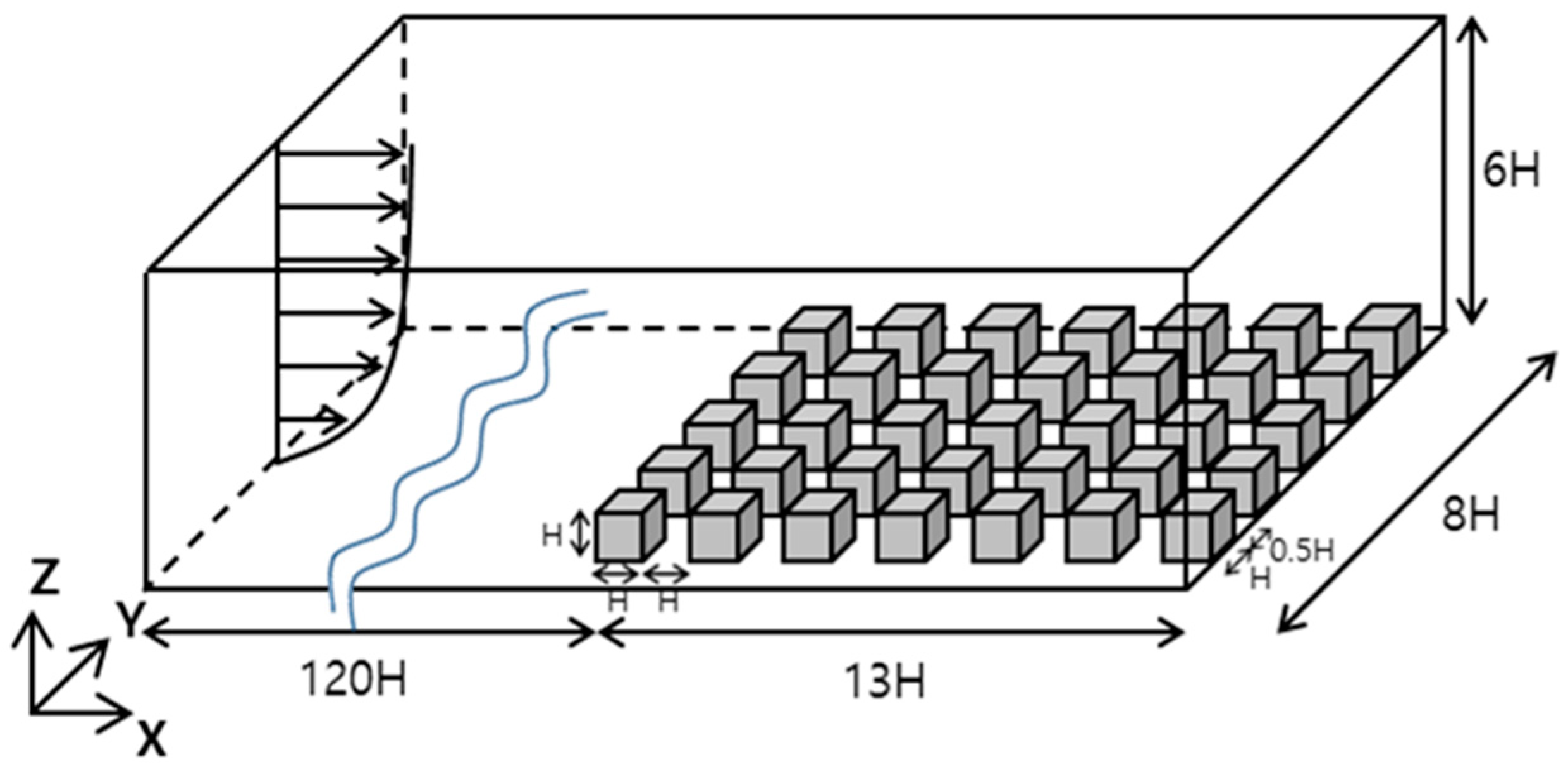
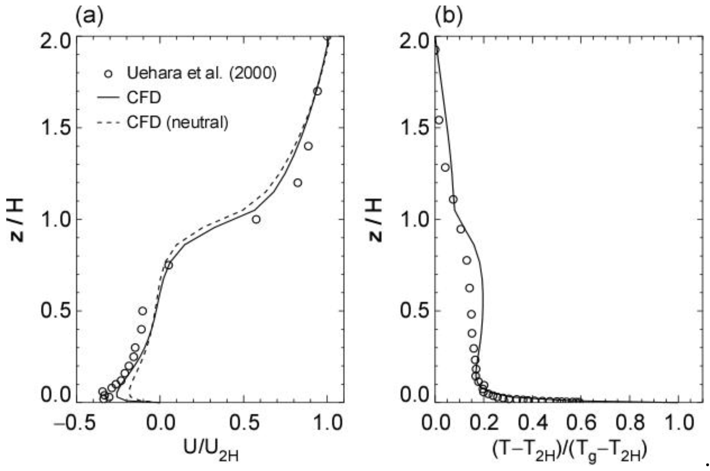
3.1. Validation of the CFD Model against Wind Tunnel Data

The CFD model of the new building-scale meteorological prediction system has been validated against the wind tunnel data of Uehara et al. [6] to investigate the performance of the CFD model in predicting atmospheric profiles of urban flow and air temperature. Uehara et al. [6] examined the effects of atmospheric stability on atmospheric flow in urban street canyons through the wind tunnel experiments with varying atmospheric stability, which measured atmospheric flow and temperature fields within and above the street canyon. The urban geometry was configured using building blocks with a size of 0.1 × 0.1 × 0.1 m³, which were arranged homogeneously with a spacing of 0.1 m in the x-direction and 0.05 m in the y-direction, respectively. Thus, the urban geometry parameters of H/W (building height/canyon width) and H/L (building height/canyon length) are 1.0 and 0.5, respectively. The urban geometry corresponds to the skimming flow regime [30]. The inflow turbulent boundary layer formed 7H in depth with a roughness length of 0.0033 m and a zero-plane displacement height of 0.035 m before impinging the array of the building blocks. The thermal forcing in the wind tunnel experiments was assigned with the air temperature of 20 °C and the surface temperature of 79 °C, which results in an unstable atmospheric condition with the bulk Richardson number of −0.21. The measurements were conducted between the fifth and sixth rows of the building blocks and the vertical sections of wind speed and temperature were taken at the center of the street canyon.

The domain of the CFD model was set identical to the wind tunnel experiment (Figure 2). The model domain has 13.3 m (x) × 0.8 m (y) × 0.6 m (z). The building blocks were resolved with a grid spacing of 0.01 m. The geometric and dynamic similarities were taken into consideration. The inflow flow condition was assigned using a power-law profile of $u\left(z\right)=u_{ref}{\left(\frac{z}{\mathrm{H}}\right)}^{0.16}$, where the reference wind speed ($u_{ref}$) was set to 3 m s⁻¹. With the constant wind profile, the turbulent boundary layer was developed for a patch distance of 12 m with the same surface roughness conditions of the wind tunnel experiment, and then the well-developed turbulent flow impinged the rows of building blocks. A zero-gradient condition was applied for the outflow and lateral boundary conditions. The atmospheric temperature and the ground surface temperature were set identical to the wind tunnel experiment, configuring the atmospheric stability of Ri = −0.21.

Figure 3 compares the measured and simulated mean wind and temperature profiles at the center of the street canyon. The mean wind profiles were normalized by the streamwise wind velocity at 2H and the temperature profiles were expressed by the temperature difference from the temperature at 2H normalized by the temperature difference between the ground (T_g) and the temperature at 2H (T_2H). It is observed that the approaching mechanical forcing formed a single vortex structure within the canyon and the sharp gradient just above the building block in the streamwise direction. The center height of the vortex is located at approximately 0.6H. In the neutral simulation, the observed primary vortex structure and the sharp vertical gradient were reasonably captured because the observed characteristics are primarily mechanically driven. The simulation with the unstable atmospheric stability compares against the wind tunnel data better than the neutral simulation, enhancing the in-canyon vortex intensity and the vertical gradient (Figure 3a). The improvement in the streamwise wind velocity is more clearly identified near the ground, which might be influential in predicting the pedestrian-level wind environments. It is also shown that the surface heating formed the characteristic temperature profiles that have a strong gradient near the ground (z/H < 0.1) and the well-mixed structure within the canyon (0.1 < z/H < 1.0). The temperatures gradually decrease above the building block (z/H > 1.0). The observed temperature profiles within and above the street canyon were well simulated by the CFD model (Figure 3b). This result indicates that the CFD model developed in this study is capable of predicting the atmospheric wind and temperature structures under neutral and unstable stability conditions.

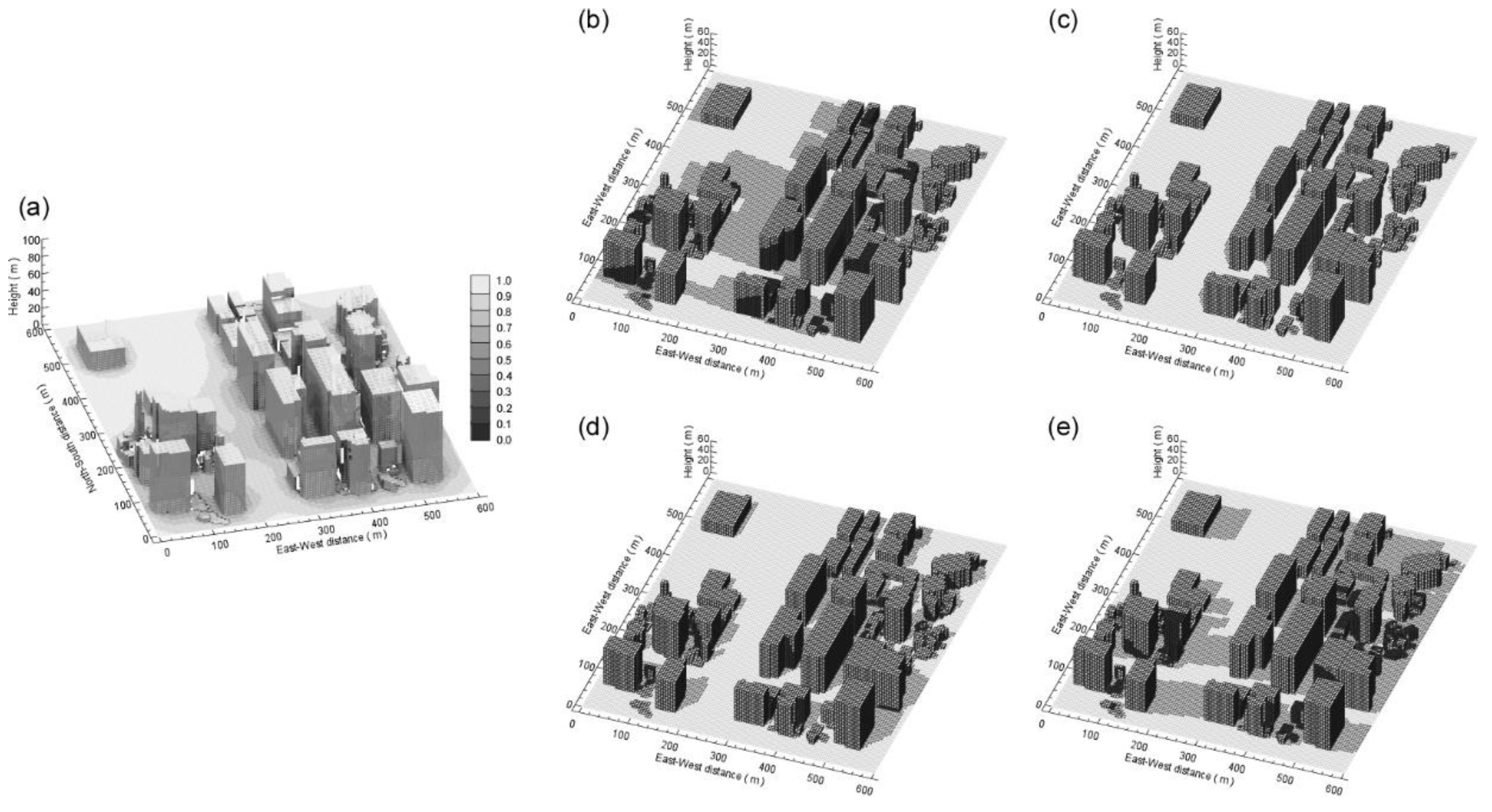
3.2. Validation of the MUSE Model against Field Measurements in a High-Rise Commercial Area

The MUSE model of the new building-scale meteorological prediction system has been validated against field measurements collected in a highly built-up real urban area. Many aspects associated with heterogeneous surface temperatures in real urban environments were considered for validation and meteorological simulation of the building-scale meteorological prediction system. A high-rise built-up area in Seoul, South Korea (37.572° E, 126.978° N) was selected for this study. The area can be characterized by a high dense commercial/residential area with high and low-rise buildings (Figure 4a). Various meteorological variables were continuously measured by the 3 dimensional sonic anemometer, thermometer, and infrared thermal imagery camera deployed at a 7-m meteorological tower on a building rooftop (71 m above the ground level) [8]. The simulation domain of the MUSE model was configured by 120 × 120 × 27 grid mesh with a horizontal and vertical spacing of 5 m and 3 m, respectively, covering the area of 600 (x) × 600 (y) × 81 (z) m³ surrounding the measurement tower (Figure 4b). The surface grid representation was used identically with the CFD model except that the vertical grid was stretched up to 300 m in meteorological simulations. The thermal properties of road and building surfaces were assigned with asphalt and concrete, respectively [31].

The simulation was conducted for a clear day of 7 September 2015 when weak easterly winds were dominant throughout the day. Figure 5 shows the diurnal variations of the radiative and meteorological forcing variables on the day. The downward shortwave and longwave radiation were obtained from the automatic surface observation station operated by the Korea Meteorological Administration (KMA), which is located about 1 km west. The downward longwave radiation was calculated from the observed atmospheric temperature and cloudiness at the site [31,32]. The atmospheric temperature, pressure, and wind were obtained from the tower measurements (Figure 5b). The vertical profiles of atmospheric temperature were assigned homogeneously, while the vertical wind profiles were modified using the wind fields of the neutral CFD simulation.

Figure 6 shows the spatial distributions of the sky-view factors and the building shadows on the simulation domain. The MUSE model in computing 3 dimensional view factors at every urban facet uses a simple numerical method by Lee et al. [17]. The sky-view factors at open ground and rooftop surfaces in the domain were estimated as high values around 1, while the values were relatively low in the narrow canyon ground. The vertical gradient of the sky-view factors on the wall surface of tall buildings is also reasonably represented (Figure 6a). The building shadows are determined by the relative position of the sun and buildings, thus they vary with time and space. The temporal variations of the solar zenith and azimuth angles were calculated in the MUSE model. The model well captured the diurnal variations of the sunlit and shaded areas in the real urban environment (Figure 6b–e), which changed significantly the incident shortwave radiation at each urban facet. The reasonable representation of the sky-view factors and the building shadow is important in calculating the radiative shortwave and longwave energy exchanges between the buildings.

Figure 7 shows the spatial distributions of the simulated surface temperatures at the wall and ground surfaces and the frequency distribution over the urban area during the day. The model simulated the heterogeneous distribution of the surface temperatures at different times of the day through the consideration of the surface energy balance of each urban facet. At 09 LST, the spatial variation of the wall ground surface temperatures was relatively small, approximately 20 °C, within the model domain (Figure 7a). As the downward shortwave radiation increased, the surface temperature of each urban facet gradually increased up to approximately 50 °C (Figure 7b–d). In addition, the spatial heterogeneity in the surface temperatures also significantly increased over 20 °C during the daytime (Figure 7e). The large spatial heterogeneity of the surface temperatures was primarily due to the difference in the incident direct shortwave radiation on each urban facet. This result showed that the realistic representation of the radiative energy exchanges was primarily important in determining the urban surface temperatures and forming thermal heterogeneity in the real urban environment.

Figure 8 compares the diurnal variations of the measured and simulated surface temperatures at the roof, wall, and ground surfaces. The surface temperatures at a ground (P1), east-facing walls (P2 and P4), and a north-facing wall (P3) were obtained from the infrared thermal imagery measurement at the meteorological tower site (Figure 8a). The roof surface temperatures, which were obtained from the infrared thermometer at the rooftop of the meteorological measurement tower site, varied 18–42 °C during the day with a very large diurnal range of 24 °C. The nocturnal surface temperatures were well simulated by the MUSE model, but the daytime surface temperatures were slightly underestimated (Figure 8b). The model well simulated the observed characteristic diurnal variations with a reasonable diurnal range at east-facing and north-facing wall surfaces, but it showed systematic cold biases at all the wall surfaces throughout the day (Figure 8c). The diurnal variation of the ground surface temperatures was well compared with the roof surface temperatures showing a slightly reduced diurnal range of 21 °C. The model simulated the observed diurnal variation of the road surface temperatures, but it slightly overestimated the observed diurnal range (Figure 8d). The model-measurement discrepancies might attribute to various factors such as thermal properties of the urban surfaces, uncertainties in the meteorological forcing and measurement, but it is difficult to separate the errors due to complex interactions of the urban physical processes in the real simulation. Despite the discrepancies, overall the validation results showed that the model represented well the spatial and temporal variations of the urban surface temperatures.

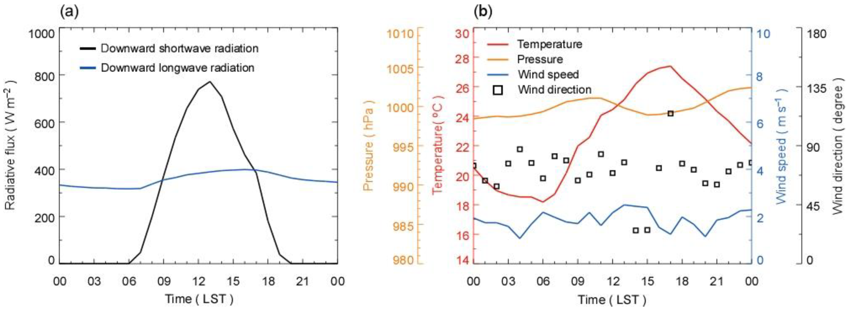
3.3. Validation of the Building-Scale Meteorological Prediction System against Field Measurement

The building-scale meteorological prediction system has been applied over the real urban area for the day of 7 September 2015, in which the surface temperatures predicted by the MUSE model were incorporated as a thermal bottom boundary conditions and the wind and temperature profiles operationally predicted by the LDAPS were used as a large scale meteorological forcing. The inflow profiles of turbulent kinetic energy and its dissipation rate were calculated with the roughness length and the boundary layer height of 0.1 m and 1000 m, respectively. The building-scale meteorological prediction system produced hourly microscale wind and temperature fields that are influenced by the realistic surface heating and the large scale meteorological forcing in the highly built-up urban area. Figure 9 compares the atmospheric temperature and wind fields simulated by the building-scale meteorological prediction system against the field measurements at the meteorological tower site. The operational forecast by the LDAPS was also compared to evaluate the potential performance of the new microscale model in simulating atmospheric temperature and wind fields over the urban area. The atmospheric temperatures measured at 78 m a.g.l. ranged from 16 °C at 06 LST to 26 °C at 17 LST, which were simulated better by the building-scale meteorological prediction system than the LDAPS especially during the daytime (Figure 9a). The improvement was largely attributed to the realistic representation of the urban surface temperatures shown in Figure 7. The low predicted atmospheric temperature at night might be largely attributed to the discrepancy in the LDAPS prediction. The measured wind speeds and directions ranged 1–3 m s⁻¹ and 60–90° (easterly) throughout the day, respectively (Figure 9b,c). The diurnal change in the measured wind direction was reasonably well simulated by both the models (Figure 9c). The LDAPS overestimated the measured wind speeds throughout the day, whereas the building-scale meteorological prediction system showed a better agreement with the measurement (Figure 9b). The better agreement of the wind speed in the building-scale meteorological prediction system might be attributed to the explicit representation of surface momentum drag of the real urban geometries, in which the pressure drag by buildings was predominant compared to the Reynolds stresses. Overall, the validation results showed that the new building-scale meteorological prediction model had a better capability than the LDAPS in simulating microscale meteorological fields in the highly built-up urban areas.

4. The Effects of Realistic Surface Heating on Pedestrian-Level Wind and Temperature Fields

Two sensitivity simulations with no surface heating and homogeneous surface heating have been further conducted for the built-up urban area using the building-scale meteorological prediction system to investigate the effects of the realistic surface heating on pedestrian level wind and thermal environments. The former simulation considered no surface heating at all urban facets within the domain and the latter simulation assigned the domain averaged surface temperature identically to all the urban facets at every hour (Figure 7e). All three simulations were conducted for 7 September 2015 with the same configuration except for the bottom thermal boundary conditions.

The wind velocity ratio (${\mathrm{V}}_{\mathrm{r}}$), which is commonly used in the ventilation studies (e.g., [33]), was used in the analysis of pedestrian-level wind environment, which is defined by

$${\mathrm{V}}_{\mathrm{r}}=V_p/V_{\infty }.$$

(13)

Here, $V_p$ is the wind speed at the pedestrian level and $V_{\infty }$ is the wind velocity just above the atmospheric boundary layer. In this study, $V_p$ and $V_{\infty }$ were used by the wind velocity at the first vertical grid level of 1.5 m and at 300 m above the ground level, respectively. The analyses of the realistic surface heating effects were investigated for the daytime period with enhanced thermal heterogeneity in the urban area.

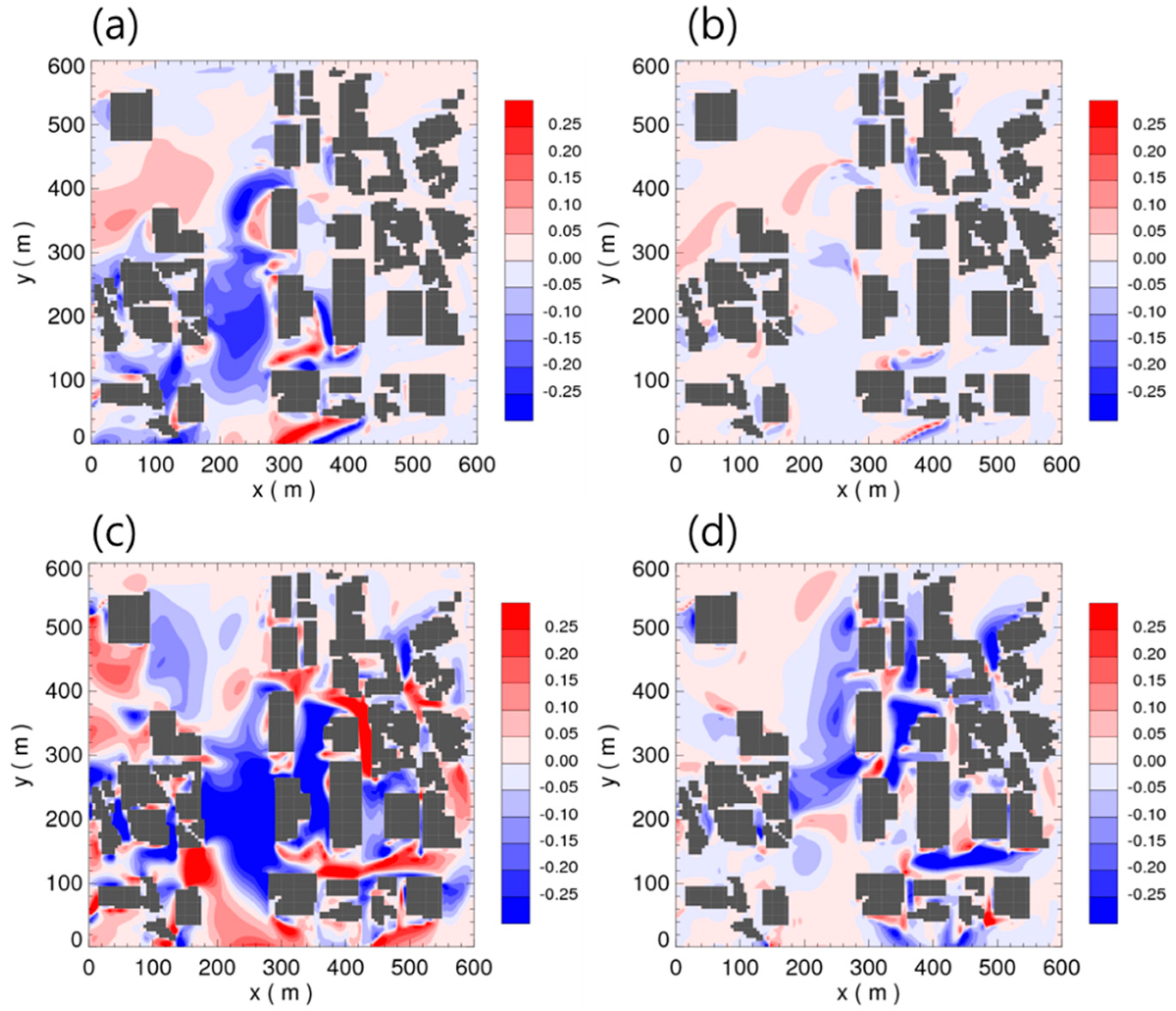
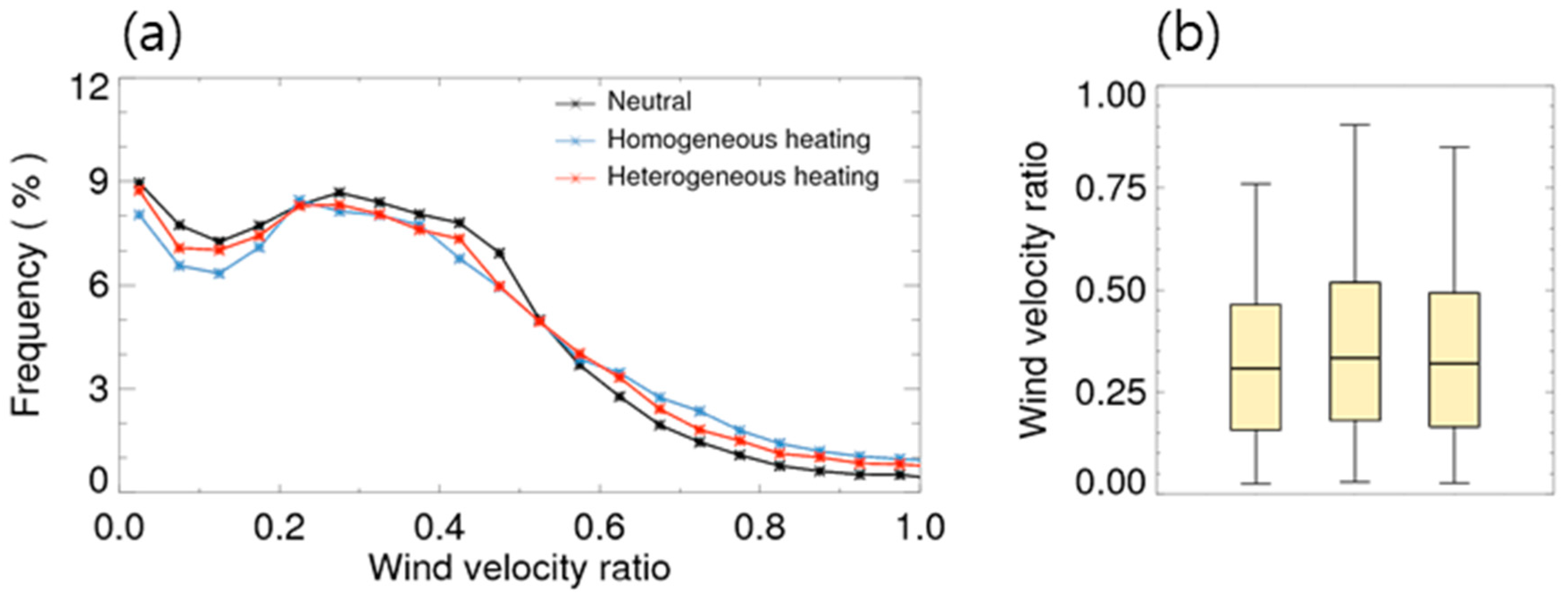
4.1. The Thermal Effects on Pedestrian-Level Wind Environment

Figure 10 compares the spatial distributions of the pedestrian-level wind field and wind velocity ratio in the highly built-up urban area simulated with the different surface heating conditions at 10 LST and 14 LST. At 10 LST, the large scale inflow wind direction and speed were approximately 60° and 4 m s⁻¹ (Figure 9), respectively, and the surface temperatures in the urban facets of the domain ranged 14.9–29.7 °C and 22.6 °C on average (Figure 7e). The simulated pedestrian-level wind fields showed very complicated variations depending on the thermal forcing as well as the buildings’ shape and their spatial arrangement (Figure 10a–c). It is found that that the spatial distributions in wind direction show better consistency among the three simulations than in wind speed, which is mainly attributed to the formation of channeling flows between the buildings and wake flows behind buildings. In addition, the thermal forcing also significantly modified the wind fields, especially in their directions. Wang and Ng [33] reported the enhanced variance of wind direction in unstable atmospheric conditions in their PALM simulation with homogeneous surface heat fluxes in Hong Kong. These characteristic urban flows were also reasonably simulated by the PALM model in the high-rise building district in Hong Kong [33,34]. At 14 LST, the large scale inflow slightly changed counter-clockwise with the wind direction and speed of approximately 30° (northeasterly) and 3 m s⁻¹ (Figure 9), respectively, and the surface temperatures and their spatial heterogeneity were significantly increased ranging 19.6–42.5 °C and 29.7 °C on average (Figure 7e). The slight change in large scale inflow direction and speed, compared to 10 LST, led to large differences both in the pedestrian-level wind direction and speed as a consequence of the changes in the characteristic urban flows (Figure 10d–f). The surface thermal forcing also led to large changes from the neutral simulation in the pedestrian-level wind direction and speed, which is more clearly identified in 14 LST than 10 LST following the increased thermal forcing.

Figure 11 shows the differences in the simulated pedestrian-level wind velocity ratio in the highly built-up urban area among the sensitivity simulations. The heterogeneous surface heating changed the spatial distribution of the wind velocity ratio within the built-up area ranging by −0.17–0.07 in 10 LST and by −0.31–0.17 in 14 LST. The air ventilation within the building blocks was overall enhanced on the domain through the inclusion of the realistic surface heating, but the changes are significantly dependent on specific locations of the area and the intensity of the surface thermal forcing (Figure 11a,c). When compared to the homogeneous heating simulation, the spatial heterogeneity in urban surface temperatures changed the wind velocity ratio within the built-up area ranging by −0.04–0.04 in 10 LST and by −0.16–0.05 in 14 LST. The relatively large difference in the wind velocity ratio at 14 LST is attributed to the strong spatial heterogeneity in the urban surface temperatures. Overall, these results indicate that it is important to resolve the realistic prediction of the urban surface temperatures in predicting wind fields and assessing ventilation at a specific location in real urban areas.

Figure 12 compares the simulated wind velocity ratio values in the highly built-up urban area from 10–16 LST. The wind velocity ratio was binned by 0.05 and the occurrence frequency of each bin over the urban area was compared among the three simulations. The surface heating decreased the simulated wind velocity ratio values in the lower ${\mathrm{V}}_{\mathrm{r}}$ classes less than 0.5, while it increased the values in the higher ${\mathrm{V}}_{\mathrm{r}}$ classes (Figure 12a). This is a similar result found in Wang and Ng [33] which showed the increased wind velocity ratio values in the higher ${\mathrm{V}}_{\mathrm{r}}$ classes greater than 0.2 over a dense urban district in Hong Kong. This study shows that the simulation with heterogeneous surface temperatures gives slightly lower thermal influences on the wind velocity ratio than the homogeneous surface heating, which is also shown in the statistical distributions (Figure 12b). The wind velocity ratio in the building district ranged 0.03–0.76 in the neutral simulation, 0.03–0.90 in the homogeneous simulation, and 0.03–0.85 in the heterogeneous simulation with a median wind velocity ratio of 0.31 in the neutral simulation, 0.33 in the homogeneous simulation, and 0.32 in the heterogeneous simulation.

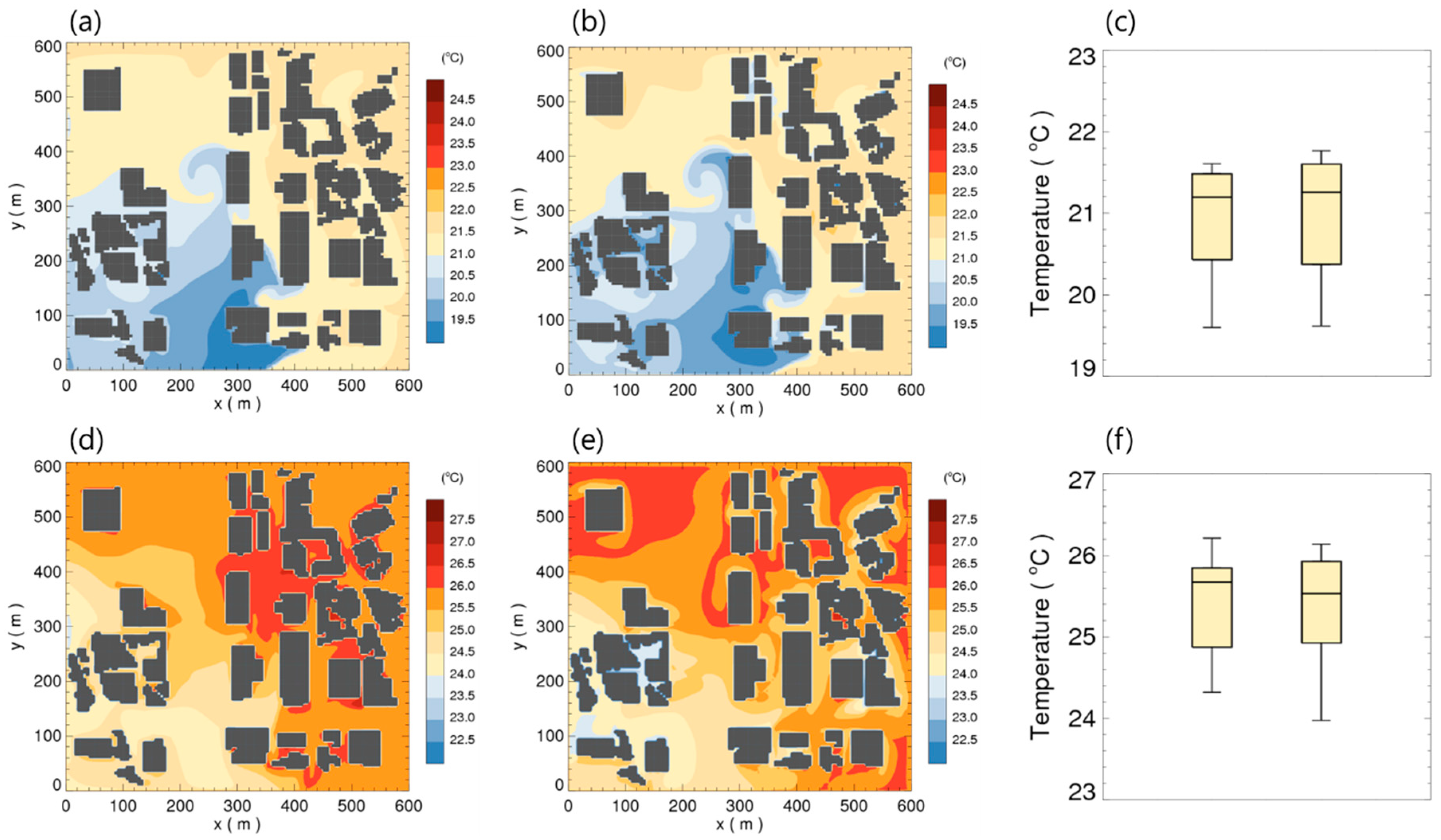
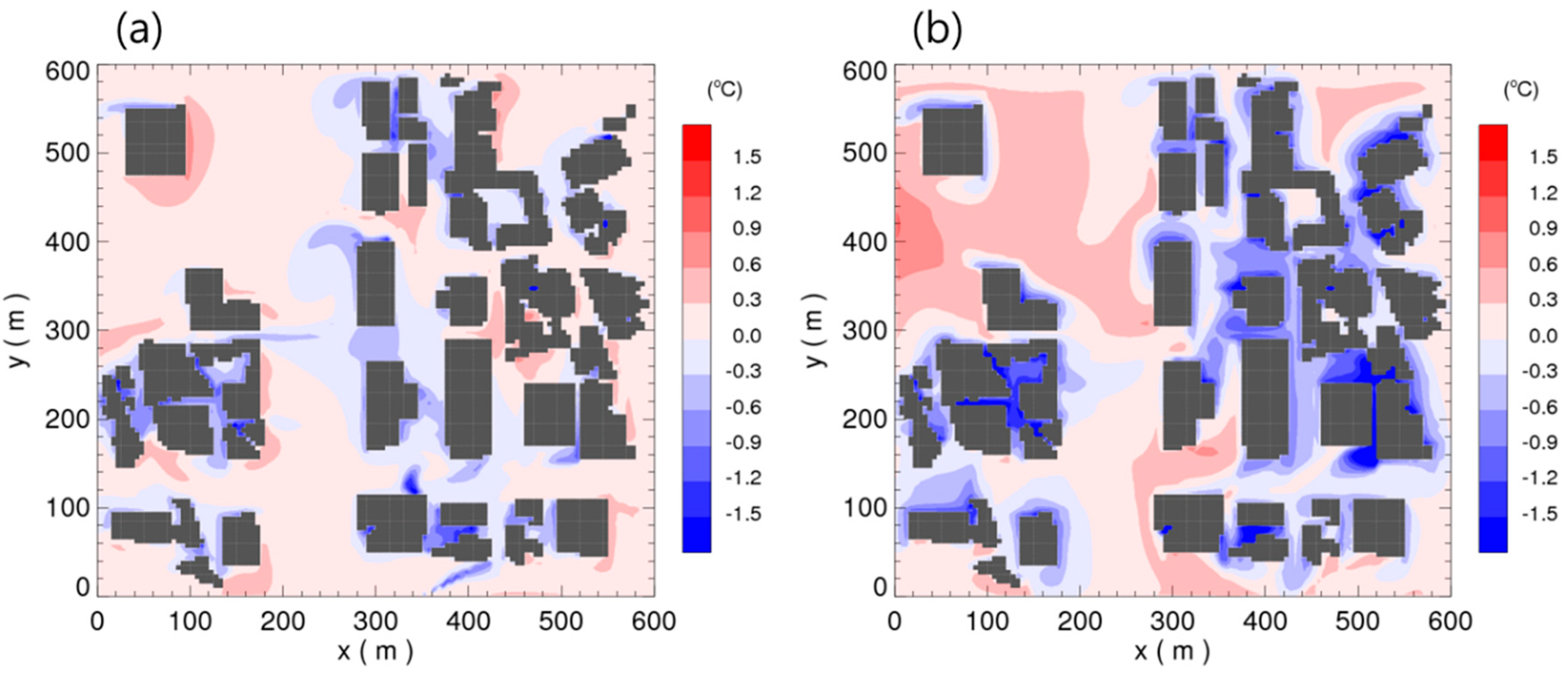
4.2. The Thermal Effects on Pedestrian-Level Thermal Environment

Figure 13 compares the spatial distributions of the pedestrian-level air temperature in the highly built-up urban area simulated with the homogeneous and heterogeneous surface heating conditions. The simulated pedestrian-level air temperatures ranged 19.6–21.8 °C at 10 LST and 24.0–26.1 °C at 14 LST, showing spatial variations of approximately 2 °C within the urban district (Figure 13b,e). The spatial variations in pedestrian-level air temperature are not resolved in the operational mesoscale weather forecast model of the LDAPS. Meanwhile, the simulated pedestrian-level air temperatures with heterogeneous surface heating were similar in statistical distribution within the urban district (Figure 13c,f). However, the spatial distribution of the simulated temperatures was quite different between the homogeneous and heterogeneous surface heating simulations, ranging −0.41–0.30 °C at 10 LST and −0.81–0.46 °C at 14 LST, respectively (Figure 14). Large differences in the pedestrian-level air temperature were found near the wall surfaces of the buildings, which indicates that accurate representation of the urban surface temperatures is important.

Overall, these results inferred that reasonable representation of both the urban mechanical and thermal forcing is a prerequisite in accurately predicting the pedestrian-level wind and thermal environments of the real urban area. The new building-scale meteorological prediction system well captured the characteristic urban flows (e.g., channeling flows between buildings and wake flows behind buildings) and the spatial variations of the pedestrian-level wind and air temperature fields in the highly built-up real urban area by virtue of the inclusion of the realistic surface heating by the MUSE, the explicit representation of mechanical forcing of buildings, and the large-scale meteorological forcing of the LDAPS into the CFD model.

5. Summary and Conclusions

Microscale urban meteorological models have been widely used in interpreting urban flow and thermal discomfort mostly under idealized urban morphological and physical environments. In this study, a new building-scale meteorological prediction system has been developed to extend the ability to predict microscale meteorological fields in real urban environments. A CFD model has been developed following Baik et al. [10], which solves the non-hydrostatic incompressible RANS equations with a standard k-ε turbulence model. The prognostic variables were discretized on the Arakawa-C grid system by a finite volume method in which the interpolation process was calculated by the power-law scheme. The new building-scale meteorological prediction system has been developed through a one-way coupling of the CFD model and the MUSE model, which is driven by the large scale wind and temperature fields predicted by the LDAPS/KMA. The MUSE model includes the urban physical parameterizations of building shadow effects, in-canyon direct and diffuse shortwave radiative transfer processes, turbulent sensible heat exchange processes between artificial surfaces and their surrounding atmosphere, and sub-surface thermal conduction processes, consequently being capable of predicting urban surface temperatures for real urban environments. The MUSE model provides realistic surface heating conditions for the CFD simulations in real urban environments.

The new building-scale meteorological prediction system was validated in its ability of canyon flow and thermal structure prediction against the wind tunnel data and field measurements obtained in a highly built-up urban area in Seoul, Korea. The results showed that the CFD model well captured the characteristic features of the measured in-canyon vertical temperature structure, showing the importance of surface heating. Additionally, the surface temperatures of different urban facets simulated by the MUSE model compared well against the IR imagery surface temperatures in the highly built-up urban area, highlighting the importance of the solar position and building morphology in urban surface temperature prediction. Overall, the validations showed its ability to predict in-canyon flows and thermal environments in association with spatial and temporal variations of urban surface temperatures in the real urban environment.

The effects of realistic surface heating on pedestrian level wind and thermal environments have been further investigated through three sensitivity simulations of no heating, homogeneous heating, and heterogeneous heating conditions in the highly built-up urban area for a clear day of 7 September 2015. The results showed that either of homogeneous or heterogeneous surface heating increased domain-mean pedestrian level wind speeds and their spatial heterogeneity compared to the neutral simulation, resulting in the higher frequency of high ${\mathrm{V}}_{\mathrm{r}}$ classes and the lower frequency of low ${\mathrm{V}}_{\mathrm{r}}$ classes. The change in mean air temperature was minor because the thermal forcing of the homogeneous heating case was assigned identically with a domain mean surface temperature. Meanwhile, a similar statistical frequency distribution was found both in the pedestrian level velocity ratio and the air temperature at the homogeneous and heterogeneous surface heating cases, even though the wind speed at each grid location has changed in time and space according to the thermal boundary conditions. These results imply that the inclusion of surface heating, as a forcing of microscale meteorological models, is important in interpreting urban flow and thermal comfort of a certain urban area in a statistical sense, for which homogeneous heating becomes a good assumption. However, it is identified that realistic urban surface heating should be considered in predicting building-scale meteorology over real urban environments. Most previous studies examined the urban flow, dispersion, and thermal discomfort of an urban area imposing neutral or homogeneous thermal forcing for an idealized urban morphology, this study highlights the importance of imposing realistic urban surface heating in microscale urban meteorological simulations. In this sense, the new building-scale meteorological prediction system developed in this study can be a useful tool for the evaluation and prediction of urban flow and thermal conditions for real urban environments.

More research is needed to evaluate and improve the building-scale meteorological prediction system. Intensive field measurements are necessary to evaluate the model’s capabilities faithfully in the real urban environment. In addition, a two-way coupling of the CFD model and the MUSE model will be able to provide a more realistic modeling strategy.

References

1. World Urbanization Prospects: The 2014 Revision, Highlights; United Nations: New York, NY, USA, 2014.
2. Oke, T.R. City size and the urban heat island. Atmos. Environ. 1973, 7, 769–779. [Google Scholar] [CrossRef]
3. Kim, H.-H. Urban heat island. Int. J. Remote Sens. 1992, 13, 2319–2336. [Google Scholar] [CrossRef]
4. Brown, M.J.; Lawson, R.E.; DeCroix, D.S.; Lee, R.L. Mean flow and turbulence measurements around a 2-D array of buildings in a wind tunnel. In Proceedings of the 11th Joint Conference on the Applications of Air Pollution Meteorology with the AWMA, Long Beach, CA, USA, 9–14 January 2000. [Google Scholar]
5. Brown, M.J.; Lawson, R.E.; DeCroix, D.S.; Lee, R.L. Comparison of centerline velocity measurements obtained around 2D and 3D building arrays in a wind tunnel. In Proceedings of the 2001 International Symposium on Environmental Hydraulics, Tempe, AZ, USA, 5–8 December 2001. [Google Scholar]
6. Uehara, K.; Murakami, S.; Oikawa, S.; Wakamatsu, S. Wind tunnel experiments on how thermal stratification affects flow in and above urban street canyons. Atmos. Environ. 2000, 34, 1553–1562. [Google Scholar] [CrossRef]
7. Allwine, K.J.; Leach, M.J.; Stockham, L.W.; Shinn, J.S.; Hosker, R.P.; Bowers, J.F.; Pace, J.C. Overview of Joint Urban 2003—An Atmospheric dispersion study in Oklahoma City. In Proceedings of the AMS Symposium on Planning, Nowcasting, and Forecasting in the Urban Zone, Seattle, WA, USA, 11–15 January 2004. [Google Scholar]
8. Park, M.-S.; Park, S.-H.; Chae, J.-H.; Choi, M.-H.; Song, Y.; Kang, M.; Roh, J.-W. High-resolution urban observation network for user-specific meteorological information service in the Seoul Metropolitan Area, South Korea. Atmos. Meas. Tech. 2017, 10, 1575–1594. [Google Scholar] [CrossRef]
9. Kim, J.-J.; Baik, J.-J. A numerical study of thermal effects on flow and pollutant dispersion in urban street canyons. J. Appl. Meteorol. 1999, 38, 1249–1261. [Google Scholar] [CrossRef]
10. Baik, J.-J.; Kim, J.-J.; Fernando, H.J. A CFD model for simulating urban flow and dispersion. J. Appl. Meteorol. 2003, 42, 1636–1648. [Google Scholar] [CrossRef]
11. Kwak, K.-H.; Baik, J.-J.; Lee, S.-H.; Ryu, Y.-H. Computational fluid dynamics modelling of the diurnal variation of flow in a street canyon. Bound.-Layer Meteorol. 2011, 141, 77. [Google Scholar] [CrossRef]
12. Park, S.-B.; Baik, J.-J.; Raasch, S.; Letzel, M.O. A large-eddy simulation study of thermal effects on turbulent flow and dispersion in and above a street canyon. J. Appl. Meteorol. Climatol. 2012, 51, 829–841. [Google Scholar] [CrossRef]
13. Santiago, J.L.; Krayenhoff, E.S.; Martilli, A. Flow simulations for simplified urban configurations with microscale distributions of surface thermal forcing. Urban Clim. 2014, 9, 115–133. [Google Scholar] [CrossRef]
14. Nazarian, N.; Kleissl, J. CFD simulation of an idealized urban environment: Thermal effects of geometrical characteristics and surface materials. Urban Clim. 2015, 12, 141–159. [Google Scholar] [CrossRef]
15. Nazarian, N.; Kleissl, J. Realistic solar heating in urban areas: Air exchange and street-canyon ventilation. Build. Environ. 2016, 95, 75–93. [Google Scholar] [CrossRef] [Green Version]
16. Resler, J.; Krc, P.; Belda, M.; Jurus, P.; Benesova, N.; Lopata, J.; Vlcek, O.; Damaskova, D.; Eben, K.; Derbek, P.; et al. PALM-USM v1.0: A new urban surface model integrated into the PALM large-eddy simulation model. Geosci. Model Dev. 2017, 10, 3635–3659. [Google Scholar] [CrossRef] [Green Version]
17. Lee, D.-I.; Woo, J.-W.; Lee, S.-H. An analytically based numerical method for computing view factors in real urban environments. Theor. Appl. Climatol. 2018, 131, 445–453. [Google Scholar] [CrossRef]
18. Gronemeier, T.; Raasch, S.; Ng, E. Effects of Unstable Stratification on Ventilation in Hong Kong. Atmosphere 2017, 8, 168. [Google Scholar] [CrossRef] [Green Version]
19. Toparlar, Y.; Blocken, B.; Maiheu, B.; Van Heijst, G.J.F. A review on the CFD analysis of urban microclimate. Renewable Sustainable Energy Rev. 2017, 80, 1613–1640. [Google Scholar] [CrossRef]
20. Wang, W.; Xu, Y.; Ng, E. Large-eddy simulations of pedestrian-level ventilation for assessing a satellite-based approach to urban geometry generation. Graph. Models 2018, 95, 29–41. [Google Scholar] [CrossRef]
21. Krayenhoff, E.S.; Voogt, J.A. A microscale three-dimensional urban energy balance model for studying surface temperatures. Bound.-Layer Meteorol. 2007, 123, 433–461. [Google Scholar] [CrossRef]
22. Zhang, Y.Q.; Arya, S.P.; Snyder, W.H. A comparison of numerical and physical modeling of stable atmospheric flow and dispersion around a cubical building. Atmos. Environ. 1996, 30, 1327–1345. [Google Scholar] [CrossRef]
23. Arya, S.P. Air Pollution Meteorology and Dispersion; Oxford University Press: New York, NY, USA, 1999; ISBN 978-01-9507-398-0. [Google Scholar]
24. Sini, J.-F.; Anquetin, S.; Mestayer, P.G. Pollutant dispersion and thermal effects in urban street canyons. Atmos. Environ. 1996, 30, 2659–2677. [Google Scholar] [CrossRef]
25. Patankar, S. Numerical Heat Transfer and Fluid Flow; CRC Press: Boca Raton, FL, USA, 1980; ISBN 978-08-9116-522-4. [Google Scholar]
26. Versteeg, H.K.; Malalasekera, W. An Introduction to Computational, Fluid Dynamics: The Finite Volume Method; Longman: Harlow, UK, 1995; ISBN 978-01-3127-498-3. [Google Scholar]
27. Launder, B.E.; Spalding, D.B. The numerical computation of turbulent flows. In Numerical Prediction of Flow, Heat Transfer, Turbulence and Combustion; Elsevier: Berlin, Germany, 1983; pp. 96–116. [Google Scholar]
28. Oke, T.R. The energetic basis of the urban heat island. Q. J. R. Meteorol. Soc. 1982, 108, 1–24. [Google Scholar] [CrossRef]
29. Lee, D.-I.; Lee, S.-H. A microscale urban surface energy (MUSE) model for real urban environments. Environ. Modell. Software. 2019, in press. [Google Scholar]
30. Oke, T.R. Street design and urban canopy layer climate. Energy Build. 1988, 11, 103–113. [Google Scholar] [CrossRef]
31. Lee, S.-H.; Park, S.-U. A vegetated urban canopy model for meteorological and environmental modelling. Bound.-Layer Meteorol. 2008, 126, 73–102. [Google Scholar] [CrossRef]
32. Swinbank, W.C. Long-wave radiation from clear skies. Q. J. R. Meteorol. Soc. 1963, 89, 339–348. [Google Scholar] [CrossRef]
33. Wang, W.; Ng, E. Air ventilation assessment under unstable atmospheric stratification—A comparative study for Hong Kong. Build. Environ. 2018, 130, 1–13. [Google Scholar] [CrossRef]
34. Letzel, M.O.; Helmke, C.; Ng, E.; An, X.; Lai, A.; Raasch, S. LES case study on pedestrian level ventilation in two neighbourhoods in Hong Kong. Meteorol. Z. 2012, 21, 575–589. [Google Scholar] [CrossRef]
Figure 1. Schematic diagram of the building-scale meteorological prediction system.
Atmosphere 11 00067 g001
Figure 2. Configuration of the computational fluid dynamics (CFD) computational domain and building blocks arrangement. H denotes the building height.
Atmosphere 11 00067 g002
Figure 3. Comparison of the simulated and measured (a) wind and (b) temperature profiles at the center of a street canyon.
Atmosphere 11 00067 g003
Figure 4. (a) The aerial photograph of a highly built-up urban area (“Gwangwhamoon”) in Seoul, South Korea and (b) the spatial distribution of the buildings represented for the CFD simulation. The rectangle area in (a) represents the CFD simulation domain and the solid circle denotes the location of the meteorological tower. The triangular area denotes the view angle of the infrared thermal imagery camera deployed at the rooftop of the building.
Atmosphere 11 00067 g004
Figure 5. Diurnal variations of (a) downward shortwave and longwave radiation and (b) meteorological forcing variables on 7 September 2015.
Atmosphere 11 00067 g005
Figure 6. The spatial distributions of (a) the sky-view factors at the wall and ground surfaces and the simulated shadow distributions at (b) 09 LST, (c) 12 LST, (d) 15 LST, and (e) 18 LST.
Atmosphere 11 00067 g006
Figure 7. The spatial distributions of simulated surface temperatures at (a) 09 LST, (b) 12 LST, (c) 15 LST, and (d) 18 LST and (e) the diurnal variation of the simulated surface temperature frequency distribution over the urban area.
Atmosphere 11 00067 g007
Figure 8. (a) The specific locations of the surface temperatures obtained from the infrared thermal imagery. P1: ground, P2 and P4: east-facing walls, P3: north-facing wall. (bd) The comparison of the measured and simulated surface temperatures at the (b) roof, (c) walls, and (d) ground surfaces.
Atmosphere 11 00067 g008
Figure 9. Comparison of the measured and simulated (a) air temperature, (b) wind speed, and (c) wind direction at 78 m above the ground level.
Atmosphere 11 00067 g009
Figure 10. The spatial distributions of the simulated pedestrian-level wind fields with (a,d) no surface heating (neutral case), (b,e) homogeneous surface heating, and (c,f) heterogeneous surface heating. The upper and lower panels denote the results at 10 LST and 14 LST, respectively. The 1.5 m wind fields were plotted with arrows and the wind velocity ratio was denoted by the shaded contour.
Atmosphere 11 00067 g010
Figure 11. The spatial distributions of the simulated wind velocity ratio differences of the heterogeneous surface heating simulation from (a,c) the neutral case and (b,d) the homogeneous surface heating cases. The upper and lower panels denote the results at 10 LST and 14 LST, respectively.
Atmosphere 11 00067 g011
Figure 12. The comparison of the wind velocity ratio values simulated with no surface heating, homogeneous surface heating, and heterogeneous surface heating in (a) frequency distribution and (b) boxplot (left: no surface heating, middle: homogeneous surface heating, right: heterogeneous surface heating). The simulation results of 10–16 LST were analyzed in the plots.
Atmosphere 11 00067 g012
Figure 13. The spatial distributions of the pedestrian-level air temperatures simulated with (a,d) homogeneous surface heating, (b,e) heterogeneous surface heating, and (c,f) their difference at 10 LST (upper panels) and 14 LST (lower panels).
Atmosphere 11 00067 g013
Figure 14. The spatial distributions of the pedestrian-level air temperature difference between the homogeneous and heterogeneous surface heating cases at (a) 10 LST and (b) 14 LST.
Atmosphere 11 00067 g014