Article

Sensitivity Studies for a Hybrid Numerical–Statistical Short-Term Wind and Gust Forecast at Three Locations in the Basque Country (Spain)

by
Sheila Carreno-Madinabeitia
1,2,*,
Gabriel Ibarra-Berastegi
3,4,
Jon Sáenz
2,4,
Eduardo Zorita
5 and
Alain Ulazia
6
1
TECNALIA, Parque Tecnológico de Álava, Albert Einstein 28, E-01510 Vitoria-Gasteiz (Araba/Álava), Spain
2
Applied Physics II Department, Faculty of Science and Technology, University of the Basque Country, E-48940 Leioa, Spain
3
NE and Fluid Mechanics Department, Faculty of Engineering, University of the Basque Country, E-48013 Bilbao, Spain
4
Joint Research Unit, BEGIK, Spanish Institute of Oceanography-University of the Basque Country, Plentzia Itsas Estazioa (PIE), E-48620 Plentzia, Spain
5
Institute of Coastal Research, Helmholtz-Zentrum-Geesthacht, 21502 Geesthacht, Germany
6
NE and Fluid Mechanics Department, Faculty of Engineering, University of the Basque Country, E-20600 Eibar, Spain
*
Author to whom correspondence should be addressed.
Atmosphere 2020, 11(1), 45; https://doi.org/10.3390/atmos11010045
Submission received: 28 November 2019 / Revised: 24 December 2019 / Accepted: 27 December 2019 / Published: 29 December 2019
(This article belongs to the Section Atmospheric Techniques, Instruments, and Modeling)

Abstract

:
This study evaluates the performance of statistical models applied to the output of numerical models for short-term (1–24 h) hourly wind forecasts at three locations in the Basque Country. The target variables are horizontal wind components and the maximum wind gust at 3 h intervals. Statistical approaches such as persistence, analogues, linear regression, and random forest (RF) are used. The verification statistics used are coefficient of determination (R2) and root mean square error (RMSE). Statistical models use three inputs: (1) Local wind observations; (2) extended EOFs (empirical orthogonal functions) derived from past local observations and ERA-Interim variables in a previous 24-h period covering a domain around the area of study; and (3) wind forecasts provided by ERA-Interim. Results indicate that, for horizons less than 1–4 h, persistence is the best model. For longer predictions, RF provides the best forecasts. For horizontal components at 4–24 h horizons, RF slightly outperformed ERA-Interim wind forecasts. For gust, RF performs better than ERA-Interim for all the horizons. Persistence is the most influential factor for 2–5 h. Beyond this horizon, predictors from the ERA-Interim wind forecasts led the contribution. Hybrid numerical–statistical methods can be used to improve short-term wind forecasts.

1. Introduction

Providing accurate short-term wind prediction is an important goal for any meteorological service [1]. Wind storms in Spain produce important economic losses, representing 15% of all natural hazards damage compensations reimbursed by insurance companies from 1987 to 2015 [2]. A robust wind forecasting system must issue reliable warnings hours before potentially dangerous events occur, such as the windstorm Klaus [3]. Better short-term wind forecasts contribute to reducing economic damage and help save lives [4]. Reliable wind forecasts find many applications, including air pollution [5], wind power [6,7,8,9,10,11,12,13], forest fires [14], sea navigation [15,16], and airports [17,18].
Wind predictions are issued based on meteorological numerical weather forecast (NWF) systems, in which data assimilation (DA) plays an important role in order to properly correct errors in the forecasting model by the use of observations in the data assimilation stages. In these NWF systems, the data assimilation methods optimally estimate the state of the atmosphere [19,20] and a numerical weather forecast model is used to predict the future states of the atmosphere. Two examples of these advanced NWP systems are the ERA-Interim [21] global atmospheric reanalysis model, from 1979 until 2019 [21], and NCEP re-analyses [22]. They are not real-time operational NWF systems, since the DA and the forecasting models are frozen in time, but they are re-run for the whole period using all the available observations commonly used in numerical weather forecasts in order to avoid, as much as possible, errors in the record due to changes in the structure (architecture, resolution, kind of observations processed) of the archives derived from operational NWF systems. In the case of the ERA-Interim re-analyses, besides analyses, forecasts are also provided starting at the analysis times. These forecasts are the ones used in this paper as a surrogate of an operational model. However, re-analyses are quite coarse-resolution models when compared with operational models of the same generation. In the particular case of the ERA-Interim, the spatial resolution is 0.75°, too coarse for local wind forecasts.
To fill this resolution gap, numerical and statistical downscaling techniques are customarily used. Numerical downscaling increases the resolution by nesting a higher-resolution model, such as WRF [23], RAMS [24], or Hirlam [25], into the global NWF. Statistical downscaling, as an alternative downscaling method, uses transfer functions from predictors provided by low-resolution models to local predictands, as in Valero et al. [26], who used ERA-Interim data followed by an analogue downscaling method. Interesting results were obtained by Pascual et al. [27] using ECMWF’s ERA 40. Wind forecasts for horizons between a few hours to some days often involve the application of statistical post-processing to NWF model outputs. Global forecast system (GFS) [28], North American mesoscale forecast system (NAM) [29], and rapid update cycle (RUC) [30] NWF outputs were used, followed by statistical analogues post-processing in Nagarajan et al. [31]. In particular, in that paper, the objective was to forecast wind speeds at 6 h intervals up to 72 h horizons. Another example is Cassola and Burlando [8], where the BOLAM numerical model [32] was used, along with Kalman filter-based post-processing for forecasting wind speed for a horizon of up to 36 h at 6 h steps. A combined approach (GFS plus statistical downscaling) can also be found in other studies, such as Zhao et al. [33], where hourly averaged wind speed was predicted for 24 h horizons. A meteorological model like WRF [23], followed by analogues and Bayesian inference, was also used in complex terrain by Manor and Berkovic [34]. In this context, the Greek National meteorological service model (GNMS) applies locally recurrent neural networks [9] for hourly averaged wind speed with a 72 h horizon every hour. A study involving the same geographical area as this study [18] combined the forecasts by a global GFS model with a post-processing stage based on machine-learning techniques. The second stage, which used random forest (RF) amongst other methods, improved the quality of the raw forecast provided by the global NWF model. These results will be extended to different areas (ocean, coast, interior) in this contribution. Gust predictions are also of interest. Valero et al. [26] proposed a daily forecast derived from ERA-Interim by means of the analogue technique. Patlakas et al. [35] used the SKIRON/Dust [36] model, followed by Kalman Filter-based post-processing. Finally, Zjavka [37] predicted hourly gusts with the ALADIN model [38], using the polynomial neural networks technique. Statistical downscaling models in this context are calibrated with past observations and are later used to forecast future meteorological events. This is usually highly site-dependent, because the model structure and parameters are specifically developed for the location [8,34,39,40,41,42].
For very short horizons (a few hours in advance) time-series based statistical models are commonly used. For example, hourly averaged wind forecasts have been issued by statistical models such as support vector regression (SVR) and artificial neural networks (ANN) [10,43,44]. Also, ARIMA models [41] were used to predict average wind speed. The authors of [45,46] developed a method that makes use of regime-switching for forecast wind speed hourly 12 h ahead. This way, they deal with non-stationarity in wind dynamics. A comparison of machine learning models for forecasting wind during the next hour was presented by Feng et al. [11]. Along these lines, ARIMA-ANN and ARIMA-Kalman Filter models have also been used [47] for 3 h forecasting. Hourly observations were used as target variables with ANN and genetic expression programming (GEP) [48]. A method similar to analogues [49] was also applied to forecast wind speed in the next hour [50]. Even [51] monthly mean wind speed has been forecasted combining time-series with ANN.
In summary, long-term (beyond a few days) forecasts are commonly issued by means of a global NWF followed by statistical post-processing [7]. While for time horizons of a few hours, forecast time-series based statistical models are usually applied, we propose to use both approaches in a hybrid wind forecast system.
Thus, we follow the well-stablished technique of testing the hybrid numerical–statistical methods by using data from a frozen assimilation system. This allows us to perform a sensitivity study of the relative merits of different statistical techniques under controlled conditions without introducing spurious modifications into the results due to changes in the configuration of the operational NWF system [8,18,26,27,31,33,39,52].
A comparison of more than 14 studies based on statistical methods for wind forecasting can be found in Okumus and Dinler [12] and references therein. As mentioned in that review, these kinds of wind-forecasting studies are sometimes difficult to compare. The root mean square error (RMSE) and the coefficient of determination (R2) are widely used in this field of research [8,18,26,27,31,33,42]. The main advantage of using R2 over the plain correlation is that the coefficient of determination is an indicator that represents the fraction of the overall variability explained by the model. A complete evaluation requires additional information on the error, either expressed in absolute terms (RMSE) or in percentage terms.
For this study, hybrid models were constructed using local observations and ERA-Interim data for short-term forecasting of wind speed and wind gust up to 24 h in the future at three selected locations in the Basque Country during 2007–2014 (Figure 1). The statistical algorithms used were analogues, linear regression, and random forest (RF). They are here applied to locations over the ocean, the coast, and the interior (see Figure 1).
Taking into account the results in aforementioned studies, our objectives were: First, a comparison of the performance of different hybrid numerical–statistical techniques in the forecasting of u and v components for three observatories located in the ocean, at the coast, and in the interior of the Basque Country in the Bay of Biscay. Secondly, a comparison of the performance of the best statistical model with two reference forecasts, the nearest grid cell direct model output from the coarse-scale NWF model, which provided the predictors and persistence. The rationale behind the use of these reference models (ERA-Interim and persistence) is that any forecasting effort for a certain number of hours in the future is justified only if the new model outperforms existing ones. The comparison of performances is presented both for hourly wind data and wind gusts. The robustness of the method is evaluated against the selection of the domain and by applying it to three different sites which present different wind regimes. Finally, the most significant predictors are also identified.
Section 2 presents the datasets and method used in this study. Section 3 describes the results, Section 4 discusses the conclusions of this study, and Section 5 presents a discussion along with a future outlook.

2. Material and Methods
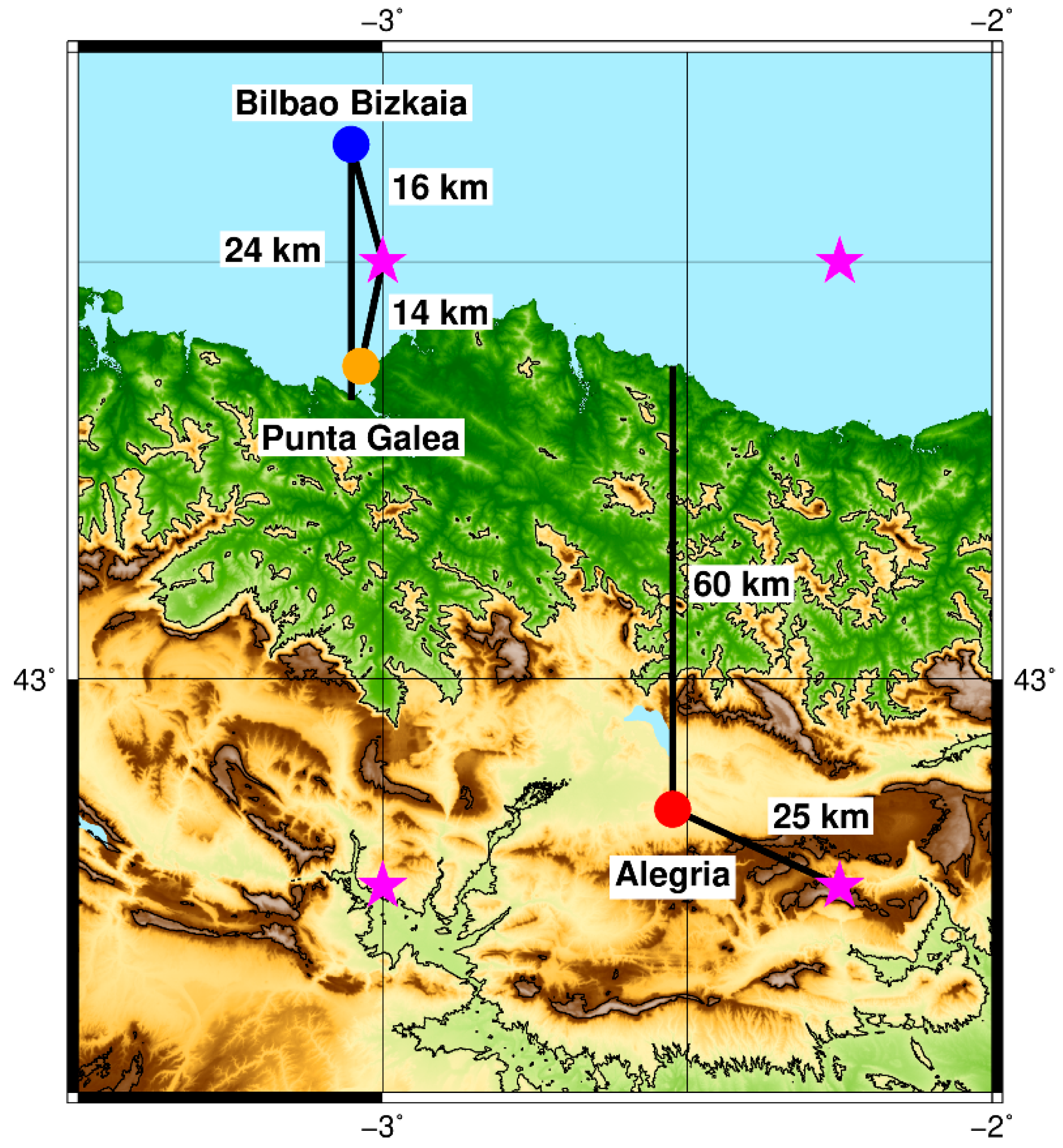
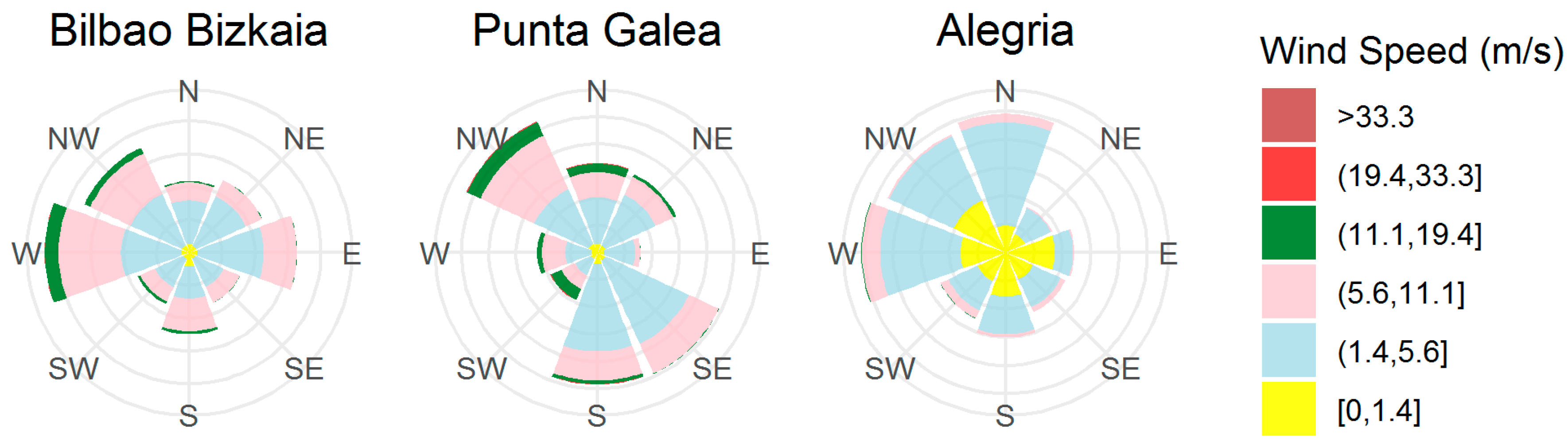
2.1. Data

The Basque country is located in the Bay of Biscay, an area with elevations that may reach 1000 m just 30 km away from the coast. The topographic gradient is moderately steep, and the wind regime is subject to important coastal influences. Thus, three locations are chosen for this study (Figure 1). They represent ocean, coastal, and interior wind regimes, as can be seen in their wind roses (Figure 2). One of them is a buoy (Bilbao Bizkaia), representing an oceanic regime. The other two sites were selected to compare the results of the sea with the coast and an inland zone in the area of interest.
The Bilbao Bizkaia buoy (43.64° N, 3.05° W) is run by the Spanish Puertos del Estado agency [53] and is located offshore, approximately 30 km from the coast. As can be seen from the wind roses, it is not affected by sea breezes and, since there are no natural obstacles around it, the wind tends to flow freely. The second location is Punta Galea, at the coastline, at the top of a cliff (43.38° N and 3.04° W, 61 m elevation above sea level). Punta Galea is exposed to sea–land interactions affecting the wind regime, such as sea breezes. The third wind sensor is located in Alegria, on a plateau in the south of the Basque Country (42.84° N and 2.52° W, 545 m elevation), 60 km inland. The dominant wind pattern is west–east but the highest wind corresponds to a south–west direction. Both inland stations are run by the Basque Meteorological Service (Euskalmet).
At each location, u, v, and wind gust at the sensor height above ground level (Bilbao Bizkaia: 3 m, Punta Galea: 12 m, and Alegria: 10 m) are measured. u and v were calculated using only the last measurements (10 min) prior to the hourly time step at the three locations. These are the operational averages regularly implemented and subsequently made public by the institutions running the sensors. The zonal (u) and meridional (v) projections of the wind vector were obtained from magnitude and direction recorded at the three locations.
A second group of target variables was used at the three locations: Hourly maximum wind gusts. The wind gusts were computed from the maximum value of the gust recorded in the last 10 min at Punta Galea and Alegria. The maximum value for the Bilbao Bizkaia buoy was calculated using the measurements taken over the last 10 min of each hourly step because the buoy records data every hour while the meteorological stations do this every 10 min. Only the magnitude of wind gust was used. To compare the data with the ERA-Interim forecast, the wind gust since previous post-processing (3 h period) was calculated; this will hereinafter be referred to simply as wind gust. All the data span the period 2007–2014.
Data from ECMWF’s ERA-Interim reanalysis [21,54] were used. The variables selected as likely to impact upcoming wind speed were mean sea level pressure (Msl); the zonal component of wind at 10 m (m/s) (u10); the meridional component of wind at 10 m (v10); and temperature at 2 m (T2). The domain selected (Figure 3) is a rectangle spanning (49.50° N, 12° W) to (36° N, 7.5° E) with a spatial resolution of 0.75° × 0.75°. Analyses at 6 h time steps for the 2007–2014 period were downloaded from ECMWF. Additionally, u10 and v10 and wind gusts in forecast mode from ERA-Interim for the nearest grid points from the three chosen locations were also used. From the initial conditions at t = 0000 UTC and t = 1200 UTC, ERA-Interim forecasts of these variables are available for t + k, where k = (3, 6, 9, 12, 15, 18, 21, 24) h in the future in the meteorological archival and retrieval system (MARS) server of the ECMWF. All these variables were used to feed the different wind forecasting models as if the statistical models were using forecasts from an operational model.

2.2. Method

In order to achieve a rigorous evaluation of the performance of statistical models, the original database was split into two datasets, one to fit and train the models (2007–2010) and the other to test the models on independent data (2011–2014). RF uses train and test datasets [18,55]; this method does not require validation datasets, such as the neural network method. The number of cases is shown in Table 1.
The raw input data were pre-processed as follows. At a given t time, each model at the different lead times was fed with:
  • Observations of u and v, and the wind gust at each sensor height when t = 0;
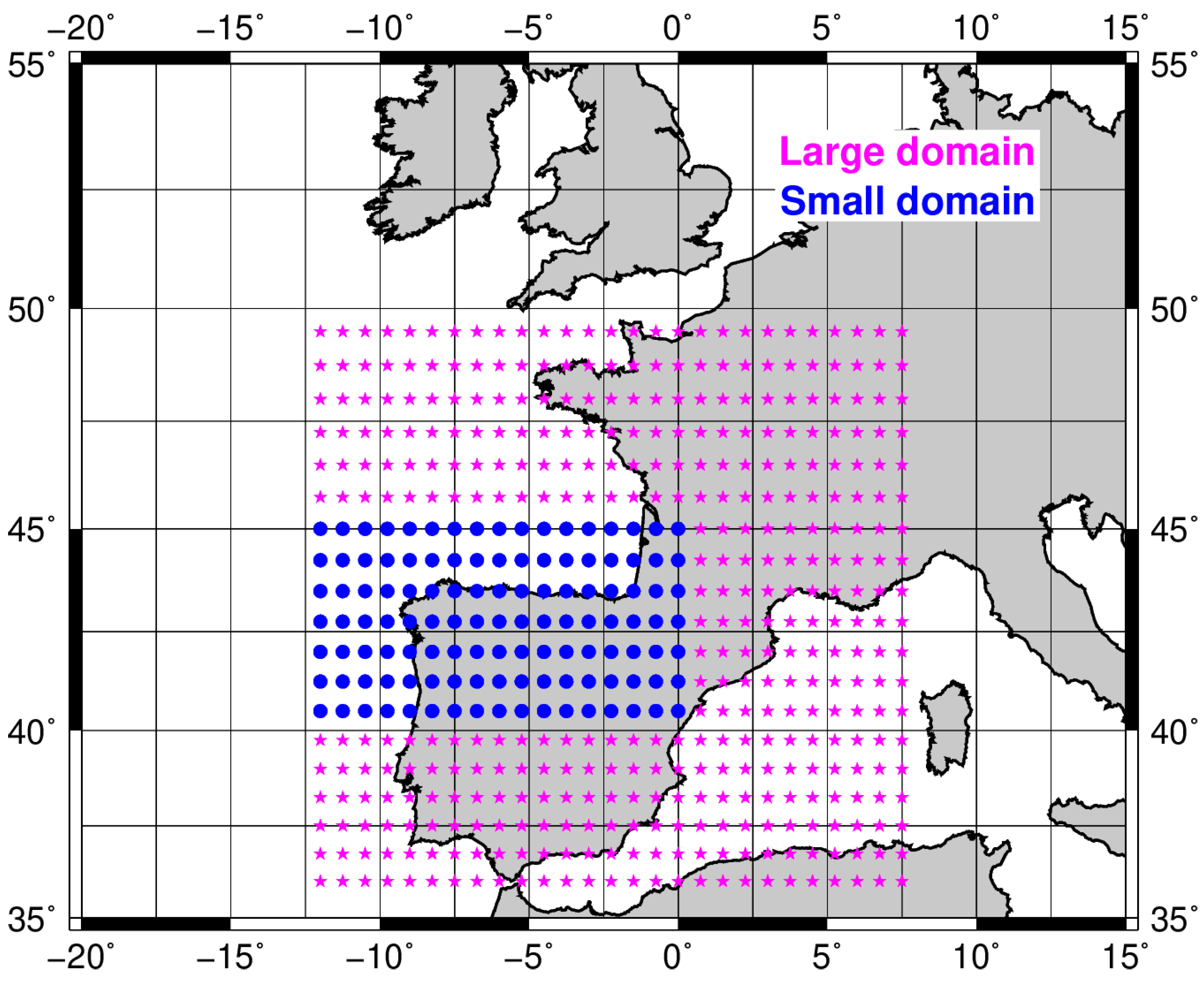
  • ERA-Interim forecasts (u, v, wind gust) for the nearest grid points from the selected locations (Figure 1). This NWF is based on a four-dimensional variational assimilation analysis, with a time window of 12 h, and produces forecasts with time steps that range from 3 to 24 h in the future, as explained in Section 2.1;
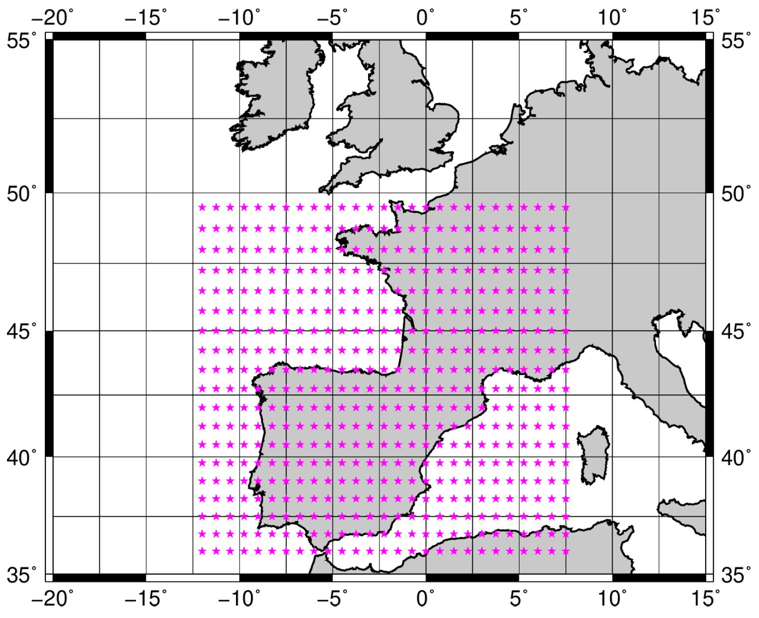
  • Time-lagged wind observation at t − 0, t − 6, t − 12, and t − 18 h. Time-lagged observations and ERA-Interim analyses (see domain in Figure 3) were used. In order to reduce the dimensionality of the time-lagged ERA-Interim variables (Msl, u10, v10, and T2), extended empirical orthogonal functions (extEOFs) of the original variables were calculated [56,57]. In this way, both spatial and temporal patterns can be captured in the space corresponding to the principal components, and the leading extEOFs hold the highest fractions of the total variance. The resulting extended principal components have not been rotated, since they were just used for compressing the information and they are, therefore, orthogonal. Extended EOFs have been applied, dealing with different geophysical variables, such as waves [52,58], ENSO events [59], and surface moisture flux and precipitation [55]. In the case of this study, important associations (correlations) were detected between variables, in addition to non-negligible autocorrelations and spatial correlations throughout the selected spatial and time domain. Due to the different physical quantities (K, m/s and so on) of the variables involved, at an initial stage they were standardized (mean = 0, variance = 1), and the final number of leading extEOFs used for this study was 26, selected under the condition of jointly retaining at least 90% of the overall variance, following the final criteria developed by authors for similar geophysical studies after careful evaluation of different alternatives [52,55].
A summary of the raw input data is shown below (Table 2).
Three statistical techniques were used: Analogues, linear regression, and RF. Linear regression is a common method in statistical prediction. Second, the analogues method is a non-linear technique that has been often used since the early days of meteorological forecasting [49]. The third technique was random forests (RF), a machine learning technique that we wished to compare with the two other, simpler methods.
For each target variable and statistical technique, a specific model was built for each of the forecasting horizons at t + k (k = 1, 2, …, 24) h. This means that, for u and v, a total of 432 models were constructed (two target variables times three locations times three techniques times 24 hourly steps). In the case of the wind gust, only the best technique identified for u and v was used RF. For wind gust, 72 models (one target variable times three locations times one technique times 24 hourly steps) were built. As a result, for this study, a total number of 504 models were developed and evaluated.
In the analogue technique [49], for each case in the test period, the most similar situation is sought in the training period and this becomes the wind prediction at t + h hours. Patterns can be selected using various similarity metrics [60], and, for this study, both Euclidean and cosine norms were applied. Given the state of the predictors to be used by the vector x = (x1, …, xp) with p the dimension of the state-space, the Euclidean distance between vectors x and y is defined by:
d ( x , y ) = | | x   y | | = i = 1 p ( x i y i ) 2
whilst the cosine distance is defined by:
d ( x , y ) = | | x y | | = i = 1 p x i y i   i = 1 p x i 2   i = 1 p y i 2
Random forest is a predictive algorithm that uses bootstrap technique to combine different decision trees, where each tree is built with observation data and random variables. RF [61] was considered due to its ability to mathematically capture highly non-linear relationships, like those known to be involved in the physics of wind forecasting. RF is a development of classification and regression trees (CART [62]), where the regression trees are randomly perturbed and a forest of perturbed trees is created. Trees are perturbed at two levels:
  • A number of bootstrap samples from original data are drawn and used to feed the different regression trees;
  • At each tree, each node is split using the best among a subset of m predictors randomly chosen at that node.
A key advantage of RF over other regression techniques is that it is free from overfitting, due to the use of the strong law of large numbers [61]. In RF, it is possible to estimate how important a given input is by calculating its percentage increase in the mean square error of the regression, if that particular predictor, is removed. This ranks the most influential inputs [63]. For this work, this importance ranking was estimated from the training dataset and, following the general procedure, the RF outputs were estimated as the average of the outputs of the trees [64,65].
In the case of the classical multiple linear regression, the candidate input variables are incorporated into the equation following the Akaike information criterion (AIC) [66]. Performance comparison for other atmospheric fields indicates that non-linear algorithms like neural networks outperform, but not overwhelmingly so, more simple methods like linear regression [67] and analogues [49,68]. RF is perhaps more difficult to implement than analogues or linear regression, but it has been successfully employed in other studies [55,69,70]. In particular, for the variable studied here—wind—[18] RF was used, as well as other machine learning techniques, to forecast wind speed. This latter study is the most similar to ours, because both forecast wind for same locations and used NWF model predictors for the statistical models. Details on most mathematical aspects of RF can be found in the literature [61,71]. For comparison purposes, in addition to the abovementioned models, the plain forecasts provided by ERA-Interim for time t + k (k = 3 h, 6 h, 9 h, …, 24 h), as well as persistence were also considered as additional models for each location and forecasting horizon.
Forecast accuracy was evaluated against observations exclusively using data belonging to the test period. The number of cases ranges from 1896 to 2231 (Table 1). The performance assessment was carried out by means of the usual indicators typically employed in the literature: R2 and RMSE [18,26,42,72]. In this study, a given model will be considered superior to another if both indicators, at a 95% confidence level, are better. All the comparisons using these indicators were assessed at a 95% confidence level using boundaries computed by bootstrap resampling [73]. In the process of selecting bootstrap samples, the time order of the series was taken into account.

3. Results

3.1. Model Performance for u and v

First, in this section, the results of three statistical models (linear regression, analogues, and RF) have been shown and compared for u and v targets. Then, the best result has been compared against persistence and ERA-Interim forecasts. The sensitivity to the domain size is also verified and finally the relevant inputs are identified.

3.1.1. Statistical Models

The forecasts by the three statistical models (linear regression, analogues, and RF) were compared in order to clarify which technique performed better. The goal was to identify the best general technique.
The results of this analysis are summarized in Table 3 and Table 4 and Figure 4. These tables and figure show a performance comparison for the statistical models built using the three techniques mentioned above. It can be seen that models based on RF, analogues, and linear regression tend to perform similarly for all the forecasting horizons (1 h, 2 h, …, 24 h) and only marginal—though statistically significant—improvements can be detected, depending on the location and forecasting horizons. In the case of one location (Bilbao Bizkaia), linear regression-based models performed slightly better for more forecasting horizons, while RF-based models exhibited a marginal improvement in the case of Punta Galea and Alegria. So, in general terms, RF-based models appear to perform best at the three locations.

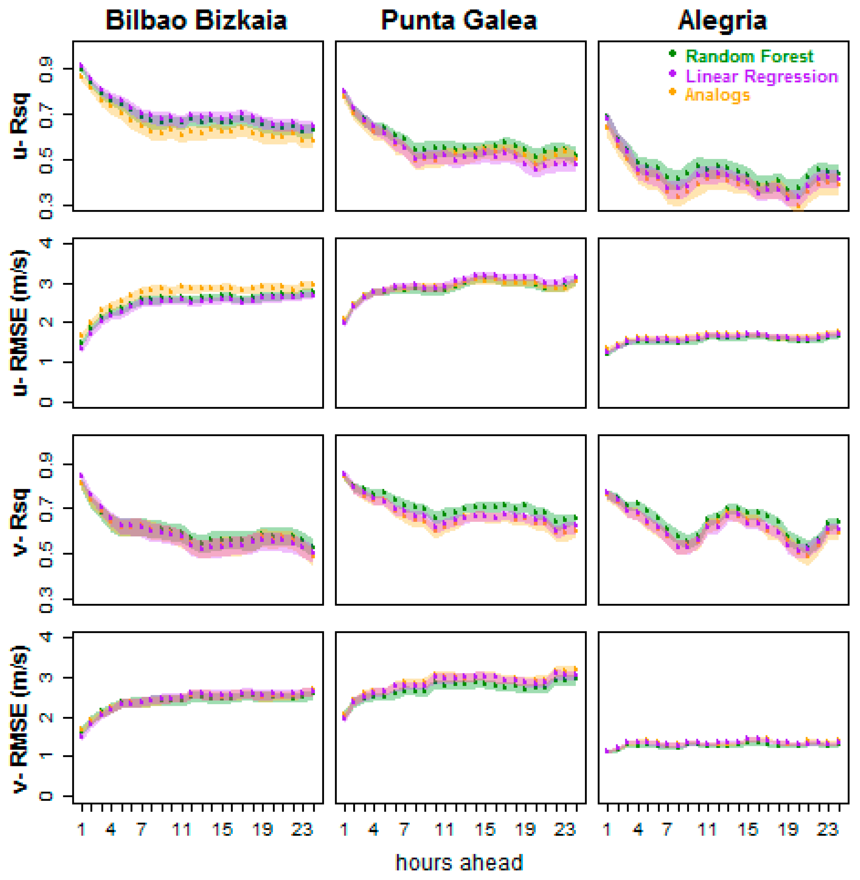
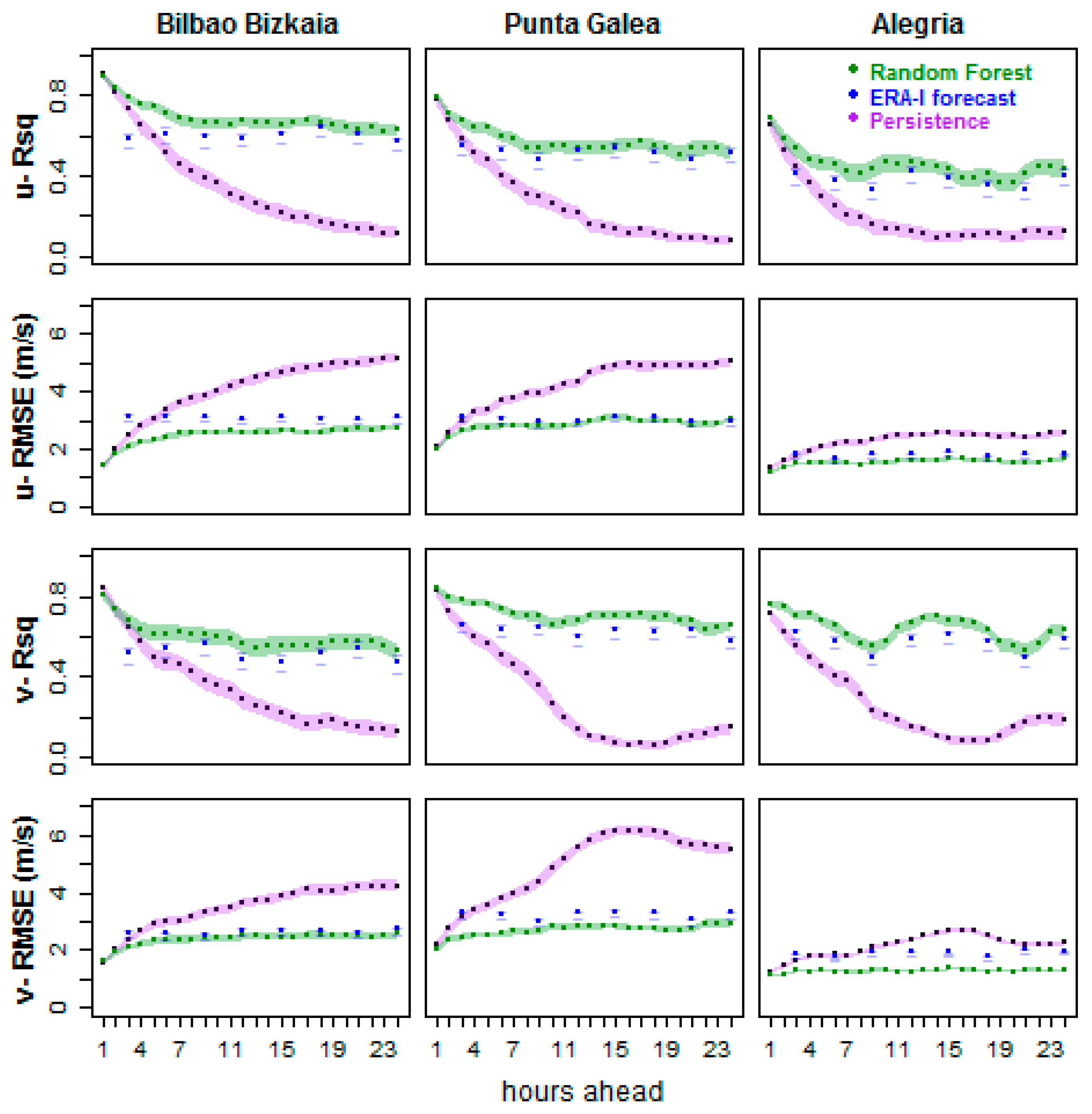
3.1.2. Model Evaluation

The next step was to compare the results of the statistical models based on RF (the best technique identified in the previous step) against persistence and ERA-Interim forecasts for the nearest grid point. The results can be seen in Figure 5 and Table 5 and Table 6 for the Bilbao Bizkaia buoy, Punta Galea, and Alegria locations. The errors of the physics-based ERA-Interim forecasts remain almost constant up to the 24 h lag forecast [74].
If u and v are jointly analyzed, the results indicate that for horizons shorter than 2–4 h, neither the RF-based models nor ERA-Interim forecasts outperform persistence. Beyond this horizon, up to 24 h in the future, for the Bilbao Bizkaia location, the RF-based models exhibit higher R2 values and lower RMSE than persistence or ERA-Interim models for u forecasts. In the case of v, both RF and ERA-Interim clearly outperform persistence. Considering that wind prediction involves a joint forecast of u and v, the results for Bilbao Bizkaia indicate that, below a forecasting horizon of 4 h, persistence is the best option, and, from 4 h to 24 h in the future, RF-based models outperform the rest, but that both are not always significantly better than ERA-Interim forecasts.
A similar pattern can be observed for the other two locations, Punta Galea and Alegria, although persistence outperformed the other techniques for a shorter forecast horizon (the first 2–4 h). For longer horizons, the ERA-Interim and RF-based models performed better, although, for v, RF models exhibited somewhat better results than ERA-Interim forecasts. For u forecasts, RF and ERA-Interim performed similarly, and a joint evaluation of wind forecasts once again indicates a slightly better overall performance of RF-based models. In all cases, it must be noted that the RMSE were lower for the different techniques and forecasting horizons for Alegria, but this was due to the lower wind speed values recorded at this location.
A seasonally stratified analysis (not shown) confirmed the abovementioned ranking, although in summer, since wind is generally weaker, the error values described by the RMSE are also smaller.

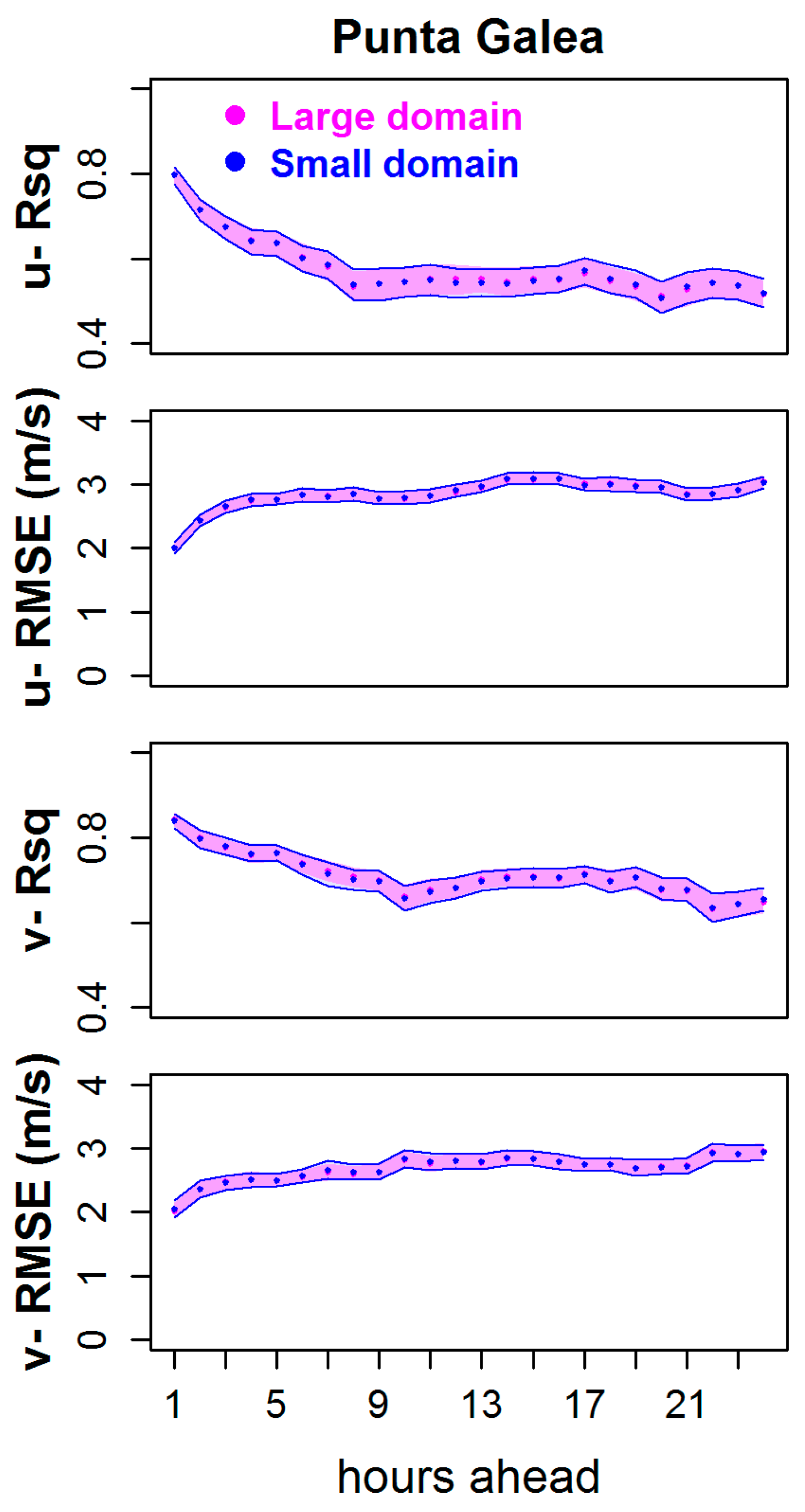
3.1.3. Sensitivity to the Domain Size

One of the input groups was the extEOF derived from the ERA-Interim values of different variables, plus local observations, as explained in Section 2.2. As mentioned above, the geographical boundaries of those variables used to calculate the extEOF were (49.50° N, 12° W) to (36° N, 7.5° E) (Figure 3). The reason that these boundaries were selected is that analysis of the variables inside this domain could allow us to capture the large-scale synoptic fields influencing the wind field at the three locations.
However, it was necessary to evaluate how the size of the selected domain could affect the results. To that end, a new set of extEOF was derived from the same variables, but defined for a smaller domain, from (45° N, 12° W) to (40° N, 0° E) (Figure 6). These new extEOFs were used to build the RF models again, and their performance was evaluated following the same method as before.
The rationale behind this testing of the domain is that the observed wind field in the Basque Country is, as is common in extratropical areas, very likely close to geostrophy. The ability of a smaller domain to provide information at this level must be checked. The use of a smaller domain would make calculations more simple, quicker, and straightforward. For this reason, a much smaller domain has also been considered.
The results of the RF-based models obtained using the two sets of extEOFs derived from the two domains can be seen in Figure 7. This figure clearly shows that the statistical indicators of performance for R2 and RMSE (95% confidence boundaries) are entirely overlapping, thus indicating a similar performance. For this reason, it can be concluded that there is negligible sensitivity of results to a domain size in the range analyzed in this paper.

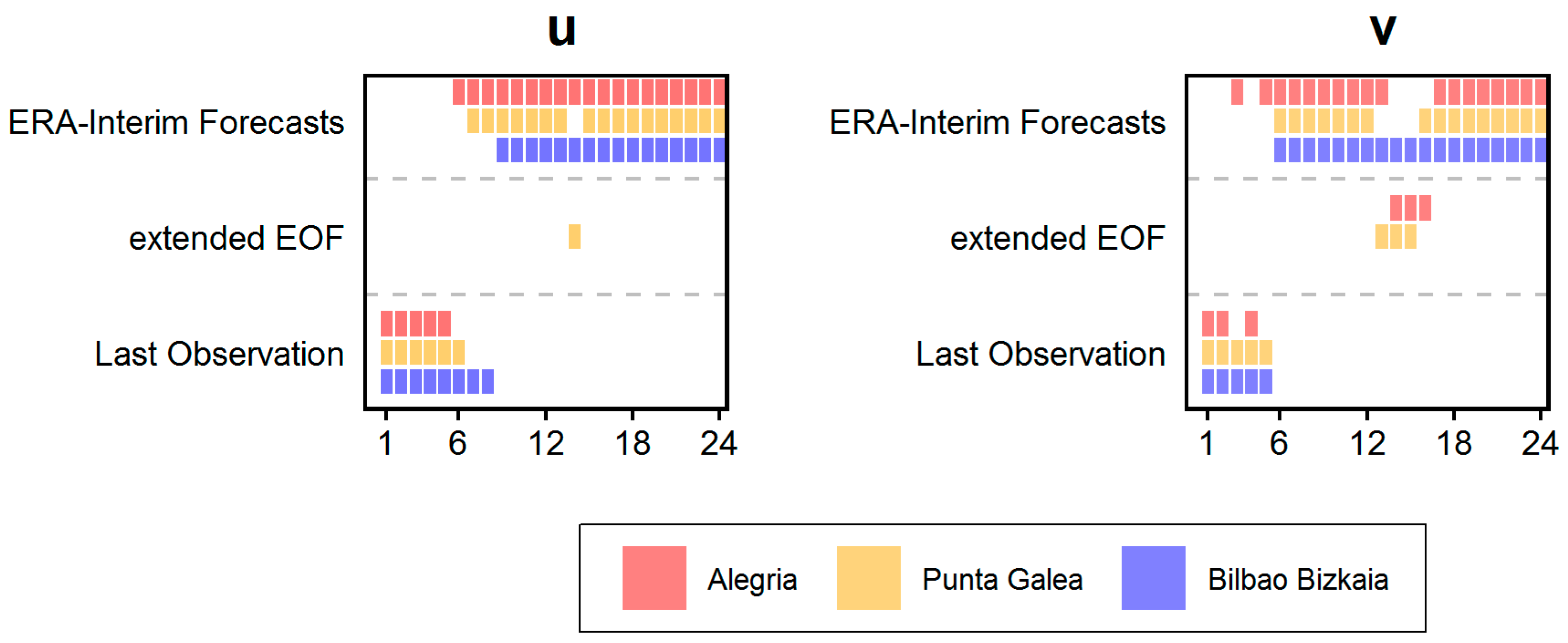
3.1.4. Identification of Relevant Inputs

The RF-based models were identified as those that, in general terms, performed best. Thus, these models were compared with the ERA-Interim and persistence forecasts. However, it should be noted that, for the three locations, the statistical models built with RF roughly identify the same three groups of inputs as being the most influential. These predictors are current local wind observation (u, v); the first, second, fourth, eighth, and ninth extEOFs; and the ERA-Interim forecasts for the nearest grid points. Figure 8 shows the most influential input for the different horizons for RF-based models.
For predictions for shorter horizons than 2–5 h, the most influential variable tends to be the current observation. This indicates that for short horizons, the system’s memory accounts for the highest fraction of overall predictability achieved by the models, which do not outperform persistence in the first 2–4 h. For medium-range predictions, persistence, ERA-Interim forecasts, and extEOFs tend to be either the most, or second most, influential inputs. Finally, for forecasting horizons longer than 7–9 h, the wind forecasts of ERA-Interim for the nearest grid points are the most influential predictors. All these conclusions are for the most important variable in each model, but if the second one (or even the third) is considered (results not shown), extEOFs become more influential.

3.2. Model Performance for Wind Gusts

Considering the results obtained under Section 3.1, the model evaluation against persistence and ERA-Interim forecasts and the identification of important inputs for the downscaling model presented in the previous subsections. The best-performing one has been used for wind gust variable.

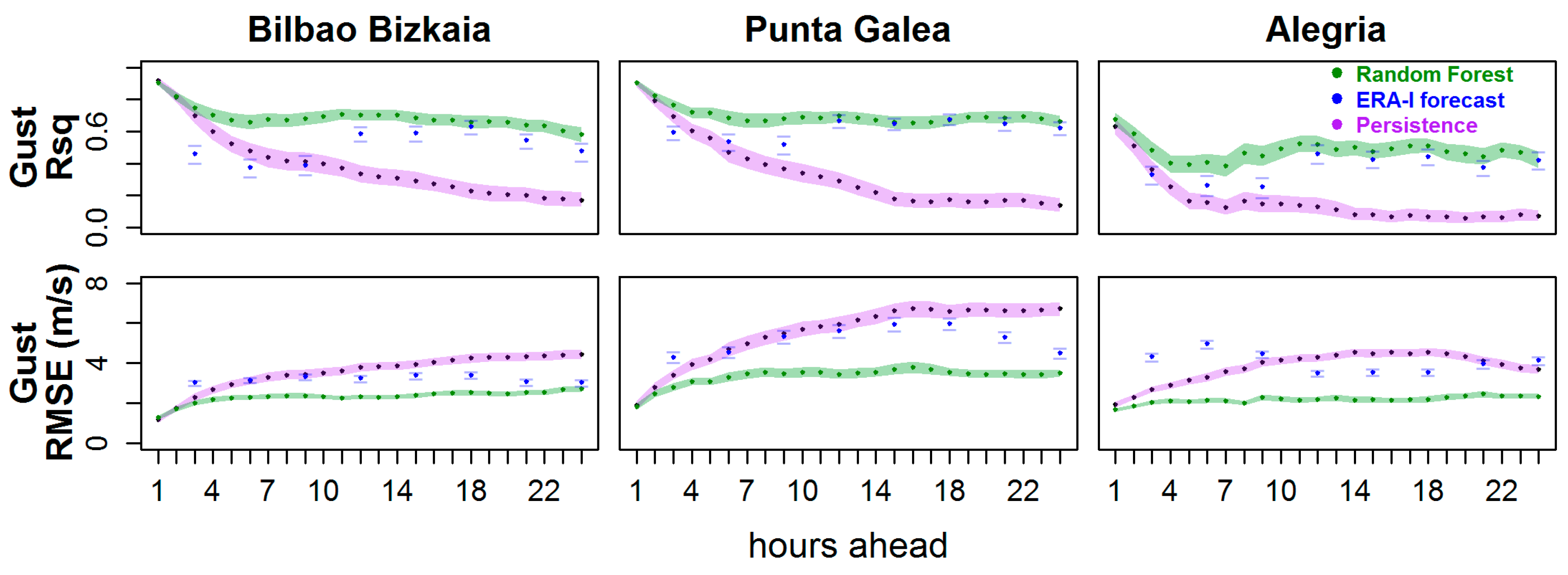
3.2.1. Model Evaluation

A similar general approach to that described above was also applied to construct the forecasting models at the same three locations, with wind gust as the target variable. The forecasting horizons were also the same (from 1 to 24 h in the future), but, since in most cases RF seemed to perform somewhat better for u and v, this was the only technique analyzed in a more detailed way. Similar predictors were also used in the models (Table 2). For this case, the inputs were:
  • All the information up to t = 0, last 3 h of observed wind gusts, and the same set of extEOFs corresponding to the initial domain and variables;
  • Instead of using the u and v values observed at time t = 0, the selected input was the maximum wind gust since previous post-processing;
  • The ERA-Interim forecasts were those corresponding to the upcoming maximum wind gusts. These forecasts involved 3 h time steps from t + 3 to t + 24 h.
Therefore, for this target variable a total of 72 RF-based models were evaluated, the results of which are shown in Figure 9 and Table 7 and Table 8. It can be seen that the best choice for modelling the first 1–2 h was persistence. From this time onwards, the results indicate that, for the three locations and all forecasting horizons, the RF-based models exhibited a significantly smaller error than either persistence or ERA-Interim forecasts. In general terms, wind gust results are better than u and v’s previously obtained results.

3.2.2. Identification of Important Inputs

The most important input for maximum wind gust forecasts over the last 3 h period is shown in Figure 10 for different lead times. The previous pattern was confirmed; in the first 4 h, the selected input was the last observation, and in the last 10 h, it was the ERA-Interim forecast for the nearest grid points. The results for the u wind component and wind gust were very similar. The horizons for persistence and ERA-Interim forecast were almost the same. They only differed in the selection of extEOFs for medium-range predictions. In the same way as previously, all these conclusions are for the most influential inputs in each model, but, if the second one (or even the third) is considered (results not shown), extEOFs gain relevance (results not shown).

4. Discussion

The approach used in this paper follows the general pattern of using forecasts provided by various types of numerical models (such as the prognostic model used in the ERA-Interim reanalysis) followed by a statistical modelling stage based on different mathematical algorithms [33]. In our case, as shown above, the models include additional candidate inputs, like extEOFs plus local observations. The comparison between the performance of analogues, linear regression, and RF indicates that RF outperforms linear regression and analogues, but not in all cases, and never overwhelmingly.
Since the persistence of wind is not null, any modelling effort must also outperform persistence (Okumus and Dinler, 2016). Persistence, and ERA-Interim forecasts (playing the role of the surrogate of an operational NWF system) represent readily available forecasting models. The performance comparison between the best statistical technique (RF) and the plain use of persistence or ERA-Interim forecasts indicates that RF outperforms the others beyond the time horizon of 1–4 h. On the other hand, persistence is always a better option than the methods tested here for up to 1–4 h into the future. Preliminary studies with a low number of cases (10 days) indicate that a modified general regression neural network could beat persistence, even for short-term horizons (below 5 h). Other studies [9,41,48], using different methods, have found that RMSE values are better than for plain persistence, even for the first hour. However, in these studies, the number of cases is not very high, and the authors do not assess the statistical significance of the performance differences. All this indicates that the specific conditions in which persistence is outperformed for very short-term forecasting horizons are yet to be fully understood, and further research in this area may be needed. In our study, for all predictands and forecasts up to 2–5 h in the future, the most influential input is the current local observation. Thus, the system’s memory plays a key role in building the prediction and explains why persistence is not beaten in these cases in the immediate short-term. Beyond this horizon, ERA-Interim forecasts are the most important predictor. The group of extEOFs (but not the same ones in all cases) also plays an important role, as the second/third most influential input, thus confirming the need to use all three general groups of inputs.
These results are in general agreement with earlier studies [7], even for the same area [18], where different statistical approaches applied to outputs from numerical models were used. Soman et al. [7] describe that, for horizons longer than 6 h, hybrid structures, such as the numerical model with post-processing, or the numerical model plus time series techniques, also exhibit better results. Santamaría-Bonfil et al. [10] and Hu et al. [50] reached the same conclusion for wind speed forecasting. More specifically, their models are based on time series with SVM and analogue methods, respectively. The authors indicate that persistence is the best model up to the 5 h horizons, signifying that they reached broadly similar conclusions to those in this study.
RF is one of the algorithms considered by Rozas-Larraondo et al. [18], but they issued forecasts only up to a 3 h lead time. In general terms, these authors combined the outputs of an NWF—GFS in this case—with METAR data as additional inputs to build a statistical model. In our study, we have extended the method to another variable (wind gust), statistical prediction techniques (analogues and linear regression), longer forecast lead times, and different data compression techniques, with the use of predictors such as extEOFs. Our results for longer lead times support the suggestion that RF-based statistical downscaling models constitute an effective tool for providing short-time wind forecasts, particularly when an NWF predictor is included in lead times longer than 3 h. Since we found that these results hold for three different locations (ocean, coast, and interior), with different wind regimes and an assessment of errors to a 95% confidence level by means of bootstrapping, we think the results are quite robust.
It must be noted that the models shown in this paper were built for three locations, representative of different areas in the region: Sea, coast, and inland. The surroundings of the three locations and the wind regimes are all very different. It must, however, be highlighted that the results show a common pattern with regard to the best statistical technique (RF) to be used, for the forecasting horizons and also for the most influential input groups. Despite this general common pattern, the particular aspects of the RF models built for the individual sites, such as the specific inputs selected at each location for each forecasting horizon (Figure 8 and Figure 10), are different. Moreover, similarly to other statistical forecasting models [8,34,39], especially for sites where complex topography is an important factor, the RF models developed here are not exchangeable, but rather site-dependent and valid only for their specific locations. Okumus and Dinler [12] also present the idea that results using similar approaches to that in this study depend on target location and data.
The distance from the locations and the nearest ERA-Interim grid points, around 14–25 km, could impact (Figure 1) the results. By applying these techniques to a higher-resolution operational model, better results from the model can be expected, because the model output would be available at a smaller distance from the wind station. As mentioned above, the wind forecasts provided by the model used in the reanalysis play an important role in building the predictions [31]. The impact of the distance between grids and points needs to be assessed with further studies, and with new reanalyses, like ERA5, since operational models are often run at much higher resolutions. In any case, if higher-resolution models were used, better inputs would also be introduced in the statistical model. Thus, it can be expected that the RF-based models’ results presented in this paper would be relatively robust to the spatial resolution of the NWF model, which provides the inputs. However, inhomogeneities in the archives derived from operational models (not the ones used in reanalyses) make this somewhat problematic when evaluating a relatively long time period (eight years), such as the period in this study.
Since meteorological services already have access to the numerical outputs from global and regional numerical models, the availability of advanced statistical methods coupled to numerical outputs, such as the one presented in this study, is important, because it allows a local wind prediction system to be developed with a lead time of several hours (1–24 h). From the perspective of meteorological agency, forecasts are very important, but especially so in emergency cases: To more accurately forecast wind speed and direction for the next 24 h when strong winds are expected, and when wind gusts are expected to surpass the threshold levels corresponding to a warning that should be issued, because, on those occasions, the wind could result in dangerous situations for the population [1,4].
Regarding other applications, it should be highlighted that the wind energy sector already uses [13] deep techniques to improve the renewable energy forecasts. Having access to wind forecasts that are as accurate as possible could help better integrate wind energy into the electric grid [6,75]. In this field, short ranges of between 10 min and 2 h are customarily used for controlling and regulating turbines. According to our results, further study is necessary at this point, because the proposed models perform more poorly than persistence for this horizon. On the other hand, electricity markets require longer prediction ranges, usually between 13 and 37 h in the future, with hourly temporal resolution. In this case, we propose that from 13 to 24 h RF forecasting should be used, while, from 24 to 37 h forecasts, an NWF model is probably the best tool (valid for ERA-Interim, at least). We hope that the method proposed in this paper can be used to optimize the position in the electricity auction market of the stakeholders in the wind energy sector, although future studies should evaluate this in detail, considering the drawbacks of higher resolution (operational models) versus longer homogeneous training length (reanalyses).

5. Conclusions

Although applied to three particular locations, the present study contains a complete method for short-term wind prediction that can easily be transferred and potentially applied elsewhere. This method involves a machine-learning technique like RF and, in addition to numerical forecasts (provided here by ERA-Interim as hindcasts) and local wind observations, it incorporates extended EOFs as additional inputs. The result is wind forecasts at hourly intervals up to 24 h in the future.
Although previously discussed in general terms, the forecasting errors of the RF-based models presented in this paper cannot be directly compared to results from previous studies. Nevertheless, it can be stated that, in absolute terms, the performance is, in general, similar to the one reported by other studies, and that errors are lower than the plain use of either persistence or direct model output from ERA-Interim. For this reason, in our study, RF-based models provide clear added value and represent a significant improvement over the use of the above-mentioned readily available forecasts for forecast horizons of 4–24 h, and sometimes 1–24 h forecasting horizons.
Below this forecasting range, the memory of the system (persistence) is the best predictor. The comparison between three different types of techniques (RF, linear regression, and analogues) evaluated in this study indicates that, in general, RF performs slightly better than the others, but not always and not for all forecasting horizons.
The results are common to the three analysed variables (u, v, and wind gust), forecasting horizons (24), and sites (three). Since the analysis covered many input cases (over 1800), many years, different locations (ocean, coastal, and inland places), and statistical techniques, we can consider this a robust outcome.
The next step in this research path, once the u and v wind components and wind gust have been analyzed, will be to apply the same method to extreme events. This requires a longer training database, due to a very low probability of this type of event, but a similar approach to that presented in this paper, based on RF and similar types of inputs, looks highly promising. ERA5 and UERRA reanalyses [54] have recently been made available with 0.3° and 1 h (ERA5) and 11 km × 11 km and 6 h (UERRA) spatial and temporal resolutions for a long time span: (1979–2018) for ERA5; and (1962–2018) for UERRA. As in the ERA-Interim model, forecasts are also available, so ERA5 or UERRA, along with RF, will be used in future studies. The prediction of extreme events and the appropriate management of this information represent important challenges for meteorological services and insurance companies. Furthermore, RF can also yield probabilistic predictions, something that is useful when different alert levels have to be launched to protect lives and properties. In this paper, different statistical models were compared for the short-term forecasting of wind and wind forecasts over the ocean, the coast, and an interior site in the Basque Country. The design of this study follows the reasoning presented in many references already discussed in the introduction to this paper [8,12,26,27,31,33]. This has also been the authors’ experience in previous papers [52,76]. It is a common result in the literature that the use of a statistical model, which is fed with data provided by a numerical weather forecast model, yields better results than the use of a statistical model alone or a numerical model alone. There are interesting new developments in the field of statistical wind forecast [45,46]. Since the regime-switch modelled in these new developments is already described by the numerical forecast that is being used to feed the postprocessing statistical model, the regime-switch is already being taken into account by the random forest model. A definition of a regime-switch technique, which blends numerical inputs to previous states of the observed wind, would be an interesting future new development.

Author Contributions

Conceptualization, S.C.-M., G.I.-B., J.S., and E.Z.; methodology, S.C.-M., G.I.-B., J.S., E.Z., and A.U.; software, S.C.-M. and G.I.-B.; validation, S.C.-M. and G.I.-B.; writing—original draft preparation, S.C.-M., G.I.-B., and J.S.; writing—review and editing, G.I.-B., J.S., E.Z., and A.U.; visualization, S.C.-M.; supervision, G.I.-B., J.S., E.Z., and A.U.; funding acquisition, G.I.-B. and J.S. All authors have read and agreed to the published version of the manuscript.

Funding

This work was supported by the Spanish Government, MINECO project CGL2016-76561-R (MINECO/EU ERDF), and the University of the Basque Country (project GIU17/02).

Acknowledgments

The ECMWF ERA-Interim data used in this study are freely available and were downloaded from the ECMWF-MARS Data Server at no cost. The authors would like to express their gratitude to Puertos del Estado for kindly providing the data for this study. More particularly, the authors want to thank the Emergencies and Meteorology Directorate (Basque Regional Government) for public provision of data and operational service financial support. Most of the calculations and plots were carried out within the framework of R [77] and GMT [78].

Conflicts of Interest

The authors declare no conflict of interest.

References

  1. Freebairn, J.W.; Zillman, J.W. Economic benefits of meteorological services. Meteorol. Appl. 2002, 9, 33–44. [Google Scholar] [CrossRef] [Green Version]
  2. Spanish Deparment of Economy Industry and Competitiveness. The Spanish Extraordinary Risk Coverage System; Spanish Deparment of Economy Industry and Competitiveness: Madrid, Spian, 2016; pp. 1987–2015. [Google Scholar]
  3. Liberato, M.L.R.; Pinto, J.G.; Trigo, I.F.; Trigo, R.M. Klaus-An exceptional winter storm over northern Iberia and southern France. Weather 2011, 66, 330–334. [Google Scholar] [CrossRef] [Green Version]
  4. Solari, G.; Repetto, M.P.; Burlando, M.; de Gaetano, P.; Pizzo, M.; Tizzi, M.; Parodi, M. The wind forecast for safety management of port areas. J. Wind Eng. Ind. Aerodyn. 2012, 104, 266–277. [Google Scholar] [CrossRef]
  5. Ibarra-Berastegi, G.; Elias, A.; Barona, A.; Saenz, J.; Ezcurra, A.; Diaz de Argandoña, J. From diagnosis to prognosis for forecasting air pollution using neural networks: Air pollution monitoring in Bilbao. Environ. Model. Softw. 2008, 23, 622–637. [Google Scholar] [CrossRef]
  6. Pinson, P. Wind Energy: Forecasting Challenges for Its Operational Management. Stat. Sci. 2013, 28, 564–585. [Google Scholar] [CrossRef] [Green Version]
  7. Soman, S.S.; Zareipour, H.; Malik, O.; Mandal, P. A review of wind power and wind speed forecasting methods with different time horizons. In Proceedings of the North American Power Symposium 2010, Arlington, TX, USA, 26–28 September 2010. [Google Scholar] [CrossRef]
  8. Cassola, F.; Burlando, M. Wind speed and wind energy forecast through Kalman filtering of Numerical Weather Prediction model output. Appl. Energy 2012, 99, 154–166. [Google Scholar] [CrossRef]
  9. Barbounis, T.G.; Theocharis, J.B.Ã. Locally recurrent neural networks for long-term wind speed and power prediction. Neurocomputing 2006, 69, 466–496. [Google Scholar] [CrossRef]
  10. Santamaría-Bonfil, G.; Reyes-Ballesteros, A.; Gershenson, C. Wind speed forecasting for wind farms: A method based on support vector regression. Renew. Energy 2016, 85, 790–809. [Google Scholar] [CrossRef]
  11. Feng, C.; Cui, M.; Hodge, B.M.; Zhang, J. A data-driven multi-model methodology with deep feature selection for short-term wind forecasting. Appl. Energy 2017, 190, 1245–1257. [Google Scholar] [CrossRef] [Green Version]
  12. Okumus, I.; Dinler, A. Current status of wind energy forecasting and a hybrid method for hourly predictions. Energy Convers. Manag. 2016, 123, 362–371. [Google Scholar] [CrossRef]
  13. Wang, H.; Lei, Z.; Zhang, X.; Zhou, B.; Peng, J. A review of deep learning for renewable energy forecasting. Energy Convers. Manag. 2019, 198, 111799. [Google Scholar] [CrossRef]
  14. Cheney, N.P.; Gould, J.S.; Catchpole, W.R. The Influence Of Fuel, Weather And Fire Shape Variables On Fire-Spread In Grasslands. Int. J. Wildl. Fire 1993, 3, 31–44. [Google Scholar] [CrossRef]
  15. Del Prete, R.; Pezzoli, A.; Pezzoli, G. Current methods for meteorological and marine forecasting for the assistance of navigation and shipping operations. J. Navig. 1999, 52, 104–118. [Google Scholar] [CrossRef]
  16. Tagliaferri, F.; Viola, I.M.; Flay, R.G.J. Wind direction forecasting with artificial neural networks and support vector machines. Ocean Eng. 2015, 97, 65–73. [Google Scholar] [CrossRef] [Green Version]
  17. Traveria, M.; Escribano, A.; Palomo, P. Statistical wind forecast for Reus airport. Meteorol. Appl. 2010, 17, 485–495. [Google Scholar] [CrossRef]
  18. Rozas-Larraondo, P.; Inza, I.; Lozano, J.A. A Method for Wind Speed Forecasting in Airports Based on Nonparametric Regression. Weather Forecast. 2014, 29, 1332–1342. [Google Scholar] [CrossRef]
  19. Lewis, J.M.; Lakshmivarahan, S.; Dhall, S. Dynamic Data Assimilation; Cambridge University Press: Cambridge, UK, 2009. [Google Scholar]
  20. Cushman-Roisin, B.; Beckers, J.-M. Introduction to Geophysical Fluid Dynamics - Physical and Numerical Aspects. Int. Geophys. 2011, 101, 701–724. [Google Scholar]
  21. Dee, D.P.; Uppala, S.M.; Simmons, A.J.; Berrisford, P.; Poli, P.; Kobayashi, S.; Andrae, U.; Balmaseda, M.A.; Balsamo, G.; Bauer, P.; et al. The ERA-Interim reanalysis: Configuration and performance of the data assimilation system. Q. J. R. Meteorol. Soc. 2011, 137, 553–597. [Google Scholar] [CrossRef]
  22. Kalnay, E.; Kanamitsu, M.; Kistler, R.; Collins, W.; Deaven, D.; Gandin, L.; Iredell, M.; Saha, S.; White, G.; Woollen, J.; et al. The NCEP/NCAR 40-year reanalysis project. Bull. Am. Meteorol. Soc. 1996, 77, 437–471. [Google Scholar] [CrossRef] [Green Version]
  23. Skamarock, W.C.; Klemp, J.B.; Dudhi, J.; Gill, D.O.; Barker, D.M.; Duda, M.G.; Huang, X.-Y.; Wang, W.; Powers, J.G. A Description of the Advanced Research WRF Version 3. NCAR Tech. Note NCAR/TN-475+STR; University Corporation for Atmospheric Research: Boulder, CO, USA, 2008; p. 113. [Google Scholar]
  24. Pielke, R.A.; Cotton, W.R.; Walko, R.L.; Tremback, C.J.; Lyons, W.A.; Grasso, L.D.; Nicholls, M.E.; Moran, M.D.; Wesley, D.A.; Lee, T.J.; et al. A comprehensive meteorological modeling system-RAMS. Meteorol. Atmos. Phys. 1992, 49, 69–91. [Google Scholar] [CrossRef]
  25. Unden, P.; Rontu, L.; Jarvinen, H.; Lynch, P.; Calvo, J.; Cats, G.; Cuxart, J.; Eerola, K.; Fortelius, C.; Garcia-moya, J.A.; et al. HIRLAM-5 Scientific Documentation. 2002. Available online: http://citeseerx.ist.psu.edu/viewdoc/summary?doi=10.1.1.6.3794 (accessed on 28 November 2019).
  26. Valero, F.; Pascual, A.; Martín, M.L. An approach for the forecasting of wind strength tailored to routine observational daily wind gust data. Atmos. Res. 2014, 137, 58–65. [Google Scholar] [CrossRef]
  27. Pascual, A.; Valero, F.; Martín, M.L.; Morata, A.; Luna, M.Y. Probabilistic and deterministic results of the ANPAF analog model for Spanish wind field estimations. Atmos. Res. 2012, 108, 39–56. [Google Scholar] [CrossRef]
  28. Environmental Modeling Center. The GFS Atmospheric Model, Note 442; Environmental Modeling Center: College Park, MA, USA, 2003.
  29. Janjic, Z.; Gall, R.; Pyle, M.E. Scientific Doucmentation for NMM Solver. 2010. Available online: https://opensky.ucar.edu/islandora/object/technotes%3A490 (accessed on 28 November 2019).
  30. Benjamin, S.G.; Grell, G.A.; Brown, J.M.; Smirnova, T.G.; Bleck, R. Mesoscale Weather Prediction with the RUC Hybrid Isentropic–Terrain-Following Coordinate Model. Mon. Weather. Rev. 2004, 132, 473–494. [Google Scholar] [CrossRef]
  31. Nagarajan, B.; Delle Monache, L.; Hacker, J.P.; Rife, D.L.; Searight, K.; Knievel, J.C.; Nipen, T.N. An Evaluation of Analog-Based Postprocessing Methods across Several Variables and Forecast Models. Weather Forecast. 2015, 30, 1623–1643. [Google Scholar] [CrossRef]
  32. Buzzi, A.; Fantini, M.; Malguzzi, P.; Nerozzi, F. Validation of a limited area model in cases of mediterranean cyclogenesis: Surface fields and precipitation scores. Meteorol. Atmos. Phys. 1994, 53, 137–153. [Google Scholar] [CrossRef]
  33. Zhao, W.; Wei, Y.M.; Su, Z. One day ahead wind speed forecasting: A resampling-based approach. Appl. Energy 2016, 178, 886–901. [Google Scholar] [CrossRef]
  34. Manor, A.; Berkovic, S. Bayesian Inference aided analog downscaling for near-surface winds in complex terrain. Atmos. Res. 2015, 164–165, 27–36. [Google Scholar] [CrossRef]
  35. Patlakas, P.; Drakaki, E.; Galanis, G.; Drakaki, E. Wind gust estimation by combining a numerical weather prediction model and statistical post-processing. Energy Procedia 2017, 125, 190–198. [Google Scholar] [CrossRef]
  36. Spyrou, C.; Mitsakou, C.; Kallos, G.; Louka, P.; Vlastou, G. An improved limited area model for describing the dust cycle in the atmosphere. J. Geophys. Res. Atmos. 2010, 115, 1–19. [Google Scholar] [CrossRef]
  37. Zjavka, L. Wind speed forecast correction models using polynomial neural networks. Renew. Energy 2015, 83, 998–1006. [Google Scholar] [CrossRef]
  38. Bouttier, F. The Météo-France NWP System: Description, Recent Changes and Plans. 2010. Available online: http://www.umr-cnrm.fr/gmap/nwp/nwpreport.pdf (accessed on 28 November 2019).
  39. Fernández-Ferrero, A.; Sáenz, J.; Ibarra-Berastegi, G.; Fernández, J. Evaluation of statistical downscaling in short range precipitation forecasting. Atmos. Res. 2009, 94, 448–461. [Google Scholar] [CrossRef]
  40. Raible, C.C.; Bischof, G.; Fraedrich, K.; Kirk, E. Statistical Single-Station Short-Term Forecasting of Temperature and Probability of Precipitation: Area Interpolation and NWP Combination. Weather Forecast. 1999, 14, 203–214. [Google Scholar] [CrossRef]
  41. Torres, J.L.; García, A.; De Blas, M.; De Francisco, A. Forecast of hourly average wind speed with ARMA models in Navarre (Spain). Sol. Energy 2005, 79, 65–77. [Google Scholar] [CrossRef]
  42. Müller, M.D. Effects of model resolution and statistical postprocessing on shelter temperature and wind forecasts. J. Appl. Meteorol. Climatol. 2011, 50, 1627–1636. [Google Scholar] [CrossRef] [Green Version]
  43. Kulkarni, M.A.; Patil, S.; Rama, G.V.; Sen, P.N. Wind speed prediction using statistical regression and neutral network. J. Earth Syst. Sci. 2008, 117, 457–463. [Google Scholar] [CrossRef] [Green Version]
  44. Li, G.; Shi, J. On comparing three artificial neural networks for wind speed forecasting. Appl. Energy 2010, 87, 2313–2320. [Google Scholar] [CrossRef]
  45. Ezzat, A.A.; Jun, M.; Ding, Y. Spatio-temporal short-term wind forecast: A calibrated regime-switching method By Ahmed Aziz Ezzat, Mikyoung Jun and Yu Ding Texas A&M University. Ann. Appl. Stat. 2019, 13, 1484–1510. [Google Scholar]
  46. Ding, Y. Data Science for Wind Energy; Chapman & Hall/CRC: Boca Raton, FL, USA, 2019; ISBN 9781138590526. [Google Scholar]
  47. Liu, H.; Tian, H.Q.; Li, Y.F. Comparison of two new ARIMA-ANN and ARIMA-Kalman hybrid methods for wind speed prediction. Appl. Energy 2012, 98, 415–424. [Google Scholar] [CrossRef]
  48. Ahmed, A.; Khalid, M.; Ahmed, A.; Khalid, M. Multi-step Ahead Wind Forecasting Using Nonlinear Autoregressive Neural Networks. Energy Procedia 2017, 134, 192–204. [Google Scholar] [CrossRef]
  49. Zorita, E.; von Storch, H. The analog method as a simple statistical downscaling technique:comparison with more complicated methods. J. Clim. 1999, 12, 2474–2489. [Google Scholar] [CrossRef]
  50. Hu, Q.; Su, P.; Yu, D.; Liu, J. Pattern-Based Wind Speed Prediction Based on Generalized Principal Component Analysis. Sustain. Energy IEEE Trans. 2014, 5, 866–874. [Google Scholar] [CrossRef]
  51. do Camelo, H.N.; Lucio, P.S.; Junior, J.B.V.L.; von Glehn dos Santos, D.; de Carvalho, P.C.M. Innovative hybrid modeling ofwind speed prediction involving time-series models and artificial neural networks. Atmosphere 2018, 9, 77. [Google Scholar]
  52. Ibarra-Berastegi, G.; Saénz, J.; Esnaola, G.; Ezcurra, A.; Ulazia, A. Short-term forecasting of the wave energy flux: Analogues, random forests, and physics-based models. Ocean Eng. 2015, 104, 530–539. [Google Scholar] [CrossRef]
  53. Puertos del Estado. Available online: http://www.puertos.es/es-es (accessed on 3 March 2019).
  54. ECMWF | Public Datasets. Available online: https://apps.ecmwf.int/datasets/ (accessed on 3 March 2019).
  55. Ibarra-Berastegi, G.; Saénz, J.; Ezcurra, A.; Elías, A.; Diaz Argandoña, J.; Errasti, I. Downscaling of surface moisture flux and precipitation in the Ebro Valley (Spain) using analogues and analogues followed by random forests and multiple linear regression. Hydrol. Earth Syst. Sci. 2011, 15, 1895–1907. [Google Scholar] [CrossRef]
  56. Hannachi, A.; Jolliffe, I.T.; Stephenson, D.B. Review Empirical orthogonal functions and related techniques in atmospheric science: A review. Int. J. Climatol. 2007, 27, 1119–1152. [Google Scholar] [CrossRef]
  57. Weare, B.C.; Nasstrom, J.S. Examples of Extended Empirical Orthogonal Function Analyses. Mon. Weather. Rev. 1982, 110, 481–485. [Google Scholar] [CrossRef]
  58. Fukutomi, Y.; Yasunari, T. Structure and characteristics of submonthly-scale waves along the Indian Ocean ITCZ. Clim. Dyn. 2013, 40, 1819–1839. [Google Scholar] [CrossRef] [Green Version]
  59. Tangang, F.T.; Tang, B.; Monahan, A.H.; Hsieh, W.W. Forecasting ENSO events: A neural network-extended EOF approach. J. Clim. 1998, 11, 29–41. [Google Scholar] [CrossRef]
  60. Matulla, C.; Zang, X.; Wang, X.L.; Wang, J.; Zorita, E.; Wagner, S.; von Storch, H. Influence of similarity measures on the performance of the analog method for downscaling daily precipitation. Clim. Dyn. 2008, 30, 133–144. [Google Scholar] [CrossRef]
  61. Breiman, L. Random Forests. Mach. Learn. 2001, 45, 5–32. [Google Scholar] [CrossRef] [Green Version]
  62. Quinlan, J.R. Induction of decision trees. Mach. Learn. 1986, 1, 81–106. [Google Scholar] [CrossRef] [Green Version]
  63. Grömping, U. Variable importance assessment in regression: Linear regression versus random forest. Am. Stat. 2009, 63, 308–319. [Google Scholar] [CrossRef]
  64. Liaw, A.; Wiener, M. Classification and regression by randomForest. R News 2:18-22. Forest 2001, 23, 18–22. [Google Scholar]
  65. Siroky, D.S. Navigating random forests and related advances in algorithmic modeling. Stat. Surv. 2009, 3, 147–163. [Google Scholar] [CrossRef] [Green Version]
  66. Akaike, H. Factor analysis and AIC. Psychometrik 1987, 52, 317–332. [Google Scholar] [CrossRef]
  67. Weisberg, S. Applied Linear Regression; Wiley: Hoboken, NJ, USA, 2005. [Google Scholar]
  68. Eccel, E.; Ghielmi, L.; Granitto, P.; Barbiero, R.; Grazzini, F.; Cesari, D. Prediction of minimum temperatures in an alpine region by linear and non-linear post-processing of meteorological models. Nonlinear Process. Geophys. 2007, 14, 211–222. [Google Scholar] [CrossRef] [Green Version]
  69. Lahouar, A.; Ben Hadj Slama, J. Hour-ahead wind power forecast based on random forests. Renew. Energy J. 2017, 109, 529–541. [Google Scholar] [CrossRef]
  70. Serras, P.; Ibarra-Berastegi, G.; Sáenz, J.; Ulazia, A. Combining random forests and physics-based models to forecast the electricity generated by ocean waves: A case study of the Mutriku wave farm. Ocean Eng. 2019, 189, 106314. [Google Scholar] [CrossRef]
  71. Hastie, T.; Tibsharani, R.; Friedman, J. The Elements of Statistical Learning; Springer: Berlin, Germany, 2001; Volume 27, ISBN 9780387848570. [Google Scholar]
  72. Stanski, H.R.; Wilson, L.J.; Burrows, W.R. Survey of Common Verfication Methods in Meteorology. Atmos. Res. 1989, 9–42. [Google Scholar]
  73. Efron, B. Bootstrap Methods: Another Look at the Jackknife. Ann. Stat. 1979, 7, 1–26. [Google Scholar] [CrossRef]
  74. Haiden, T.; Janousek, M.; Bidlot, J.; Ferranti, L.; Prates, F.; Vitart, F.; Richardson, D.; Bauer, P. Evaluation of ECMWF Forecasts, Including the 2016 Resolution Upgrade; ECMWF: Shinfield, UK, 2016. [Google Scholar] [CrossRef]
  75. Kariniotakis, G.; Halliday, J.; Brownsword, R.; Marti, I.; Palomares, A.M.; Cruz, I.; Madsen, H.; Nielsen, T.S.; Nielsen, H.A.; Focken, U.; et al. Next Generation Short-Term Forecasting of Wind Power―Overview of the ANEMOS Project. Eur. Wind Energy Conf. EWEC. 2006. Available online: http://www.ewec2006proceedings.info/all (accessed on 28 November 2019).
  76. Ibarra-berastegi, G.; Sáenz, J.; Ulazia, A.; Serras, P.; Esnaola, G. Electricity production, capacity factor, and plant efficiency index at the Mutriku wave farm (2014–2016). Ocean Eng. 2018, 147, 20–29. [Google Scholar] [CrossRef] [Green Version]
  77. R Core Team. R: A Language and Environment for Statistical Computing; R Found Stat. Comput.: Vienna, Austria, 2018. Available online: http://softlibre.unizar.es/manuales/aplicaciones/r/fullrefman.pdf (accessed on 28 November 2019).
  78. Wessel, P.; Smith, W.H.F.; Scharroo, R.; Luis, J.; Wobbe, F. The Generic Mapping Tools (GMT) version 5 GMT 5: A major new release of the Generic Mapping Tools. Generic Mapp. Tools (GMT) 2011, 7, 2–5. [Google Scholar]
Figure 1. Locations of interest, Bilbao Bizkaia buoy (blue circle), Punta Galea station (orange circle), Alegria station (red circle). Distances in km to the nearest ERA-Interim node (magenta star) and from the coast to the Bizkaia buoy.
Atmosphere 11 00045 g001
Figure 2. Wind roses corresponding to the period (2007–2014).
Atmosphere 11 00045 g002
Figure 3. ERA-Interim domain used for downloading analysis data.
Atmosphere 11 00045 g003
Figure 4. R2 and root mean square error (RMSE) verification indices of u and v wind components for the coming 24 h, for three locations, and three statistical methods.
Atmosphere 11 00045 g004
Figure 5. R2 and RMSE verification indices of u and v wind components for the coming 24 h, for three locations (Bilbao Bizkaia, Punta Galea, and Alegria), and comparing three methods in the test period.
Atmosphere 11 00045 g005
Figure 6. ERA-Interim domains used for downloading analyses.
Atmosphere 11 00045 g006
Figure 7. R2 and RMSE verification indices for the u and v wind components for the coming 24 h at Punta Galea, using the RF method to compare the results in two different domains.
Atmosphere 11 00045 g007
Figure 8. Most important input (last observation, extEOF, or ERA-I Forecast) of u and v wind components for the coming 24 h, at three locations using the RF method.
Atmosphere 11 00045 g008
Figure 9. R2 and RMSE verification indices for wind gust components over the coming 24 h, at three locations, and comparing three methods for the test period.
Atmosphere 11 00045 g009
Figure 10. Most important input (last observation, extended empirical orthogonal functions (extEOFs), or ERA-Interim forecast) for the wind gust for the next 24 h, at three locations (Bilbao Bizkaia, Punta Galea, and Alegria), and using the RF method.
Atmosphere 11 00045 g010
Table 1. Number of cases in each location and period.
DataTrainTest
Bilbao Bizkaia Buoy379218961896
Punta Galea Station446122312230
Alegria Station408420422042
Table 2. Summary description of the statistical model raw inputs Input.
NameVariables SourceTime
Last obsu, v, wind gust Observationst h
ERA-I Forecastu10, v10, wind gustERA-I forecastt + 3, t + 6, … t + 24 h
ExtEOFMsl, u10, v10, T2 (domain) u, v, wind gustERA-I analisis Observationst, t − 6, t − 12, t − 18 h
Table 3. R2 verification index of u and v wind components for the steps 1, 6, 12, 18, and 24 h, for three locations (Bilbao Bizkaia, Punta Galea, and Alegria), and three statistical methods (random forest, analogs, and linear regression). The best verification values are typed using bold font.
1 h6 h12 h18 h24 h
uBBRF0.89–0.910.69–0.740.65–0.70.64–0.70.6–0.65
AN0.85–0.880.64–0.70.59–0.650.58–0.650.55–0.61
LR0.9–0.920.7–0.750.67–0.720.65–0.710.62–0.67
PGRF0.78–0.820.57–0.630.51–0.580.52–0.590.49–0.55
AN0.75–0.790.53–0.590.48–0.550.49–0.560.47–0.54
LR0.78–0.820.54–0.610.46–0.530.47–0.540.45–0.51
AlRF0.65–0.710.42–0.50.42–0.510.37–0.450.39–0.48
AN0.6–0.670.37–0.450.37–0.460.33–0.420.34–0.43
LR0.64–0.710.38–0.460.39–0.470.33–0.40.37–0.46
vBBRF0.78–0.830.57–0.650.52–0.60.51–0.60.48–0.57
AN0.78–0.830.58–0.650.5–0.580.51–0.590.45–0.53
LR0.82–0.860.59–0.660.49–0.570.51–0.590.46–0.54
PGRF0.82–0.860.71–0.760.66–0.710.67–0.720.63–0.68
AN0.82–0.860.66–0.710.61–0.660.62–0.670.57–0.63
LR0.83–0.870.67–0.720.62–0.670.64–0.680.59–0.65
AlRF0.75–0.790.62–0.680.64–0.690.61–0.660.61–0.67
AN0.74–0.780.57–0.630.61–0.660.56–0.620.56–0.62
LR0.75–0.790.58–0.640.59–0.640.56–0.620.58–0.63
Table 4. RMSE verification index of u and v wind components for the steps 1, 6, 12, 18, and 24 h, for three locations (Bilbao Bizkaia, Punta Galea, and Alegria), and three statistical methods (random forest, analogs, and linear regression). Lowest values of RMSE are written using bold font.
1 h6 h12 h18 h24 h
uBBRF1.41–1.552.33–2.552.46–2.662.49–2.732.65–2.84
AN1.58–1.752.53–2.782.72–2.942.73–2.962.83–3.04
LR1.24–1.422.27–2.492.4–2.582.43–2.652.57–2.77
PGRF1.92–2.092.74–2.942.81–32.9–3.122.94–3.13
AN2–2.182.79–2.982.85–3.052.91–3.12.94–3.14
LR1.89–2.082.81–32.94–3.133.04–3.233.03–3.22
AlRF1.15–1.271.43–1.581.54–1.691.5–1.651.59–1.74
AN1.26–1.391.5–1.661.63–1.761.53–1.691.67–1.82
LR1.17–1.291.48–1.641.61–1.731.54–1.71.63–1.77
vBBRF1.53–1.742.24–2.52.36–2.612.4–2.692.45–2.69
AN1.56–1.732.23–2.472.43–2.672.43–2.72.55–2.79
LR1.38–1.582.21–2.442.45–2.692.45–2.712.52–2.75
PGRF1.92–2.182.47–2.682.7–2.922.66–2.862.83–3.06
AN1.91–2.142.67–2.92.9–3.142.84–3.073.06–3.3
LR1.84–2.072.65–2.852.86–3.072.8–3.012.95–3.17
AlRF1.07–1.161.2–1.31.21–1.31.21–1.311.23–1.34
AN1.08–1.171.27–1.391.27–1.371.28–1.391.31–1.43
LR1.07–1.151.27–1.371.29–1.381.28–1.381.3–1.39
Table 5. R2 index (95% confidence interval) of u and v wind components for the steps 1, 6, 12, 18, and 24 h, for three locations (Bilbao Bizkaia, Punta Galea, and Alegria), and RF, ERA-Interim forecasts, and persistence models. Highest values of R2 are highlighted by means of bold font.
1 h6 h12 h18 h24 h
uBBRF0.89–0.910.69–0.740.65–0.70.64–0.70.6–0.65
ERA-I F 0.57–0.650.56–0.620.61–0.670.54–0.6
Pers0.89–0.920.48–0.560.25–0.330.14–0.210.09–0.14
PGRF0.78–0.820.57–0.630.51–0.580.52–0.590.49–0.55
ERA-I F 0.49–0.560.49–0.550.48–0.550.48–0.55
Pers0.75–0.80.35–0.440.18–0.250.09–0.150.06–0.11
AlRF0.65–0.710.42–0.50.42–0.510.37–0.450.39–0.48
ERA-I F 0.34–0.420.38–0.460.31–0.390.36–0.44
Pers0.62–0.690.2–0.290.09–0.160.08–0.150.08–0.16
vBBRF0.78–0.830.57–0.650.52–0.60.51–0.60.48–0.57
ERA-I F 0.5–0.580.45–0.530.48–0.560.43–0.51
Pers0.81–0.860.43–0.520.25–0.330.14–0.220.09–0.16
PGRF0.82–0.860.71–0.760.66–0.710.67–0.720.63–0.68
ERA-I F 0.61–0.660.57–0.630.6–0.650.55–0.61
Pers0.8–0.850.46–0.540.11–0.170.04–0.080.12–0.18
AlRF0.75–0.790.62–0.680.64–0.690.61–0.660.61–0.67
ERA-I F 0.55–0.610.56–0.620.55–0.60.56–0.61
Pers0.68–0.740.36–0.440.12–0.180.06–0.110.15–0.22
Table 6. RMSE index (95% confidence interval) of u and v wind components for the steps 1, 6, 12, 18, and 24 h, for three locations (Bilbao Bizkaia, Punta Galea, and Alegria), and RF, ERA-Interim forecasts, and persistence models. Lowest values of RMSE are highlighted by means of bold font.
1 h6 h12 h18 h24 h
uBBRF1.41–1.552.33–2.552.46–2.662.49–2.732.65–2.84
ERA-I F 3.05–3.272.97–3.172.97–3.183–3.21
Pers1.31–1.513.21–3.564.15–4.54.7–5.075–5.37
PGRF1.92–2.092.74–2.942.81–32.9–3.122.94–3.13
ERA-I F 3–3.182.87–3.053.02–3.22.92–3.11
Pers1.95–2.23.51–3.844.21–4.524.74–5.094.9–5.25
AlRF1.15–1.271.43–1.581.54–1.691.5–1.651.59–1.74
ERA-I F 1.63–1.781.77–1.891.69–1.851.82–1.95
Pers1.28–1.442.06–2.292.42–2.642.37–2.582.42–2.65
vBBRF1.53–1.742.24–2.52.36–2.612.4–2.692.45–2.69
ERA-I F 2.46–2.692.58–2.832.55–2.792.62–2.86
Pers1.44–1.662.82–3.153.45–3.783.9–4.254.05–4.44
PGRF1.92–2.182.47–2.682.7–2.922.66–2.862.83–3.06
ERA-I F 3.15–3.373.17–3.43.17–3.383.19–3.42
Pers2–2.313.63–3.985.39–5.765.92–6.315.32–5.74
AlRF1.07–1.161.2–1.31.21–1.31.21–1.311.23–1.34
ERA-I F 1.69–1.811.86–1.991.72–1.841.91–2.05
Pers1.2–1.321.76–1.922.31–2.452.45–2.592.2–2.36
Table 7. R2 index (95% confidence interval) of wind gust for the steps 1, 6, 12, 18, and 24 h, for three locations (Bilbao Bizkaia, Punta Galea, and Alegria), and RF, ERA-Interim forecasts, and persistence models. The results corresponding to the best model are highlighted using bold font.
1 h6 h12 h18 h24 h
GustBBRF0.9–0.930.67–0.720.64–0.690.61–0.670.58–0.64
ERA-I F 0.38–0.460.45–0.530.39–0.470.43–0.51
Pers0.9–0.930.49–0.570.31–0.40.19–0.260.16–0.22
PGRF0.9–0.920.68–0.730.65–0.710.62–0.680.63–0.69
ERA-I F 0.5–0.570.58–0.640.49–0.550.56–0.62
Pers0.9–0.930.45–0.530.24–0.310.13–0.20.12–0.18
AlRF0.73–0.780.51–0.580.54–0.610.47–0.530.5–0.57
ERA-I F 0.37–0.450.48–0.550.36–0.440.47–0.54
Pers0.69–0.750.28–0.360.02–0.060–0.030.12–0.19
Table 8. RMSE index (95% confidence interval) of wind gust for the steps 1, 6, 12, 18, and 24 h, for three locations (Bilbao Bizkaia, Punta Galea, and Alegria), and RF, ERA-Interim forecasts, and persistence models. Lowest RMSE values are highlighted by using bold font.
1 h6 h12 h18 h24 h
GustBBRF1.14–1.282.19–2.352.34–2.532.4–2.572.55–2.74
ERA-I F 3.22–3.422.98–3.23.18–3.383.05–3.27
Pers1.09–1.272.88–3.153.57–3.864.02–4.344.26–4.59
PGRF1.67–1.923.11–3.423.31–3.633.42–3.723.44–3.79
ERA-I F 5.16–5.534.91–5.325.15–5.554.86–5.29
Pers1.67–1.964.49–4.945.72–6.26.36–6.896.48–7.03
AlRF1.59–1.771.98–2.172.07–2.272.07–2.32.17–2.36
ERA-I F 4.11–4.393.59–3.854.16–4.443.76–4.01
Pers1.75–1.942.86–3.174.08–4.354.12–4.393.46–3.79

