Airborne Magnetic Technoparticles in Soils as a Record of Anthropocene


Abstract
1. Introduction
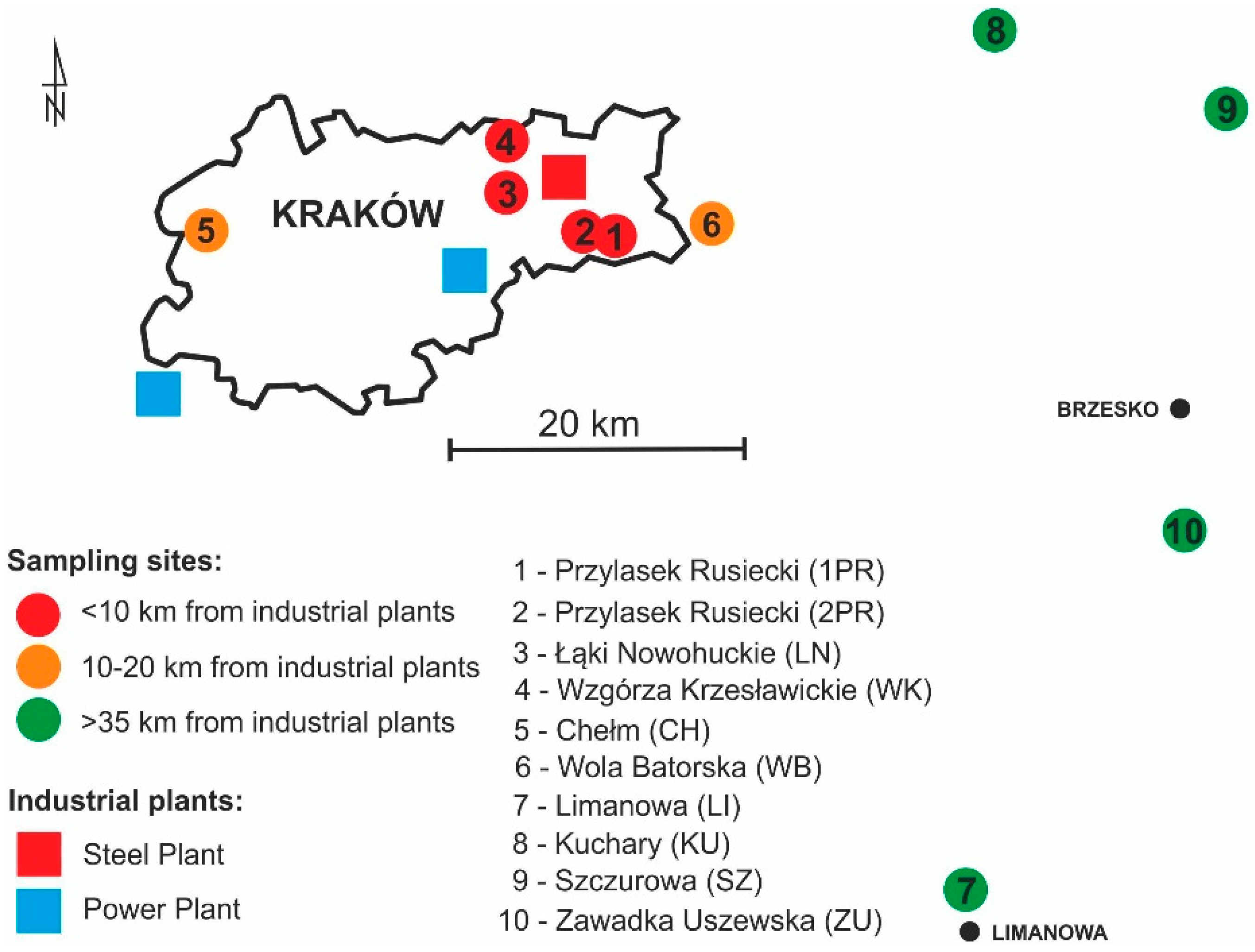
2. Experiments
3. Results and Discussion
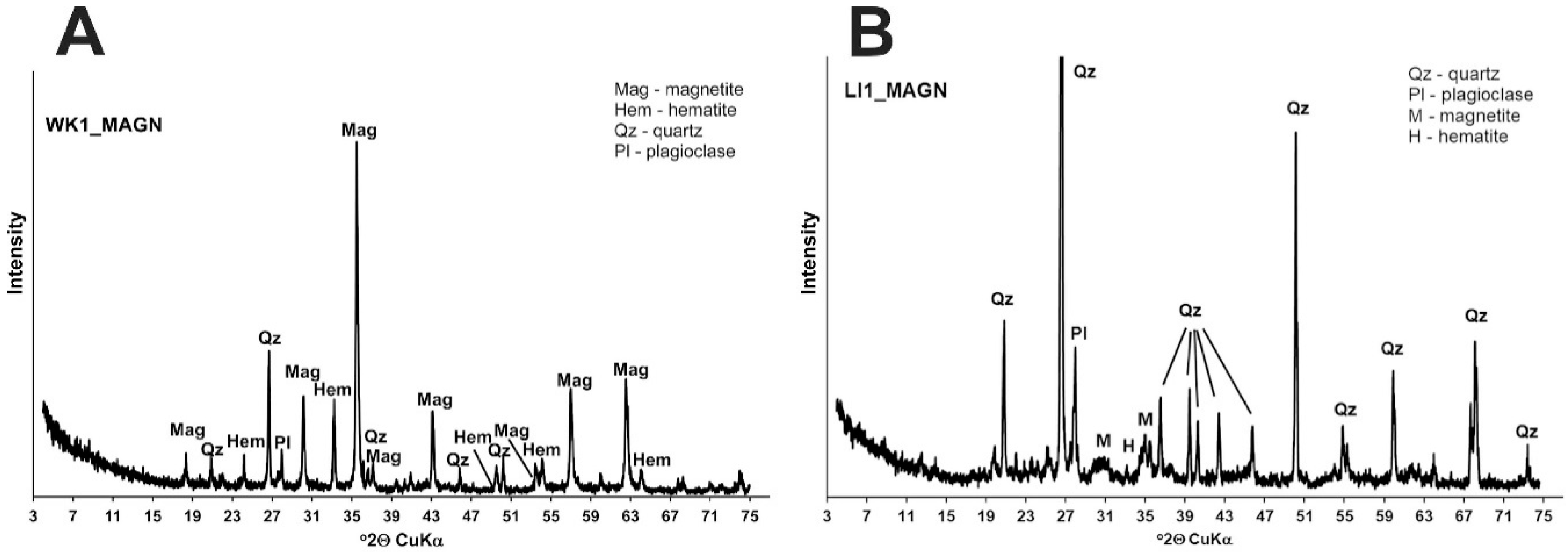
3.1. Mineral Composition of Soil Samples
3.2. Chemical Composition of Soil Samples
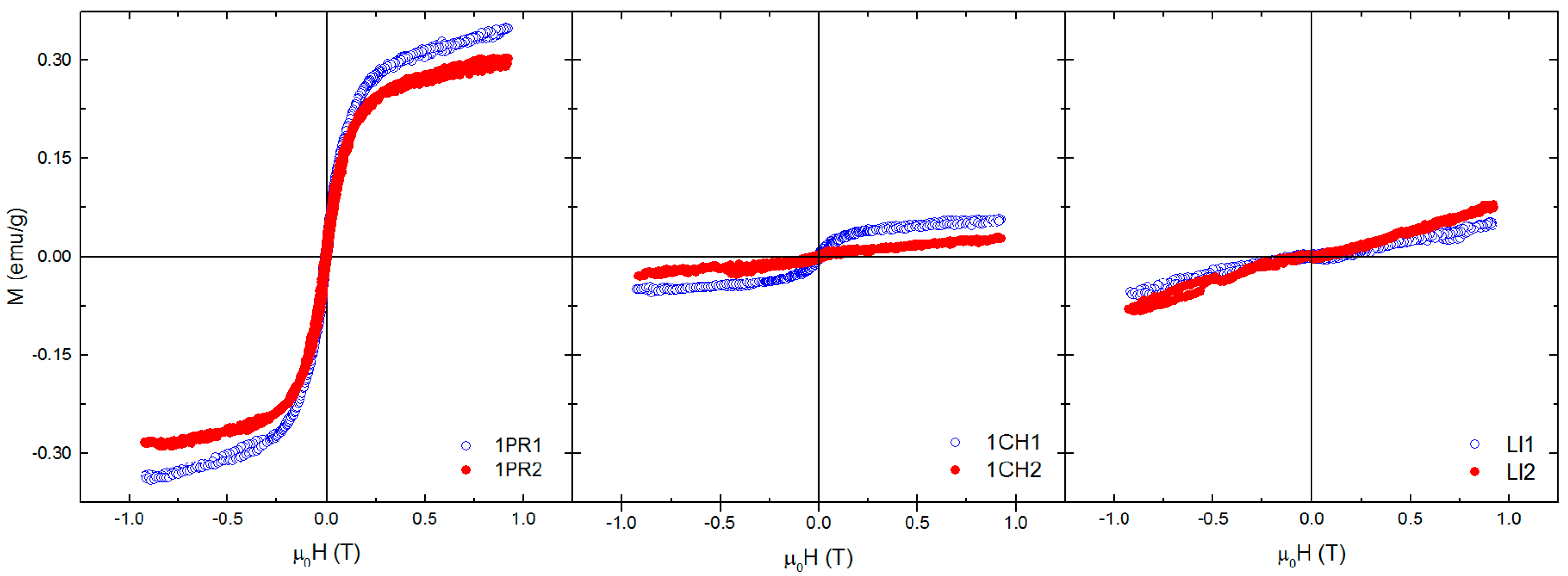
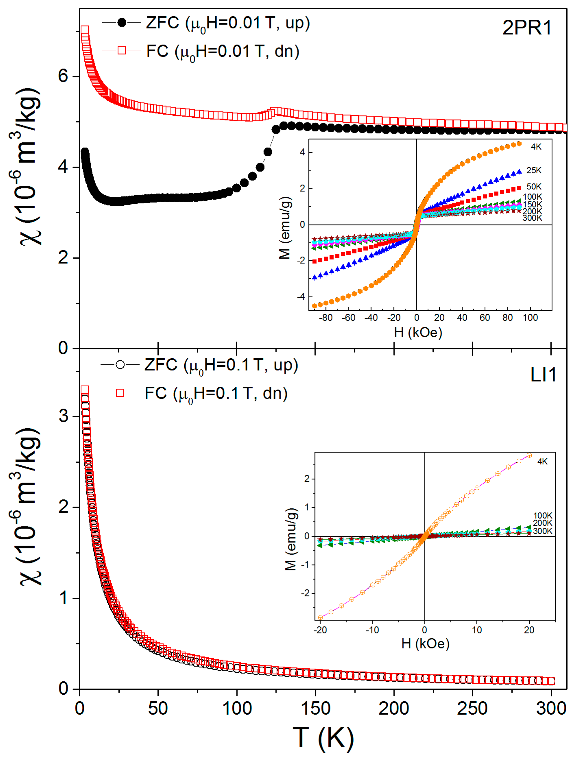
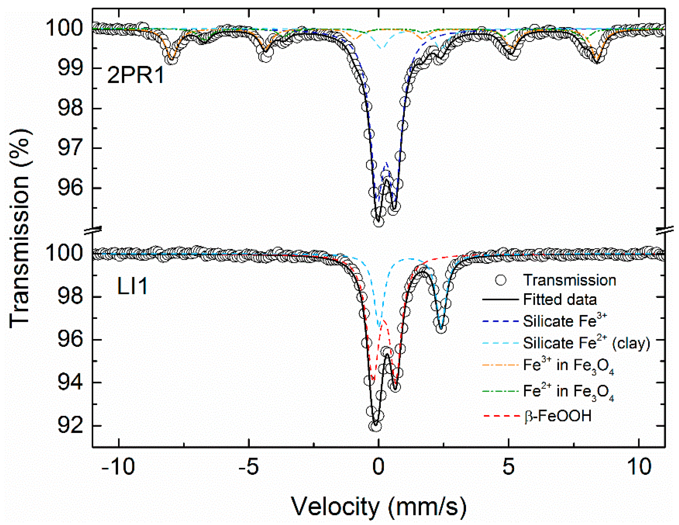
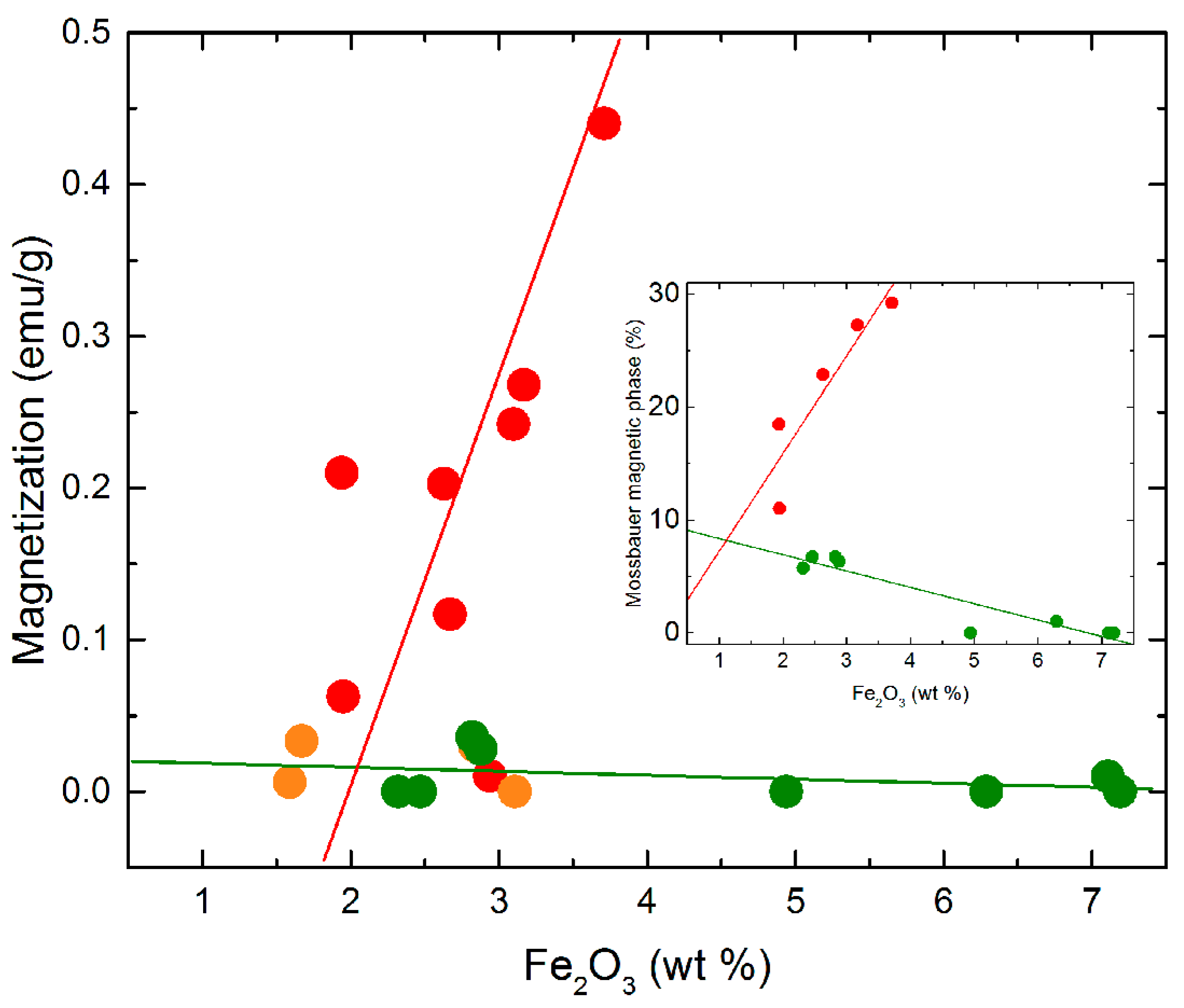
3.3. Magnetic Properties of Soil Samples and Mössbauer Spectroscopy
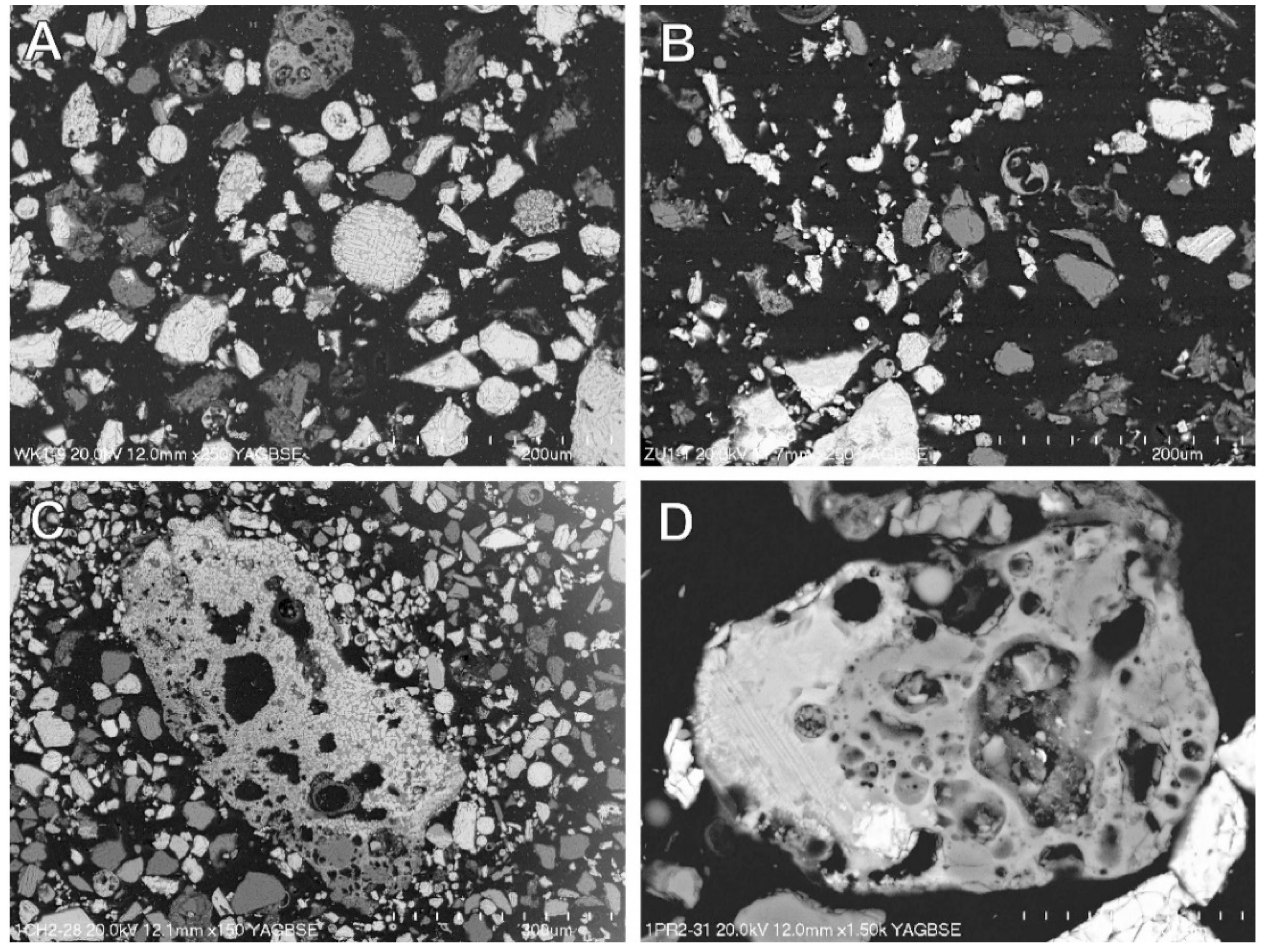
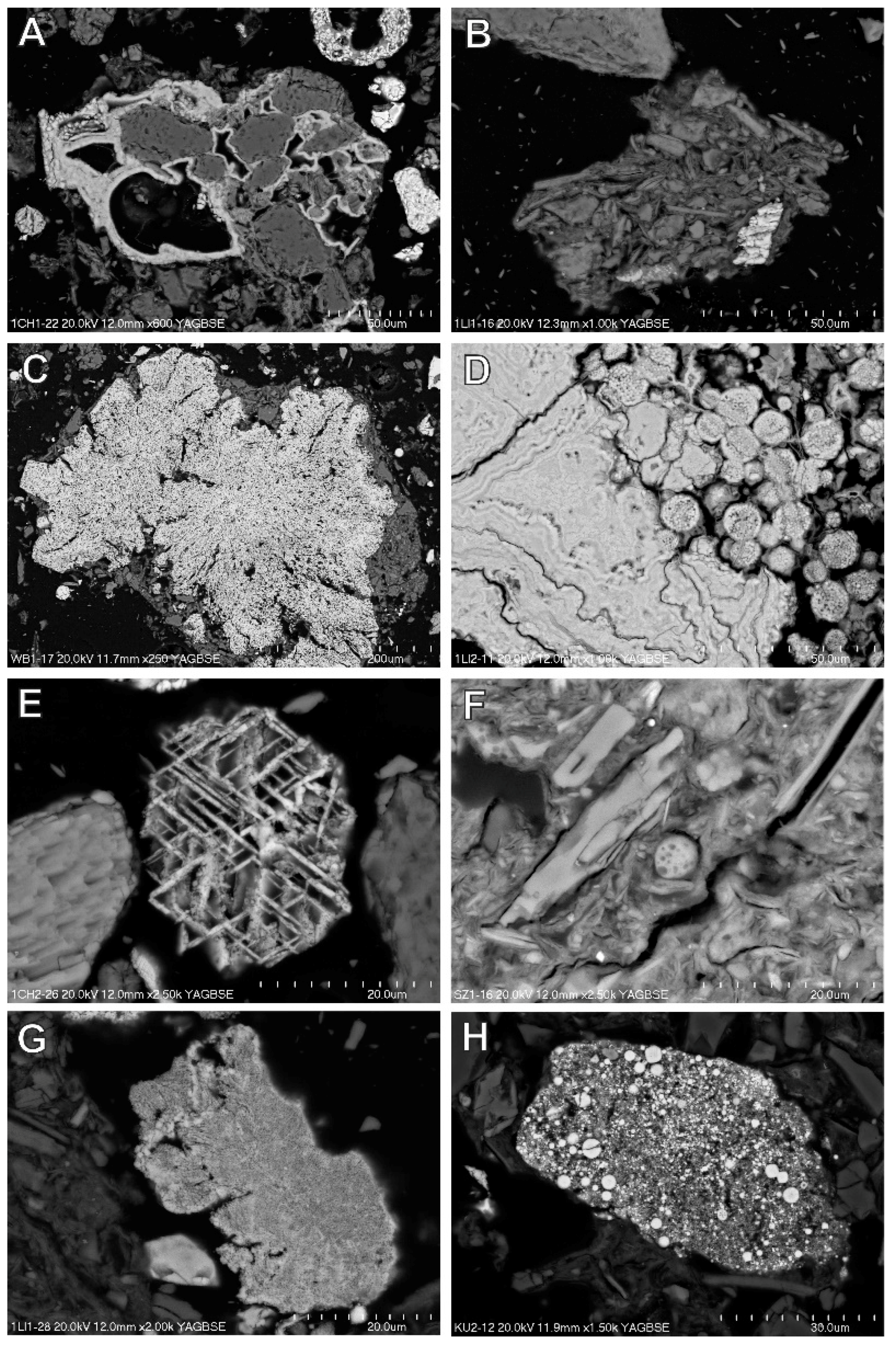
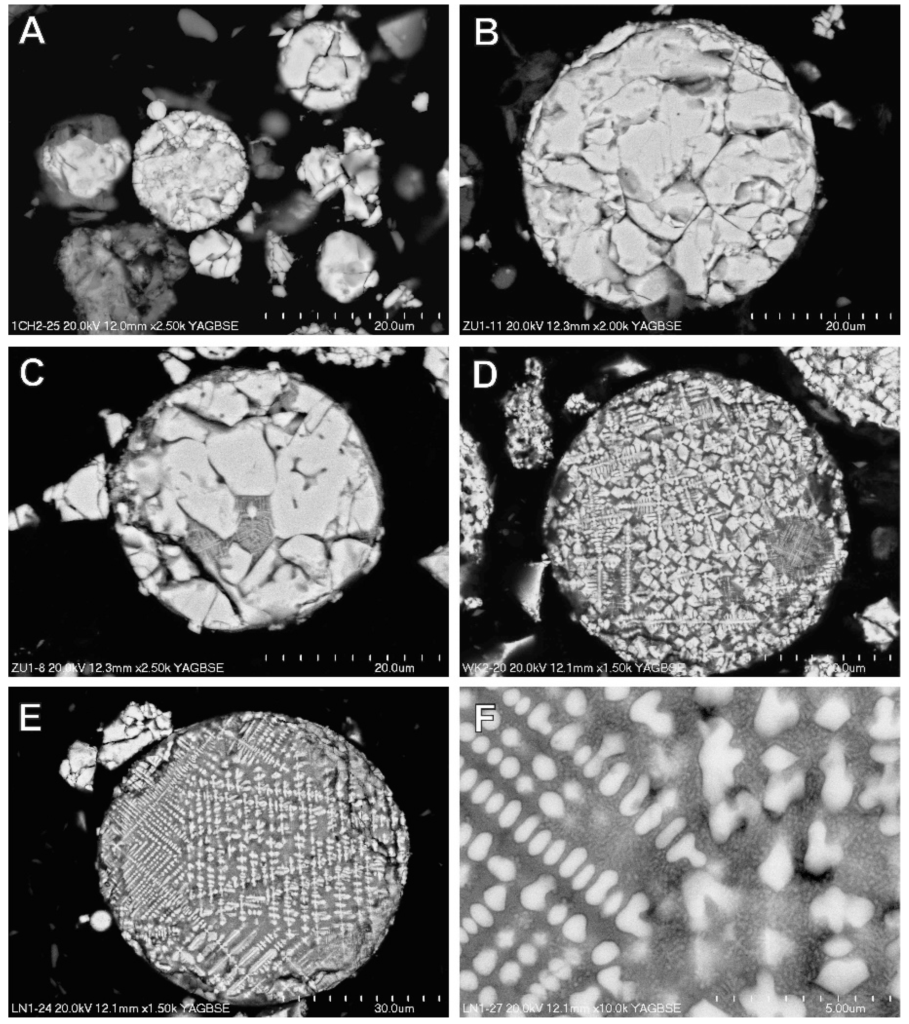
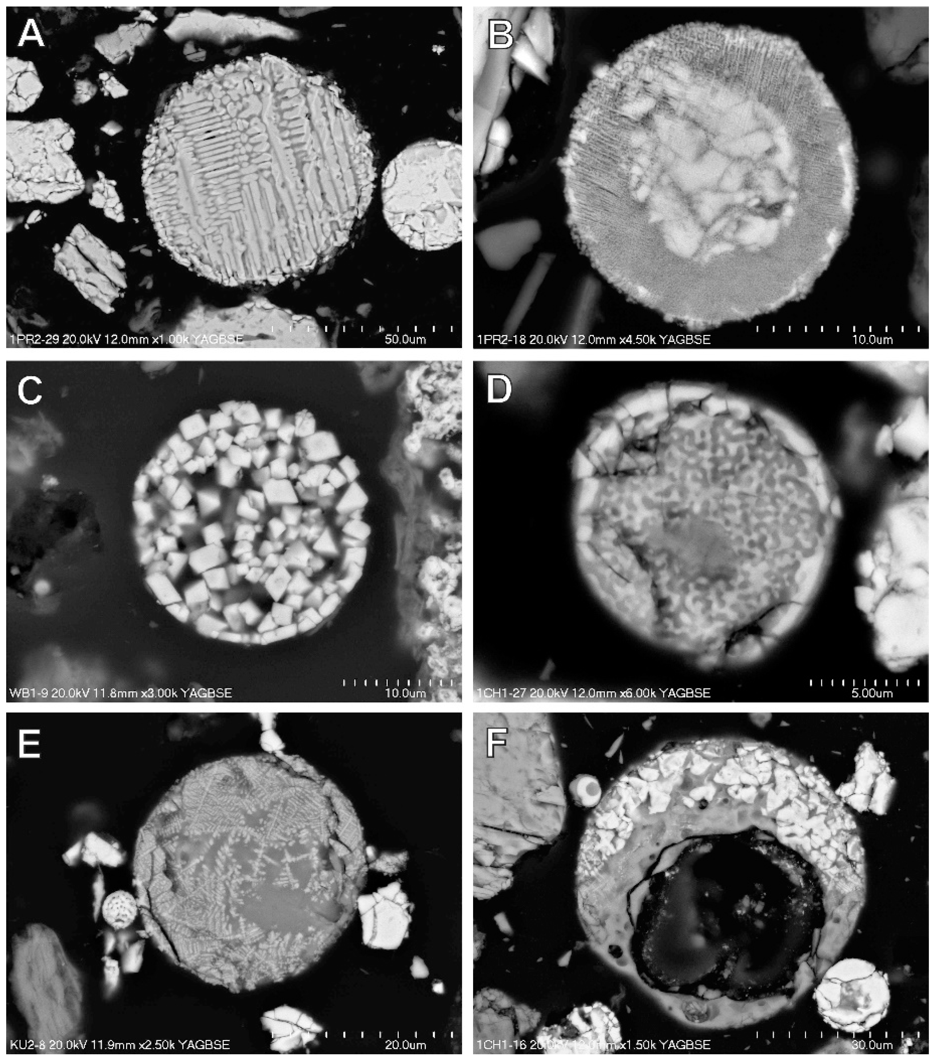
3.4. Magnetic Fraction Characteristics
4. Conclusions
Author Contributions
Funding
Acknowledgments
Conflicts of Interest
References
- Crutzen, P.J.; Stoermer, E.F. The “Anthropocene”. Glob. Chang. Newsl. 2000, 41, 17–18. [Google Scholar]
- Crutzen, P.J. Geology of mankind. Nature 2002, 415, 23. [Google Scholar] [CrossRef] [PubMed]
- Zalasiewicz, J.; Waters, C.N.; Williams, M.; Barnosky, A.D.; Cearreta, A.; Crutzen, P.; Ellis, E.; Ellis, M.A.; Fairchild, I.J.; Grinevald, J.; et al. When did the Anthropocene begin? A mid-twentieth century boundary level is stratigraphically optimal. Quat. Int. 2015, 383, 196–203. [Google Scholar] [CrossRef]
- Zalasiewicz, J.; Kryza, R.; Williams, M. The mineral signature of the Anthropocene in its DEEP-time Context. In A Stratigraphical Basis for the Anthropocene; Waters, C.N., Zalasiewicz, J.A., Williams, M., Ellis, M.A., Snelling, A.M., Eds.; Geological Society: London, UK, 2014; Volume 395, pp. 109–117. [Google Scholar]
- Zalasiewicz, J.; Waters, C.; Williams, M.; Aldridge, D.C.; Wilkinson, I.P. The stratigraphical signature of the Anthropocene in England and its wider context. Proc. Geol. Assoc. 2018, 129, 482–491. [Google Scholar] [CrossRef]
- Goudie, A.S. Dust storms: Recent developments. J. Environ. Manag. 2019, 90, 89–94. [Google Scholar] [CrossRef] [PubMed]
- Gałuszka, A.; Migaszewski, Z.M.; Zalasiewicz, J. Assessing the Anthropocene with geochemical methods. In A Stratigraphical Basis for the Anthropocene; Waters, C.N., Zalasiewicz, J.A., Williams, M., Ellis, M.A., Snelling, A.M., Eds.; Geological Society: London, UK, 2014; Volume 395, pp. 221–238. [Google Scholar]
- Gałuszka, A.; Migaszewski, Z.M.; Namieśnik, J. The role of analytical chemistry in the study of the Anthropocene. Trends Anal. Chem. 2017, 97, 146–152. [Google Scholar] [CrossRef]
- Marx, S.K.; Rashid, S.; Stromsoe, N. Global-scale patterns in anthropogenic Pb contamination reconstructed from natural archives. Environ. Pollut. 2014, 213, 283–298. [Google Scholar] [CrossRef]
- Rudnick, R.L.; Gao, S. The composition of the continental crust. In Treatise on Geochemistry–The Crust; Rudnick, R.L., Holland, H.D., Turekian, K.K., Eds.; Elsevier: Oxford, UK, 2003; pp. 1–64. [Google Scholar]
- Waters, C.N.; Zalasiewicz, J.; Summerhayes, C.; Fairchild, I.J.; Rose, N.L.; Loader, N.J.; Shotyk, W.; Cearreta, A.; Head, M.J.; Syvitski, J.P.M.; et al. Global Boundary Stratotype Section and Point (GSSP) for the Anthropocene Series: Where and how to look for potential candidates. Earth Sci. Rev. 2018, 178, 379–429. [Google Scholar] [CrossRef]
- Oldfield, F. Can the magnetic signatures from inorganic fly ash be used to mark the onset of the Anthropocene? Anthr. Rev. 2015, 2, 3–13. [Google Scholar] [CrossRef]
- Wilczyńska-Michalik, W.; Michalik, J.; Zimirska, A.; Kuca, A.; Dietrich, A.; Michalik, M. Magnetic technoparticles in soil as a record of Anthropocene. In Proceedings of the Goldschmidt2017 Abstract, Paris, France, 13–18 August 2017. [Google Scholar]
- Lu, S.G.; Bai, S.Q. Study on the correlation of magnetic properties and heavy metals content in urban soils of Hangzhou City, China. J. Appl. Geophys. 2016, 60, 1–12. [Google Scholar] [CrossRef]
- Magiera, T.; Mendakiewicz, M.; Szuszkiewicz, M.; Jab, M.; Chróst, L. Science of the Total Environment Technogenic magnetic particles in soils as evidence of historical mining and smelting activity: A case of the Brynica River Valley, Poland. Sci. Total Environ. 2016, 566–567, 536–551. [Google Scholar] [CrossRef] [PubMed]
- Łuczak, K.; Kusza, G. Magnetic Susceptibility in the Soils along Communication Routes in the Town of Opole. J. Ecol. Eng. 2019, 20, 234–238. [Google Scholar] [CrossRef]
- Magiera, T.; Go, B.; Jab, M. Technogenic Magnetic Particles in Alkaline Dusts from Power and Cement Plants. Water Air Soil Pollut. 2013, 224, 1389. [Google Scholar] [CrossRef] [PubMed]
- Szuszkiewicz, M.; Łukasik, A.; Magiera, T.; Mendakiewicz, M. Combination of geo- pedo- and technogenic magnetic and geochemical signals in soil profiles - Diversification and its interpretation: A new approach. Environ. Pollut. 2016, 214, 464–477. [Google Scholar] [CrossRef]
- Thompson, R. Environmental Magnetism; Allen & Unwin: London, UK, 1986. [Google Scholar]
- Singer, M.J.; Fine, P. Pedogenic Factors Affecting Magnetic Susceptibility of Northern California Soils. Soil Sci. Soc. Am. J. 1989, 53, 1119. [Google Scholar] [CrossRef]
- Loveland, P.J. Magnetic susceptibility of soil: An evaluation of conflicting theories using a national data set. Geophys. J. Int. 1996, 127, 728–734. [Google Scholar]
- Gangas, N.; Simopoulos, A.; Kostikas, A.; Yassoglou, N.; Filippakis, S. Mössbauer Studies of Small Particles of Iron Oxides in Soil. Clays Clay Miner. 1973, 21, 151–160. [Google Scholar] [CrossRef]
- Mijovilovich, A.; Saragovi, C. Evidences of the stability of magnetite in soil from Northeastern Argentina by Mössbauer spectroscopy and magnetization measurements. Phys. B Condens. Matter 2004, 354, 373–376. [Google Scholar] [CrossRef]
- Jeleńska, M.; Hasso-Agopsowicz, A.; Kopcewicz, B. Thermally induced transformation of magnetic minerals in soil based on rock magnetic study and Mössbauer analysis. Phys. Earth Planet. Inter. 2010, 179, 164–177. [Google Scholar] [CrossRef]
- Necula, C.; Panaiotu, C.; Schinteie, G.; Palade, C.; Kuncser, V. Reconstruction of superparamagnetic particle grain size distribution from Romanian loess using frequency dependent magnetic susceptibility and temperature dependent Mössbauer spectroscopy. Glob. Planet. Chang. 2015, 131, 89–103. [Google Scholar] [CrossRef]
- Kopcewicz, B.; Kopcewicz, M. Ecological aspects of Mössbauer study of iron-containing atmospheric aerosols. Hyperfine Interact. 2000, 126, 131–135. [Google Scholar] [CrossRef]
- Lu, S.; Yu, X.; Chen, Y. Science of the Total Environment Magnetic properties, microstructure and mineralogical phases of technogenic magnetic particles (TMPs) in urban soils: Their source identification and environmental implications. Sci. Total Environ. 2016, 543, 239–247. [Google Scholar] [CrossRef] [PubMed]
- Matuszko, D.; Piotrowicz, K.; Kowanetz, L. Klimat [Climate]. In Natural Environment of Krakow, Resources–Protection–Management; Baścik, M., Degórska, B., Eds.; Institute of Geography and Spatial Management, Jagiellonian University in Krakow: Kraków, Poland, 2015; pp. 81–108. [Google Scholar]
- Garścia, E. Wprowadzenie do dyskusji. In Problemy Ekologiczne Krakowa, 18, Atmosfera nad Krakowem, Przeszłość, Teraźniejszość, Przyszłość; Wydawnictwa AGH: Kraków, Poland, 1995; pp. 33–35. [Google Scholar]
- Tomlinson, D.L.; Wilson, J.G.; Harris, C.R.; Jeffrey, D.W. Problems in the assessment of heavy-metal levels in estuaries and the formation of a pollution index. Helgoländer Meeresunters. 1980, 33, 566–575. [Google Scholar] [CrossRef]
- Locke, G.; Bertine, K.K. Magnetite in sediments as an indicator of coal combustion. Appl. Geochem. 1986, 1, 345–356. [Google Scholar] [CrossRef]
- Veneva, L.; Hoffmann, V.; Jordanova, D.; Jordanova, N.; Fehr, T. Rock magnetic, mineralogical and microstructural characterization of fly ashes from Bulgarian power plants and the nearby anthropogenic soils. Phys. Chem. Earth 2004, 29, 1011–1023. [Google Scholar] [CrossRef]
- Vu, D.-H.; Bui, H.-B.; Kalantar, B.; Bui, X.-N.; Nguyen, D.-A.; Le, Q.-T.; Do, N.-H.; Nguyen, H. Composition and Morphology Characteristics of Magnetic Fractions of Coal Fly Ash Wastes Processed in High-Temperature Exposure in Thermal Power Plants. Appl. Sci. 2019, 9, 1964. [Google Scholar] [CrossRef]
- Murtha, M.J.; Burnet, G. The Magnetic Fraction of Coal Fly Ash: Its Separation, Properties, and Utilization. Proc. Iowa Acad. Sci. 1978, 85, 10–13. [Google Scholar]
- Li, J.; Zhu, J.; Qiao, S.; Yu, Z.; Wang, X.; Liu, Y.; Meng, X. Processing of coal fly ash magnetic spheres for clay water flocculation. Int. J. Miner. Process. 2017, 169, 162–167. [Google Scholar] [CrossRef]
- Valeev, D.; Kunilova, I.; Alpatov, A.; Varnavskaya, A.; Ju, D. Magnetite and Carbon Extraction from Coal Fly Ash Using Magnetic Separation and Flotation Methods. Minerals 2019, 9, 320. [Google Scholar] [CrossRef]
- Wilczyńska-Michalik, W. Z badań mineralogicznych pyłów emitowanych przez Hutę im. Lenina w Krakowie [Mineralogical study of dusts emitted from the Lenin Steel Plant in Kraków]. Prace Mineralogiczne PAN 1981, 68, 1–57. [Google Scholar]
- Muszer, A. Mineralogical characteristics of metallurgical dust in the vicinity of Głogów. Physicochem. Probl. Miner. Process. 2004, 38, 329–340. [Google Scholar]
- Csavina, J.; Taylor, M.P.; Félix, O.; Rine, K.P.; Sáez, A.E.; Betterton, E.A. Size-resolved dust and aerosol contaminants associated with copper and lead smelting emissions: Implications for emissions management and human health. Sci. Total Environ. 2014, 493, 750–756. [Google Scholar] [CrossRef] [PubMed]
- Yang, T.; Liu, Q.; Zeng, Q.; Chan, L. Relationship between magnetic properties and heavy metals of urban soils with different soil types and environmental settings: Implications for magnetic mapping. Environ. Earth Sci. 2012, 66, 409–420. [Google Scholar] [CrossRef]


| Sample | Component (wt%) | |||||||||||||
|---|---|---|---|---|---|---|---|---|---|---|---|---|---|---|
| SiO2 | Al2O3 | Fe2O3 | MnO | MgO | CaO | Na2O | K2O | TiO2 | P2O5 | LOI | Total | Ctot | Stot | |
| 1PR1 | 73.31 | 7.60 | 3.17 | 0.09 | 0.59 | 1.10 | 0.80 | 2.19 | 0.64 | 0.30 | 10.10 | 99.89 | 3.72 | 0.04 |
| 1PR2 | 76.25 | 7.69 | 3.10 | 0.10 | 0.58 | 1.25 | 0.83 | 2.19 | 0.65 | 0.26 | 6.80 | 99.7 | 2.07 | 0.03 |
| 2PR1 | 65.34 | 7.58 | 3.71 | 0.08 | 0.65 | 1.57 | 0.76 | 1.89 | 0.57 | 0.22 | 17.4 | 99.77 | 6.63 | 0.09 |
| 2PR2 | 74.02 | 8.30 | 2.94 | 0.04 | 0.58 | 1.07 | 0.84 | 1.86 | 0.64 | 0.14 | 9.30 | 99.73 | 2.29 | 0.03 |
| WK1 | 78.83 | 7.58 | 2.63 | 0.07 | 0.50 | 0.66 | 0.81 | 2.11 | 0.67 | 0.12 | 5.80 | 99.78 | 2.72 | 0.03 |
| WK2 | 76.56 | 7.21 | 2.67 | 0.06 | 0.47 | 0.69 | 0.78 | 2.02 | 0.66 | 0.14 | 8.50 | 99.76 | 1.50 | <0.02 |
| LN1 | 83.83 | 3.91 | 1.94 | 0.03 | 0.26 | 0.57 | 0.31 | 1.00 | 0.28 | 0.12 | 7.60 | 99.85 | 3.05 | 0.04 |
| LN2 | 84.21 | 4.76 | 1.95 | 0.03 | 0.30 | 0.60 | 0.36 | 1.12 | 0.35 | 0.1 | 6.10 | 99.88 | 1.99 | 0.03 |
| CH1 | 81.81 | 6.34 | 1.67 | 0.06 | 0.34 | 0.37 | 0.74 | 1.92 | 0.65 | 0.12 | 5.70 | 99.72 | 1.71 | <0.02 |
| CH2 | 83.73 | 6.51 | 1.59 | 0.06 | 0.35 | 0.38 | 0.75 | 1.92 | 0.67 | 0.08 | 3.70 | 99.74 | 0.78 | <0.02 |
| WB1 | 74.42 | 8.27 | 2.84 | 0.09 | 0.62 | 0.47 | 0.91 | 1.79 | 0.67 | 0.15 | 9.60 | 99.83 | 2.69 | 0.03 |
| WB2 | 76.79 | 9.02 | 3.11 | 0.10 | 0.69 | 0.45 | 1.00 | 1.99 | 0.74 | 0.16 | 5.80 | 99.85 | 0.95 | <0.02 |
| SZ1 | 55.82 | 13.30 | 7.11 | 0.26 | 1.08 | 0.62 | 0.53 | 1.74 | 0.74 | 0.20 | 18.40 | 99.8 | 3.96 | 0.05 |
| SZ2 | 62.47 | 14.12 | 7.19 | 0.45 | 1.17 | 0.75 | 0.65 | 2.14 | 0.76 | 0.09 | 10.00 | 99.79 | 0.73 | <0.02 |
| KU1 | 72.14 | 8.22 | 2.82 | 0.06 | 0.72 | 1.53 | 0.82 | 2.31 | 0.67 | 0.20 | 10.30 | 99.79 | 3.48 | 0.04 |
| KU2 | 76.16 | 8.52 | 2.88 | 0.06 | 0.74 | 1.20 | 0.83 | 2.34 | 0.69 | 0.16 | 6.20 | 99.78 | 1.81 | 0.02 |
| LI1 | 65.88 | 13.63 | 4.94 | 0.10 | 1.50 | 0.46 | 1.17 | 2.63 | 0.93 | 0.13 | 8.40 | 99.77 | 1.79 | 0.03 |
| LI2 | 63.99 | 15.50 | 6.29 | 0.19 | 1.83 | 0.37 | 1.21 | 3.00 | 0.86 | 0.08 | 6.50 | 99.82 | 0.54 | <0.02 |
| ZU1 | 78.48 | 7.84 | 2.32 | 0.06 | 0.53 | 0.41 | 0.80 | 2.10 | 0.69 | 0.09 | 6.50 | 99.82 | 1.72 | 0.02 |
| ZU2 | 79.73 | 8.38 | 2.47 | 0.08 | 0.56 | 0.43 | 0.85 | 2.23 | 0.76 | 0.10 | 4.20 | 99.79 | 0.66 | <0.02 |
| Sample | Element | |||||||||||||||||||||||
| Ag | As * | Au ** | Ba | Be | Bi | Cd * | Co * | Cr * | Cs | Cu * | Ga | Hf | Hg | Mo | Nb | Ni * | Pb * | Rb | Sb | Sc | Se | Sn | Sr | |
| 1PR1 | <0.1 | 3.8 | 4.1 | 435 | <1 | 0.2 | 0.8 | 5.7 | 55.71 | 2.60 | 29.20 | 7.10 | 13.40 | 0.05 | 0.4 | 11.3 | 16.4 | 27.4 | 78.4 | 0.3 | 7 | <0.5 | 2 | 84.5 |
| 1PR2 | <0.1 | 4.6 | 1.9 | 439 | 2 | 0.2 | 1.1 | 6.7 | 61.90 | 3.00 | 32.20 | 7.70 | 14.00 | 0.06 | 0.3 | 12.4 | 16.9 | 32.0 | 86.6 | 0.3 | 7 | <0.5 | 3 | 96.4 |
| 2PR1 | <0.1 | 4.6 | 5.7 | 389 | 1 | 0.2 | 1.4 | 6.0 | 74.29 | 2.60 | 19.10 | 7.60 | 10.10 | 0.07 | 0.4 | 10.7 | 16.9 | 41.8 | 66.2 | 0.4 | 7 | <0.5 | 2 | 86.8 |
| 2PR2 | <0.1 | 4.6 | 5.0 | 429 | <1 | 0.1 | 0.6 | 6.3 | 61.90 | 3.00 | 14.70 | 7.80 | 13.80 | 0.04 | <0.1 | 12.5 | 17.6 | 24.9 | 64.5 | 0.2 | 7 | 0.5 | 2 | 89.9 |
| WK1 | <0.1 | 4.4 | 4.1 | 426 | 1 | 0.1 | 0.7 | 7.4 | 49.52 | 2.60 | 14.90 | 7.20 | 15.00 | 0.05 | 0.3 | 13.0 | 13.5 | 27.6 | 75.0 | 0.4 | 7 | 0.7 | 2 | 89.2 |
| WK2 | <0.1 | 5.0 | 9.7 | 428 | <1 | 0.2 | 1.2 | 6.5 | 49.52 | 2.50 | 16.30 | 6.70 | 14.90 | 0.07 | 0.4 | 13.1 | 13.2 | 35.2 | 72.4 | 0.4 | 6 | <0.5 | 2 | 88.8 |
| LN1 | <0.1 | 4.8 | 3.7 | 244 | 2 | 0.1 | 0.8 | 3.9 | 43.33 | 1.60 | 9.30 | 2.80 | 5.60 | 0.04 | 0.3 | 5.3 | 7.5 | 29.2 | 34.1 | 0.9 | 3 | <0.5 | 1 | 48.4 |
| LN2 | 0.1 | 5.2 | 2.3 | 262 | <1 | <0.1 | 0.7 | 4.7 | 30.95 | 1.50 | 10.30 | 4.60 | 6.50 | 0.03 | 0.1 | 6.5 | 9.5 | 26.5 | 39.9 | 0.5 | 4 | <0.5 | 2 | 52.0 |
| CH1 | <0.1 | 3.1 | 2.8 | 363 | 2 | 0.1 | 0.7 | 4.9 | 61.90 | 1.90 | 6.60 | 6.10 | 15.80 | 0.03 | 0.2 | 12.0 | 7.5 | 27.6 | 64.5 | 0.2 | 5 | 0.5 | 2 | 69.6 |
| CH2 | <0.1 | 2.6 | 2.2 | 370 | <1 | 0.1 | 0.7 | 4.2 | 55.71 | 1.70 | 6.00 | 5.60 | 15.60 | 0.03 | 0.2 | 12.2 | 7.8 | 23.1 | 64.5 | 0.2 | 5 | <0.5 | 1 | 69.5 |
| WB1 | 0.1 | 5.3 | 4.1 | 387 | 2 | 0.2 | 0.9 | 6.7 | 74.29 | 3.00 | 15.50 | 8.50 | 11.80 | 0.07 | 0.30 | 12.90 | 26.00 | 34.00 | 87.6 | 0.30 | 7 | <0.5 | 3 | 72.6 |
| WB2 | <0.1 | 5.1 | 3.1 | 433 | <1 | 0.2 | 0.7 | 8.2 | 80.48 | 3.50 | 14.50 | 9.60 | 11.80 | 0.05 | 0.20 | 14.10 | 29.00 | 27.30 | 92.4 | 0.20 | 8 | <0.5 | 2 | 79.3 |
| SZ1 | 0.1 | 15.2 | 4.9 | 414 | 2 | 0.4 | 0.6 | 15.7 | 80.48 | 7.40 | 19.90 | 15.80 | 6.40 | 0.07 | 0.90 | 13.80 | 35.00 | 44.00 | 131.7 | 0.20 | 12 | 1 | 3 | 80.3 |
| SZ2 | <0.1 | 11.6 | 6.4 | 518 | <1 | 0.3 | 0.4 | 24.5 | 80.48 | 7.40 | 24.60 | 16.30 | 8.80 | 0.06 | 0.80 | 14.40 | 46.00 | 21.90 | 122.7 | 0.10 | 13 | 0.8 | 3 | 89.5 |
| KU1 | <0.01 | 4.8 | 14.5 | 386 | 2 | 0.1 | 0.5 | 6.8 | 55.71 | 2.80 | 16.50 | 8.30 | 14.70 | 0.04 | 0.40 | 12.30 | 22.00 | 26.20 | 78.7 | 0.30 | 7 | 0.7 | 2 | 86.9 |
| KU2 | <0.01 | 5.6 | 2.3 | 403 | 2 | 0.2 | 0.5 | 7.1 | 55.71 | 3.00 | 14.70 | 9.40 | 15.30 | 0.05 | 0.20 | 13.40 | 22.00 | 22.90 | 86.4 | 0.20 | 7 | 0.5 | 2 | 85.1 |
| LI1 | <0.1 | 6.0 | 4.1 | 457 | <1 | 0.3 | 0.6 | 14.9 | 92.86 | 5.60 | 23.10 | 15.50 | 8.40 | 0.09 | 0.7 | 17.5 | 37.9 | 31.5 | 116.5 | 0.2 | 13 | 0.6 | 3 | 99.5 |
| LI2 | <0.1 | 8.7 | 21.9 | 459 | 4 | 0.3 | 0.2 | 20.4 | 99.05 | 5.90 | 33.50 | 18.00 | 7.10 | 0.04 | 0.8 | 15.4 | 49.9 | 24.9 | 127.2 | 0.2 | 15 | <0.5 | 3 | 89.9 |
| ZU1 | <0.1 | 5.2 | 3.7 | 409 | <1 | 0.2 | 0.2 | 6.6 | 55.71 | 2.80 | 10.60 | 8.70 | 16.10 | 0.07 | 0.30 | 13.80 | <20 | 17.80 | 82.3 | 0.20 | 6 | <0.5 | 2 | 78.9 |
| ZU2 | <0.1 | 4.1 | 3.8 | 431 | 2 | 0.1 | 0.2 | 6.9 | 55.71 | 3.00 | 9.20 | 8.30 | 17.10 | 0.04 | 0.50 | 15.00 | 21.00 | 16.40 | 85.9 | 0.20 | 7 | <0.5 | 2 | 79.4 |
| Sample | Element | |||||||||||||||||||||||
| Ta | Th | Tl | U | V | W | Y | Zn * | Zr | La | Ce | Pr | Nd | Sm | Eu | Gd | Tb | Dy | Ho | Er | Tm | Yb | Lu | PLI *** | |
| 1PR1 | <0.1 | 9.1 | 0.2 | 2.7 | 52.0 | 1.7 | 24.0 | 140 | 500.1 | 27.6 | 56.8 | 6.93 | 26.00 | 4.89 | 0.80 | 4.35 | 0.72 | 4.40 | 0.84 | 2.53 | 0.41 | 2.68 | 0.46 | 1.055 |
| 1PR2 | <0.1 | 8.9 | 0.2 | 2.8 | 51.0 | 2.1 | 27.0 | 156 | 545.9 | 29.5 | 59.1 | 6.94 | 26.50 | 5.04 | 0.94 | 4.85 | 0.80 | 4.75 | 0.91 | 2.81 | 0.43 | 3.02 | 0.47 | 1.221 |
| 2PR1 | <0.1 | 8.5 | 0.1 | 2.4 | 49.0 | 1.4 | 23.7 | 176 | 394.6 | 24.3 | 50.9 | 6.06 | 21.70 | 4.74 | 0.85 | 4.32 | 0.72 | 3.92 | 0.78 | 2.54 | 0.39 | 2.63 | 0.42 | 1.249 |
| 2PR2 | <0.1 | 10.4 | <0.1 | 2.9 | 51.0 | 1.3 | 25.9 | 80 | 526.9 | 28.8 | 59.5 | 6.90 | 25.20 | 4.99 | 0.93 | 4.93 | 0.78 | 4.49 | 0.89 | 2.83 | 0.44 | 2.94 | 0.46 | 0.913 |
| WK1 | <0.1 | 9.4 | 0.2 | 3.0 | 48.0 | 1.6 | 27.4 | 101 | 594.2 | 28.7 | 58.4 | 6.69 | 25.80 | 4.89 | 0.86 | 4.73 | 0.77 | 4.66 | 0.96 | 3.18 | 0.49 | 3.19 | 0.51 | 0.928 |
| WK2 | <0.1 | 9.2 | 0.2 | 3.3 | 46.0 | 3.1 | 26.9 | 139 | 578.1 | 26.8 | 58.5 | 6.82 | 26.10 | 5.05 | 0.84 | 4.73 | 0.80 | 4.67 | 0.89 | 2.99 | 0.46 | 3.16 | 0.49 | 1.074 |
| LN1 | <0.1 | 4.2 | <0.1 | 1.6 | 23.0 | 1.8 | 11.5 | 124 | 213.6 | 12.3 | 26.2 | 2.86 | 11.10 | 2.22 | 0.38 | 1.98 | 0.32 | 1.81 | 0.38 | 1.19 | 0.19 | 1.34 | 0.21 | 0.784 |
| LN2 | 0.1 | 5.3 | <0.1 | 1.7 | 31.0 | 0.7 | 13.2 | 83 | 253.7 | 15.9 | 32.0 | 3.61 | 12.50 | 2.39 | 0.46 | 2.28 | 0.39 | 2.15 | 0.45 | 1.37 | 0.21 | 1.48 | 0.22 | 0.749 |
| CH1 | <0.1 | 9.4 | 0.2 | 3.0 | 45.0 | 1.3 | 22.7 | 62 | 592.0 | 25.2 | 53.9 | 5.93 | 22.00 | 4.59 | 0.67 | 3.58 | 0.64 | 3.86 | 0.82 | 2.49 | 0.43 | 2.73 | 0.45 | 0.685 |
| CH2 | <0.1 | 9.3 | 0.1 | 2.8 | 36.0 | 2.3 | 22.5 | 64 | 601.2 | 24.9 | 51.8 | 5.71 | 20.20 | 4.06 | 0.66 | 3.78 | 0.63 | 3.96 | 0.80 | 2.67 | 0.38 | 2.66 | 0.43 | 0.632 |
| WB1 | 0.1 | 10.1 | 0.1 | 2.7 | 51.0 | 1.7 | 27.7 | 131.0 | 450.8 | 27.9 | 57.1 | 6.84 | 25.80 | 4.98 | 0.91 | 5.02 | 0.74 | 4.68 | 0.96 | 2.90 | 0.43 | 3.13 | 0.45 | 1.178 |
| WB2 | <0.1 | 11.4 | 0.1 | 2.9 | 57.0 | 1.5 | 27.6 | 104.0 | 456.8 | 32.5 | 66.8 | 8.01 | 31.50 | 5.6 | 1.02 | 5.29 | 0.81 | 4.74 | 1.00 | 3.11 | 0.45 | 3.02 | 0.46 | 1.118 |
| SZ1 | 0.1 | 12.3 | 0.3 | 3.2 | 107.0 | 1.9 | 25.1 | 126.0 | 241.3 | 32.3 | 66.4 | 7.86 | 30.40 | 5.56 | 1.11 | 5.21 | 0.75 | 4.80 | 0.92 | 2.70 | 0.41 | 2.59 | 0.41 | 1.579 |
| SZ2 | <0.1 | 13 | 0.3 | 3.6 | 110.0 | 1.7 | 31.2 | 88.0 | 322.6 | 35.1 | 85.1 | 8.99 | 33.40 | 6.63 | 1.35 | 6.53 | 0.95 | 5.68 | 1.15 | 3.50 | 1.49 | 3.20 | 0.52 | 1.428 |
| KU1 | <0.01 | 10.1 | 0.1 | 2.5 | 46.0 | 1.3 | 30.4 | 124.0 | 560.8 | 30.1 | 61.7 | 7.46 | 28.40 | 5.67 | 0.99 | 5.29 | 0.62 | 5.04 | 1.06 | 3.29 | 0.50 | 3.24 | 0.51 | 0.991 |
| KU2 | <0.01 | 10.7 | 0.1 | 2.8 | 51.0 | 1.1 | 31.3 | 73.0 | 595.8 | 31.4 | 65.4 | 8.04 | 30.30 | 5.69 | 1.06 | 5.64 | 0.85 | 5.41 | 1.12 | 3.39 | 0.48 | 3.39 | 0.52 | 0.921 |
| LI1 | <0.1 | 12 | 0.2 | 3.4 | 112.0 | 2.8 | 26.1 | 96 | 313.7 | 35.0 | 79.8 | 8.17 | 29.50 | 5.59 | 1.03 | 4.67 | 0.77 | 4.84 | 0.95 | 2.87 | 0.46 | 3.06 | 0.46 | 1.356 |
| LI2 | <0.1 | 12.4 | 0.1 | 3.1 | 122.0 | 2.1 | 22.6 | 84 | 257.3 | 33.3 | 74.9 | 7.85 | 28.10 | 4.99 | 1.00 | 4.27 | 0.72 | 4.26 | 0.89 | 2.68 | 0.42 | 2.70 | 0.44 | 1.344 |
| ZU1 | <0.1 | 11 | 0.1 | 3.0 | 44.0 | 1.8 | 29.7 | 49.0 | 612.2 | 31.2 | 65.4 | 7.58 | 27.30 | 5.33 | 0.93 | 5.01 | 0.80 | 5.17 | 1.08 | 3.31 | 0.50 | 3.42 | 0.53 | 0.441 |
| ZU2 | <0.1 | 11.8 | 0.1 | 3.4 | 47.0 | 1.8 | 30.3 | 40.0 | 657.4 | 32.9 | 70.0 | 8.09 | 30.20 | 5.66 | 0.92 | 5.39 | 0.82 | 5.15 | 1.10 | 3.41 | 0.49 | 3.38 | 0.52 | 0.657 |
| Sample | Content of Magnetic Fraction | Sample | Content of Magnetic Fraction |
|---|---|---|---|
| (wt%) | (wt%) | ||
| 1PR-1 | 0.90 | WB-1 | 0.19 |
| 1PR-2 | 0.90 | WB-2 | 0.03 |
| 2PR-1 | 4.80 | SZ-1 | 0.06 |
| 2PR-2 | 0.60 | SZ-2 | 0.03 |
| WK-1 | 2.27 | KU-1 | 0.70 |
| WK-2 | 1.55 | KU-2 | 0.29 |
| LN-1 | 10.87 | 1LI-1 | 0.09 |
| LN-2 | 1.16 | 1LI-2 | 0.07 |
| 1CH-1 | 0.30 | ZU-1 | 0.03 |
| 1CH-2 | 0.10 | ZU-2 | 0.05 |
© 2019 by the authors. Licensee MDPI, Basel, Switzerland. This article is an open access article distributed under the terms and conditions of the Creative Commons Attribution (CC BY) license (http://creativecommons.org/licenses/by/4.0/).
Share and Cite
Wilczyńska-Michalik, W.; Michalik, J.M.; Kapusta, C.; Michalik, M. Airborne Magnetic Technoparticles in Soils as a Record of Anthropocene. Atmosphere 2020, 11, 44. https://doi.org/10.3390/atmos11010044
Wilczyńska-Michalik W, Michalik JM, Kapusta C, Michalik M. Airborne Magnetic Technoparticles in Soils as a Record of Anthropocene. Atmosphere. 2020; 11(1):44. https://doi.org/10.3390/atmos11010044
Chicago/Turabian StyleWilczyńska-Michalik, Wanda, Jan M. Michalik, Czesław Kapusta, and Marek Michalik. 2020. "Airborne Magnetic Technoparticles in Soils as a Record of Anthropocene" Atmosphere 11, no. 1: 44. https://doi.org/10.3390/atmos11010044
APA StyleWilczyńska-Michalik, W., Michalik, J. M., Kapusta, C., & Michalik, M. (2020). Airborne Magnetic Technoparticles in Soils as a Record of Anthropocene. Atmosphere, 11(1), 44. https://doi.org/10.3390/atmos11010044