Precipitation Forecast Contribution Assessment in the Coupled Meteo-Hydrological Models

Abstract

A numerical weather prediction and a rainfall-runoff model employed to evaluate precipitation and flood forecast for the Imjin River (South and North Korea). The real-time precipitation at point and catchment scales evaluated to select proper hydrological model to couple with atmospheric model. As a major limitation of previous studies, temporal and spatial resolutions of hydrological model are smaller than those of meteorological model. Here, through high resolution of temporal (10 min) and spatial (1 km × 1 km), the optimal resolution determined. The results showed Weather Research and Forecasting (WRF) model underestimated precipitation in point and catchment assessment and its skill was relatively higher for catchment than point scale, as illustrated by the lower Root Mean Square Error (RMSE) of 59.67, 160.48, 68.49 for the catchment and 84.49, 212.80 and 91.53 for the point scale in the events 2002, 2007 and 2011, respectively. The findings led to choose the semi-distributed hydrological model. The variations in temporal and spatial resolutions illustrated accuracy decrease; additionally, the optimal spatial resolution obtained at 8 km and temporal resolution did not affect the inherent inaccuracy of the results. Lead-time variation demonstrated that lead-time dependency was almost negligible below 36 h. With reference to this study, comparisons of model performance provided quantitative knowledge for understanding credibility and restrictions of meteo-hydrological models.

1. Introduction

One of the most expensive natural disasters is due to severe floods, which are often triggered by heavy precipitation and increased by climate change and human activities [1]. The safety of lives and properties is always threatened by the severe floods. Meteo-hydrological predictions are important for providing early flood warnings and preventing or reducing flood damages [2,3]. The high resolution Numerical Weather Prediction (NWP) models provided notable improvement in Quantitative Precipitation Forecast (QPF). The QPF can be an alternative input data source for hydrological predictions. Coupling the NWP and hydrological models connects the progress in meteorology and hydrology to generate real-time flood forecasting. In one-way linking of meteorological and hydrological models, the atmospheric model outputs were extracted and used as input data for hydrological models. Although the application of the real-time precipitation of the NWP models grew in real-time flood forecasting, there is a vital need regarding the evaluation of the real-time precipitation forecast characteristics from NWP models.

As opposed to the increasing trend of the application of NWP models in coupling with hydrological models, there is no study for selecting the suitable type of the hydrological model. Hydrological model developments range from lumped to semi-distributed and fully distributed models. Within this wide range, the selection of the proper model for different purposes can be a difficult task, which depends on user experience and feasibility [4]. Since hydrological models are sensitive to the input data errors, for choosing a hydrological model for flood forecasting, the accuracy of the precipitation which is vast from the pixel and subbasin to the catchment scale plays a major role. Evaluation of point precipitation and the Mean Areal Precipitation (MAP) could lead to robust decision making in the distributed (which uses the point precipitation data as input) and semi-distributed (which uses the MAP as input) hydrological models. To clarify these aspects, the effect of precipitation errors on forecast flow is reported in previous studies [5,6].

In the evaluation of meteorological models, it has been found that atmospheric models have difficulty to forecast accurately their space-time evolution; therefore, atmospheric models predict the occurrence of the rainfall better than the magnitude and location of rainfall [7,8]. There are several errors in location, intensity and timing of the QPFs since the precise forecast of precipitation is one of the limitations of NWP models. Generally, NWP models overforecast light (1 mm) to moderate (5 mm) precipitation; however, they underforecast heavy precipitation in the Middle Atlantic Region (MAR) of the USA [9] as well as in the wet and high elevation areas of the Ovens catchment in Australia [10]. The use of WRF model in Korean peninsula showed underestimation of the precipitation amount [11]. There are many factors effected the quality of the QPF of the NWP models, the evaluation of forecast precipitation values indicated that the accuracy of rainfall forecast varies with the spatial resolution [12,13], temporal resolution [14,15] and lead-time [16,17] of meteorological models. The flood warnings improved by increasing the spatial resolution of the Met Office Unified Model (UM) by coupling high resolution rainfall forecast and Probability Distributed Model (PDM) in Carlisle city in north-west England [18]. Moreover, the effect of forecasting lead-time on the accuracy of predicted values showed that the accuracy of the predictions and the forecast capabilities significantly improved by decreasing the forecasting lead-time [19]. The comparison of different lead-times for WRF model forecast showed that increasing the lead-time caused the overestimation of rainfall in the Liujiang River basin and decreased the forecast accuracy [20].

Previous studies simulated or forecasted stream flow using WRF model data that were forced to the hydrological models [21,22]. Coupling WRF with Hydrological Model for Karst Environment (HYMKE) in the Jordan River basin showed good agreement between forecasted stream flow and measured stream flow [21]. In real-time meteo-hydrological studies, one limitation of previous studies is that the time/spatial scale of the hydrological model is much finer than that of the meteorological model. Furthermore, there are few studies in the literature about the quantification of real-time forecast precipitation analysis. The last but not least. In coupled meteo-hydrological studies there is a lack of literature for choosing proper hydrological model (lumped, semi- and fully-distributed) to couple with the meteorological model. Therefore, finding a proper hydrological model to couple with the meteorological model is still an open question.

In this study, high temporal and spatial resolution of the meteorological model provided an opportunity to more deeply analyze and improve our understanding of the effect of lead-time, spatial and temporal resolution variation on the performance of coupled meteo-hydrological models. The aim of this study is to evaluate the real-time precipitation of the atmospheric model at the point and catchment scales in order to select the proper hydrological model for coupling with an atmospheric model. Moreover, the accuracy assessment of a coupled meteo-hydrological model is done for a real-time system to find how the variations in spatial and temporal resolution and lead-time are reflected in the precipitation and flood forecasting. To achieve this goal, a variety of tests were conducted to quantify the accuracy of discharge and precipitation. This research provides details on the maximum spatial and temporal resolutions and the lead-time required for reliable forecasts in a real-time forecast system.

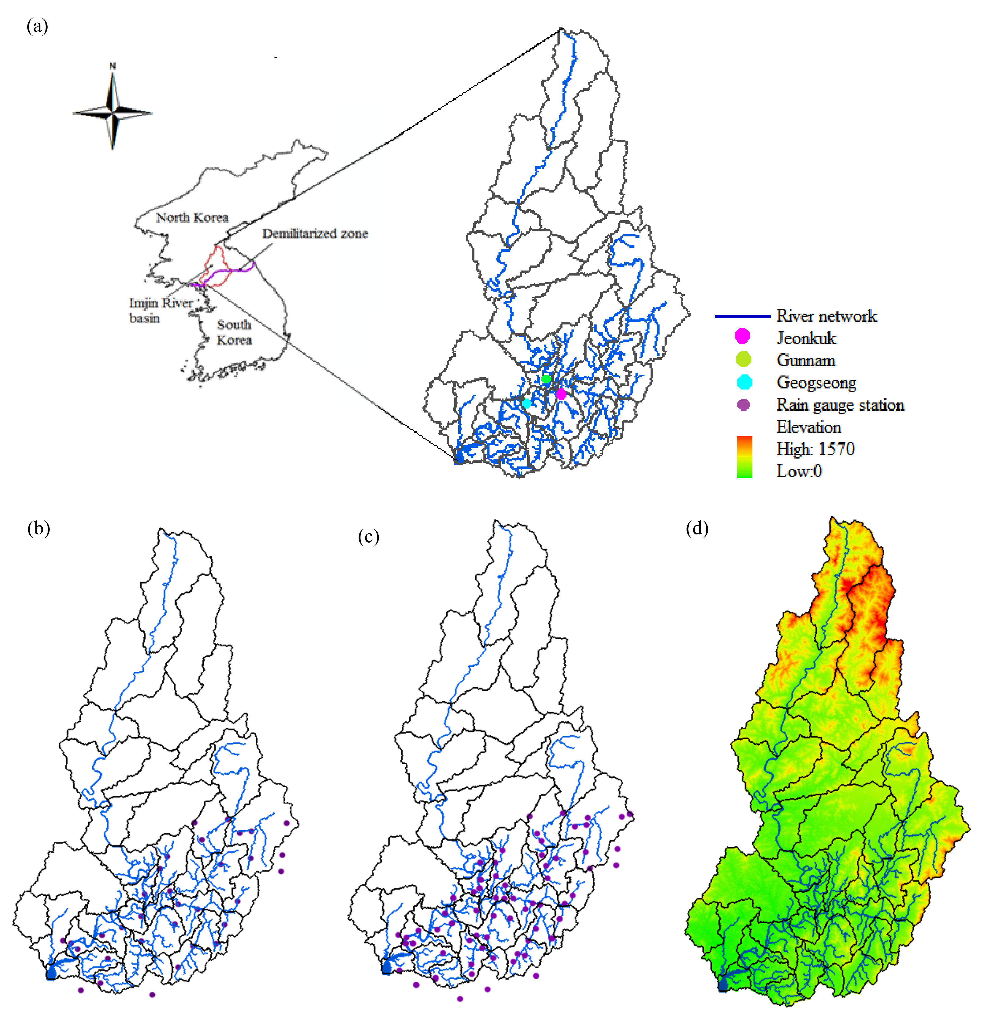
2. Study Area and Data

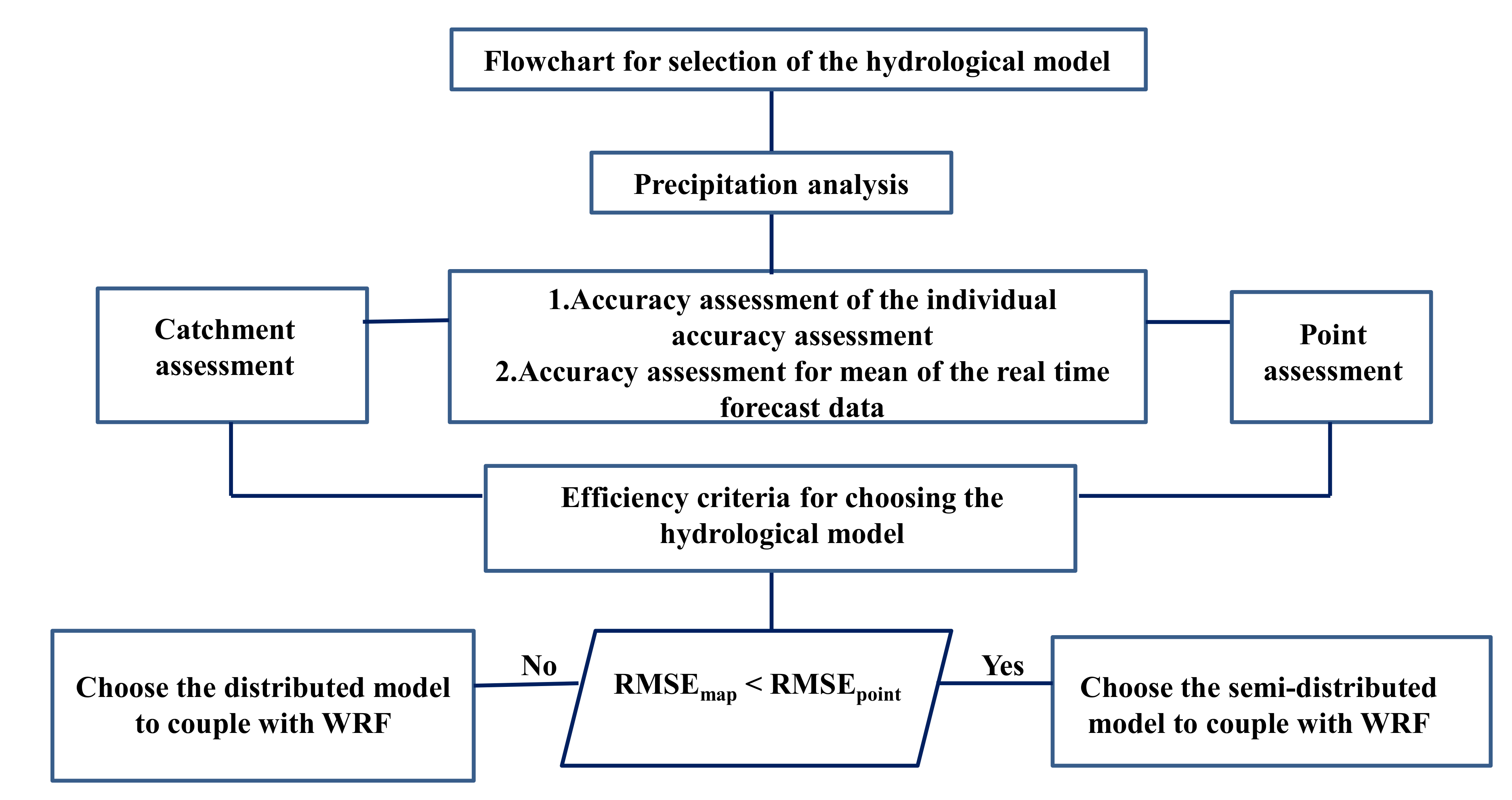
Documents and analysis will entirely focus on the Imjin River, the seventh largest river in the Korean peninsula, which passes through North and South Korea. The area and the length of this domain are 8139 km² and 273.5 km, respectively. The river originates in North Korea, heads from the Hamgyeongnam-do Masikryoung Duryu mountain and flows from North to South passing the demilitarized zone (DMZ), and joins the Han River and finally the Yellow Sea. The average annual precipitation is approximately 1100 mm [23], and the topography varies from 155 m to 1570 m above mean sea level. Since two-thirds of the Imjin River is located in North Korea, this river is considered a transboundary river. Given that immediate access to data in Transboundary Rivers is hard due to political boundaries and data reliability, Transboundary Rivers are always challenging for engineers and model developers. Therefore, it was difficult to obtain the required information for the hydrological model in the northern part of the basin. In addition, the study area includes 38 subbasins. The subbasins and location of water level gauges are shown in Figure 1, which provides a broad depiction of the study area.

Other applications of the flood forecasting system are greatly related to military operations. The coupling of hydrological and meteorological models is done to enhance flood information analysis in this important area. Heavy rainfall and repeated storms have been reported many times in South and North Korea, especially during the summer and fall. The Imjin River has encountered various flood events across several years. The extreme events are chosen for consideration in flood forecasting in the Imjin River basin. The list of the investigated events is shown in

Table 1. List of the investigated events in Imjin basin.

Case Number	Event ID	Event Period
1	2002	28 August–4 September 2002
2	2007	23 July–4 September 2007
3	2011	25 July–30 July 2011

.

In 2002, Typhoon Rusa ripped through South Korea in the Gangneung area between 31 August and 1 September, affecting the eastern and southern parts of Korea with almost 900 mm of rainfall in 30 h [24]. The typhoon caused the submergence of 9000 houses and killed 113 people. In 2007, North Korea had heavy rain between 7–14 August and 18–20 September (caused by Typhoon Wipha). Over seven days, approximately 500–700 mm of rainfall caused this flood in North Korea. Seoul also experienced heavy flooding on 27 July 2011. In the case of fast growing densely populated cities such as Seoul, flash floods of 536 mm of rainfall in three days resulted in 69 people reported as dead or missing in the Gangnam area. Flood events in Imjin basin caused damages to the buildings, agricultural fields, roads, water structures, military equipment and marine facilities. In Imjin basin the number of death is 41, 4 and 37; number of the property damages is 14, 22 and 95 and total financial damages are approximately 3,500,000, 800,000 and 1,400,000$ in the events 2002, 2007 and 2011, respectively [25].

These intense rainfall events led to hazardous floods and caused various damages in South and North Korea. The floods were caused by torrential rainfall in this area and indicate the need for integrated flood management, especially for two countries with different natural environments and national defenses. In the Imjin basin for North Korea, there are more mountains and higher altitudes by comparing with South Korea (Figure 1d). Therefore, the North and South Korea have different natures in the Imjin basin. The differences between North and South Korea for average, maximum and minimum temperature, precipitation and relative humidity are shown in the

Table 2. Meteorological data information for South and North Korea in Imjin basin.

Meteorological Data	South Korea	North Korea
Average temperature (°C)	12.1	8.7
Maximum temperature (°C)	38.4	22.6
Minimum temperature (°C)	−20.2	−16.7
Precipitation (mm)	1361.8	1173.2
Relative humidity (%)	67.5	76.0

. It should be noted that this data are provided by Global Telecommunication System (GTS) for South and North Korea [26].

In this study, the meteo-hydrological components are coupled for real-time rainfall-runoff forecasting procedures for the transboundary Imjin River. There are 66 rain gauges for the events 2007 and 2011 (Figure 1b) and 33 rain gauges for the event 2002 (Figure 1c), and there are three meteorological stations in the Imjin basin. The number of rain gauges is changed after 2002 due to the Gunnam flood control project which started in 2003.The observation data used in this study were passed through a quality control procedure, which checked the values and filled missing values by interpolating from nearby stations to complete the hourly data from all stations.

3. Methodology

3.1. Meteorological Model of Weather Research and Forecasting (WRF)

The WRF model is a mesoscale NWP model designed for atmospheric and operational forecasting research. The WRF includes two dynamical cores, data assimilation and software. The WRF model applies to a wide range of meteorological issues at various scales. The application of the WRF model as a mesoscale model for forecasting extreme events has been used worldwide. This model enables researchers to conduct different atmospheric simulations, such as real data or idealized conditions, by providing operational forecasting, including advances in physics, numeric and data assimilation. The initial and boundary conditions were obtained using external sources, such as the static geographic data provided by the USGS and MODIS data set and the gridded data provided by regional and global models such as the North American Mesoscale Forecast system (NAM) and the Global Forecast System (GFS) [27]. In summary, using the definitions of all computational grids, geogrid interpolates terrestrial, time invariant fields, and then Ungrib extracts the meteorological fields from the GRIdded Binary (GRIB) formatted files, and Metgrib horizontally interpolates the meteorological data to the simulation domains. The Advanced Research WRF (ARW) solver uses time-splitting techniques to integrate the fully compressible non-hydrostatic equations of motion. The Euler equations are in flux form and are formulated using a terrain that follows mass vertical coordinates. Finally, time-split integration is carried out using the second or third order Runge-Kutta method [27].

The parametrization of the precipitation in NWP models is a very important factor. The WRF model contains various microphysics schemes including the cumulus scheme and microphysics scheme. There have been numerous studies of the WRF model in Korea, but the performance of the different WRF schemes in heavy rainfall has not been comprehensibly studied. Among them, two studies evaluated the mentioned schemes in Korea. According to the findings of Hong, the cumulus parameterization scheme based on convective instability is responsible for producing heavy rainfall over the central United States, whereas it plays a less dominant role in the heavy rainfall in the Korean peninsula [28]. According to the study done by [29] for simulating heavy rainfall using WRF model over the Korean peninsula it was found that WDM6 microphysical scheme simulated best the vertical structure of heavy rain [29]. Since our study is focused on the extreme rainfall and flood events, the WDM6 microphysical scheme was chosen for the present study. We did not consider a cumulus scheme. Furthermore, the microphysics scheme of our numerical setup is WDM6. Normally, a cumulus scheme is not consider in the high resolution (1 km) simulation because no cumulus scheme means that cloud was resolved within high resolution grid. Moreover, WDM6 has stable performance in rainfall simulation, although WDM6 tends to underestimate the rainfall. In the present study, the WRF version 3.5.1 was used for real-time forecasting of the meteorological data by using the WRF Double-Moment 6-Class (WDM6) microphysical scheme. The global meteorological reanalysis datasets were used in the study NCEP Final Analysis (FNL; National Centers for Environmental Prediction) for the initial condition (IC) and boundary condition (BC) of the WRF model. The resolution is 1 × 1 degree grids. On the meteorological side, the WRF model covered Korea and the surrounding region with a high temporal and spatial resolution. The WRF model is configured on a Mercator projection with 400 × 400 × 40 grid points and high resolution of 1 km × 1 km.

3.2. Hydrological Model: Sejong University Rainfall Runoff Model (SURR)

To find the proper hydrological model, the assessment of the forecasted precipitation for rain gauge stations and MAP are done using individual forecasts and the mean of the forecast data (Figure 2). The quality of forecast precipitation can be analyzed by comparing the values with observation data. For this purpose, precipitation analysis can be done by the average ensemble method using equal weighting to the members, which are lagged by 6 h.

This approach included forecast averages from multiple lead-times, which were then compared with observed data. The methodology used to compare the observation and with the average of the real-time ensemble forecast data is depicted in Figure 3. The Root Mean Square Error (RMSE) is used for the comparison between real-time forecast data and the observed data. The RMSE is one of the most widely used approaches for verification, and it evaluates the average magnitude of real-time forecast errors. The outcomes from this analysis are provided in the Results section (please refer to Section 4.2), and the findings resulted in the selection of the semi-distributed hydrological model that is described as follows.

The SURR was developed by the Water Resource and GIS Laboratory, Sejong University [30]. The model was developed based on the event-oriented storage function model [31]. The SURR model is a semi-distributed continuous rainfall runoff model that improved the estimation of hydrological components such as potential evapotranspiration, surface flow, lateral flow and groundwater flow using physical foundations. This model was developed to illustrate the complicated and nonlinear relationship between rainfall and runoff in combination with natural components, such as soil moisture condition and land use. The SURR model requires the input data as MAP and Mean Areal Evapotranspiration (MAE) for each of the sub-catchments. The SURR model can be driven by either observed or forecasted precipitation data. The FAO Penman-Monteith method was chosen as the method by which evapotranspiration was estimated from meteorological data. The evapotranspiration is calculated using the FAO Penman-Monteith formula. The FAO PM method is recommended as a standard method for estimating evapotranspiration (ET). The FAO PM method can be expressed as Equation (1):

$$ET=\frac{0.408\Delta \left(R_n-G\right)+\gamma \frac{900}{T+273}{u}_2\left(e_s-e_a\right)}{\Delta +\gamma \left(1+0.34u_2\right)},$$

(1)

where ET is the evapotranspiration [mm day⁻¹], Rn is the net radiation at the crop surface [MJ m⁻² day⁻¹], G is the soil heat flux density, which is relatively small for daily and 10-day periods [MJ m⁻² day⁻¹], T is the mean daily air temperature at a height of 2 m [°C], u2 is the wind speed at a height of 2 m [m s⁻¹], es is the saturation vapor pressure [KPa], ea is the actual vapor pressure [KPa], es-ea is the saturation vapor pressure deficit [KPa], ∆ is the slope vapor pressure curve [KPa °C⁻¹] and γ is the psychrometric constant [KPa °C⁻¹]. The meteorological data are used to calculate the ET and then the Thiessen polygons are used by GIS to estimate the MAE for each sub-basin. The rainfall and evapotranspiration data have hourly temporal resolutions, which were spatially interpolated by the Thiessen polygons method using GIS.

Hydrological model parameters and formulation affect the ability of the hydrological model to simulate the streamflow. Therefore, as an initial assessment, the calibration and verification of the hydrological model could be done using historical data to determine the stability of the model. In the SURR model, there are two types of incorporated parameters, which include the subjective and objective parameters. The subjective parameters can be estimated based on the basin characteristics using GIS while the objective parameters are computed in the model calibration process. The subjective and the objective parameters of the SURR model are presented in

Table 3. The subjective and objective parameters in the Sejong University Rainfall Runoff (SURR) model.

Subjective Parameters	Definition	Unit	Estimation Method
AKM	Subbasin area	km2	GIS
SLP	Mean slope of the subbasin	m/m	GIS
Z	Depth of soil layer	m	GIS
SAT	Rate of water content at saturation	mm/mm	GIS
FC	Rate of water content at field capacity	mm/mm	GIS
WP	Rate of water content at wilting point	mm/mm	GIS
KS	Saturated hydraulic conductivity	mm/h	GIS
CN2	Runoff curve number under AMC II	-	GIS
Objective Parameters
LHILL	Mean slope length	m	Calibration
SURLAG	Surface runoff lag coefficient	h	Calibration
LAGSB	Lag time of the subbasin	h	Calibration
LATLAG	Lateral flow lag coefficient	h	Calibration
SEPLAG	Delay time for water percolating	h	Calibration
GWLAG	Delay time for aquifer recharge	h	Calibration
ALPHA_BF	Baseflow recession constant	-	Calibration
AQMIN	Threshold water level in shallow aquifer for baseflow	mm	Calibration
Ksb	K coefficient of the subbasin	hPsb	Calibration
Psb	P coefficient of the subbasin	-	Calibration
Kch	K coefficient of the channel	sPsb	Calibration
Pch	P coefficient of the channel	-	Calibration

.

For rainfall runoff simulation, the sensitive parameters of the SURR model are P_ch, P_sb, K_sb and K_ch. The calibration and verification events used in this study are provided in

Table 4. The calibration and verification periods for SURR model simulations.

Case Number	Event ID	Event Period
1	Calibration	23 July–3 September 2007
2	Calibration	1 July– 22 August 2008
3	Verification	21 June–4 August 2009
4	Verification	9 July–20 August 2010
5	Verification	16 June–2 August 2011
6	Verification	31 July–13 September 2012

. The SURR model was calibrated for the Imjin basin using the observed rainfall and streamflow, and the optimized parameters resulted in good agreement between the observed and simulated streamflow during the verification periods.

The efficiency criteria used in this study are presented in

Table 5. Statistical measures used to evaluate model performances.

Index	Formula	Range	Ideal Value
Root Mean Square Error (RMSE)	$\mathrm{RMSE}=\sqrt{\frac{{{\displaystyle \sum }}_{\mathrm{i}=1}^{\mathrm{N}}{\left({\mathrm{O}}_{\mathrm{i}}-{\mathrm{S}}_{\mathrm{i}}\right)}^2}{\mathrm{N}}}$	(0,∞)	0
Nash-Sutcliffe Efficiency (NSE)	$\mathrm{NSE}=1-\frac{{{\displaystyle \sum }}_{\mathrm{i}=1}^{\mathrm{N}}{\left({\mathrm{O}}_{\mathrm{i}}-{\mathrm{S}}_{\mathrm{i}}\right)}^2}{{{\displaystyle \sum }}_{\mathrm{i}=1}^{\mathrm{N}}{\left({\mathrm{O}}_{\mathrm{i}}-\overline{\mathrm{O}}\right)}^2}$	(−∞,1)	1
Correlation	$\mathrm{Correlation}=\frac{{{\displaystyle \sum }}_{\mathrm{i}=1}^{\mathrm{N}}\left({\mathrm{O}}_{\mathrm{i}}-\overline{\mathrm{O}}\right)\left({\mathrm{S}}_{\mathrm{i}}-\overline{\mathrm{S}}\right)}{\sqrt{{{\displaystyle \sum }}_{\mathrm{i}=1}^{\mathrm{N}}{\left({\mathrm{O}}_{\mathrm{i}}-\overline{\mathrm{O}}\right)}^2{{\displaystyle \sum }}_{\mathrm{i}=1}^{\mathrm{N}}{\left({\mathrm{S}}_{\mathrm{i}}-\overline{\mathrm{S}}\right)}^2}}$	(−1,1)	1
Relative Error in Volume (REV)	$\mathrm{REV}=\frac{\sum {\mathrm{S}}_{\mathrm{i}}-\sum {\mathrm{O}}_{\mathrm{i}}}{\sum {\mathrm{O}}_{\mathrm{i}}}\times 100$	(−∞,∞)	0
Mean Relative Error (MRE)	$\mathrm{MRE}=\frac{1}{\mathrm{N}}{\displaystyle {\displaystyle \sum }_{\mathrm{i}=1}^{\mathrm{N}}}\frac{{\mathrm{S}}_{\mathrm{i}}-{\mathrm{O}}_{\mathrm{i}}}{{\mathrm{O}}_{\mathrm{i}}}$	(−∞,∞)	0
Bias	$\mathrm{Bias}=\frac{1}{\mathrm{N}}{\displaystyle {\displaystyle \sum }_{\mathrm{i}=1}^{\mathrm{N}}}{\mathrm{O}}_{\mathrm{i}}-{\mathrm{S}}_{\mathrm{i}}$	(0,∞)	0

Note: ${\mathrm{O}}_{\mathrm{i}}$: Observed streamflow; ${\mathrm{S}}_{\mathrm{i}}$: Simulated streamflow; $\overline{\mathrm{O}}$: Average of observed streamflow; $\overline{S}$: Average of simulated streamflow.

. These criteria include the Root Mean Square Error (RMSE), Nash-Sutcliffe Efficiency (NSE) by [32], Correlation and Relative Error in Volume (REV).

The statistical analyses of the SURR model simulations for the calibration and verification events are shown in

Table 6. Statistical analysis of simulated flow for calibration and verification periods in SURR model.

Error Measurement	Calibration Period 23 July–3 September 2007			Calibration Period 1 July–22 August 2008			Verification Period 21 June–4 August 2009
	Gunnam	Jeonkuk	Jeogseong	Gunnam	Jeonkuk	Jeogseong	Gunnam	Jeonkuk	Jeogseong
RMSE	629.36	182.87	864.82	599.13	139.52	609.68	632.18	196.79	766.87
Nash	0.69	0.78	0.71	0.70	0.83	0.79	0.57	0.85	0.79
Correlation	0.85	0.95	0.91	0.82	0.97	0.93	0.84	0.96	0.92
REV	−0.48	−0.12	−0.52	0.37	0.03	0.08	0.16	−0.22	0.03
Error Measurement	Verification Period 9 July–20 August 2010			Verification Period 16 June–2 August 2011			Verification Period 31 July–13 September 2012
	Gunnam	Jeonkuk	Jeogseong	Gunnam	Jeonkuk	Jeogseong	Gunnam	Jeonkuk	Jeogseong
RMSE	702.59	263.35	779.22	621.33	220.18	704.99	688.67	77.19	616.71
Nash	0.62	0.71	0.67	0.71	0.89	0.85	0.59	0.78	0.66
Correlation	0.63	0.92	0.84	0.84	0.97	0.93	0.62	0.95	0.81
REV	0.23	−0.34	−0.07	−0.09	−0.19	−0.11	−0.28	−0.20	−0.05

.

The RMSE, NSE, Correlation and REV are used to compare the simulated and observed stream flow in calibration and verification periods. For the sake of the brevity, the results of the calibration and verification are shown for the 2008 and 2012 events for Jeonkuk station (Figure 4). A detailed description of the SURR model is reported in [30,33].

3.3. Accuracy Assessment

In this research, the results were obtained based on a one-way coupling methodology that connected the SURR and WRF models. To further investigate the accuracy of the coupled meteo-hydrological models, it is essential to use a methodology that quantifies the errors of the coupled system. As mentioned before, this study does not focus on the errors related to the hydrological model performance; therefore, the overall procedure consists of quantifying the accuracy of the precipitation analysis, the spatial and temporal resolution and the variation in lead-time using statistical measures.

The precipitation is the most important output of meteorological models used for meteo-hydrological applications since the performance of coupled meteo-hydrological models is dependent on the accuracy of forecasted precipitation. Therefore, it is necessary to establish a methodology to analyze the real-time forecast data. Point precipitation analysis provided a comparison between the observed precipitation at rain gauge stations and the values that were forecast for each place. Furthermore, the areal average values of precipitation were calculated by Thiesen polygons at the catchment scale using the observed precipitation at the rain gauge stations versus the high resolution of the meteorological model forecast data. The accuracy assessment of variations in spatial resolution (1, 2, 4, 8, 12, 16 and 20 km), temporal resolution (10, 20, 30 and 60 min) and lead-time (12, 24, 36, 48, 60 and 72 h) can be performed by evaluating the precipitation and analyzing the discharge. The correlation, bias and RMSE can be used to show the level of agreement between the observed and forecasted values and the accuracy variation for the abovementioned items, respectively. In this study, we considered each factor separately for example in spatial resolution analysis the temporal resolution of 10 min and forecast lead-time of 72 h are fixed and comparison is done by changing the spatial resolutions. In temporal resolution analysis, the spatial resolution of 1 km × 1 km and forecast lead-time of 72 h were fixed and the evaluations are done for four different temporal resolutions. Accordingly, for the forecast lead-time analysis, the spatial resolution of 1 km × 1 km and temporal resolution of 10 min were fixed and then the evaluations were done for various forecast lead-times.

According to the results of this analysis, the optimal spatial and temporal resolution and lead-time can be chosen to be used in the time series analysis of forecast flood. Evaluation techniques have been reviewed using a variety of gauge and forecasted data in the SURR and coupled SURR-WRF models. With these different types of comparisons, it is possible to establish the quality of each component. Comparisons of simulated, observed and forecast stream flow can be done using statistical indexes to quantify the accuracy assessments. The efficiency criteria used in this study are presented and evaluated (Table 5). These criteria include the NSE, Mean Relative Error (MRE) and REV. These indexes provide more information on the systematic and dynamic errors present in the model results.

4. Results and Analysis

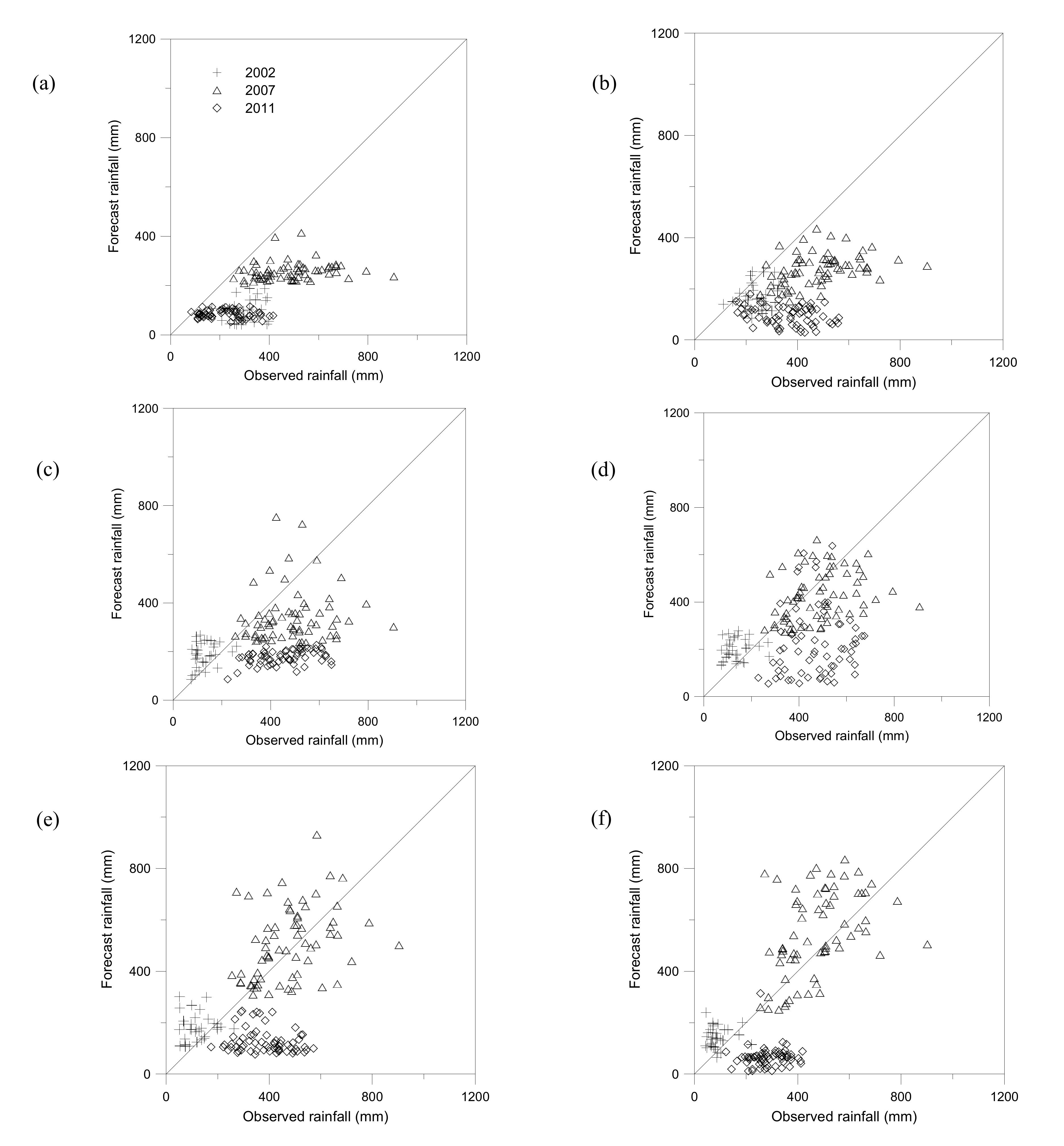
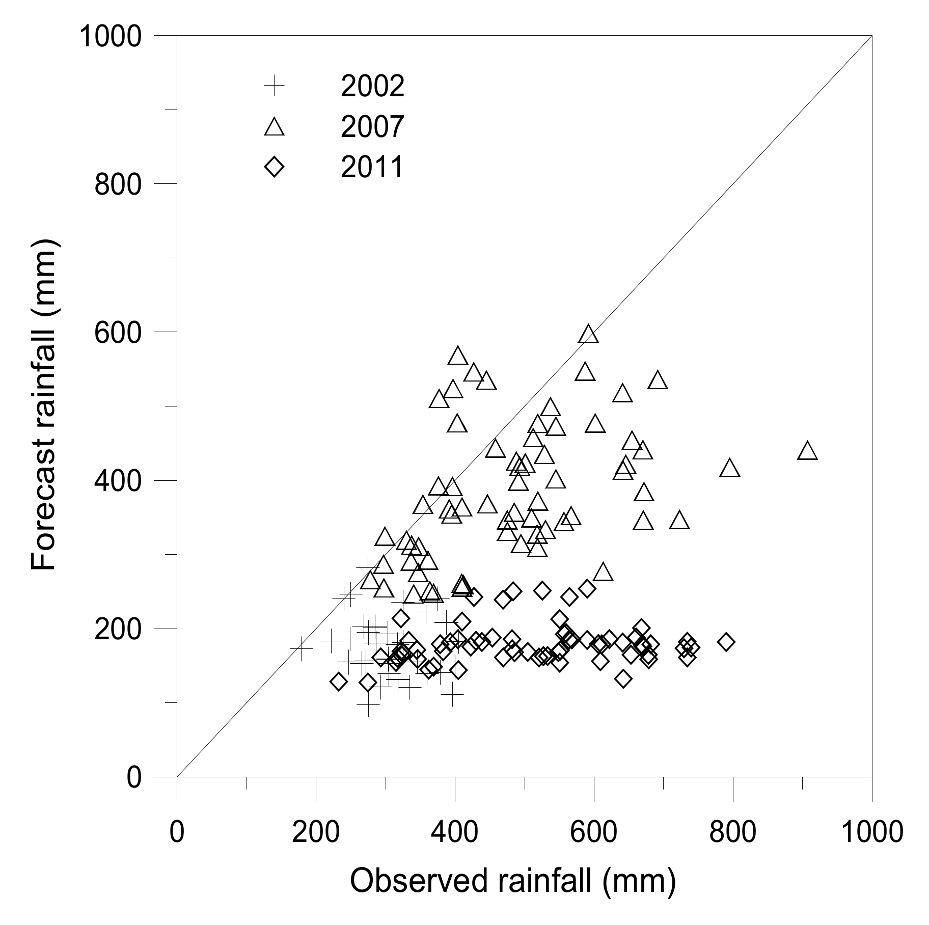
4.1. Point Precipitation Assessment

In coupled meteo-hydrological models, for real-time flood forecasting, the error related to the rainfall forecasts overcomes the other sources of error. In this part, the attention is focused solely on the meteorological model. Observed precipitation has a complicated nature, which makes it difficult to use for atmospheric validation, but it could be a useful tool for detecting precipitation errors, such as those caused by the position, timing and strength of the events. The amount of precipitation produced by the atmospheric model is compared with rain gauges to diagnose the forecast errors. Due to the high resolution of the WRF model in this study, the error related to locating different stations in the same model grid cell with different observations is eliminated. This analysis is applied for spot measured rainfall in observation stations and for real-time forecasted data from the WRF model at the mentioned locations.

In this method, each observation is compared with a single corresponding mean forecast data from the same time. Precipitation analysis at the point scale shows that the skill of the NWP precipitation forecasts varies considerably between rain gauge stations. The results of the point precipitation assessment at the 33 stations for the 2002 event and the 66 stations for the 2007 and 2011 events indicated that the WRF model does not forecast the rainfall well. Further investigation is conducted to compare the total, minimum, maximum and underestimation of observed and forecast rainfall for the duration of the events (

Table 7. Statistics of point precipitation analysis.

Events	2002		2007		2011
	Observation	WRF	Observation	WRF	Observation	WRF
∑ (mm)	10125	5813	32129	25446	33516	11818
Min (mm)	179	98	278	247	233	127
Max (mm)	405	282	907	599	790	253
Underestimation (%)	94.0		84.8		100

).

The scatter plot of observed and forecast precipitation showed that the WRF model less accurately captures the precipitation accurately in all events. In the present study, the WRF as a NWP model has the limitation of underestimating the precipitation in this study area (Figure 5).

The comparison of the accumulated rainfall in each station is drawn to indicate the variation of the observed and forecast rainfall in all events (Figure 6).

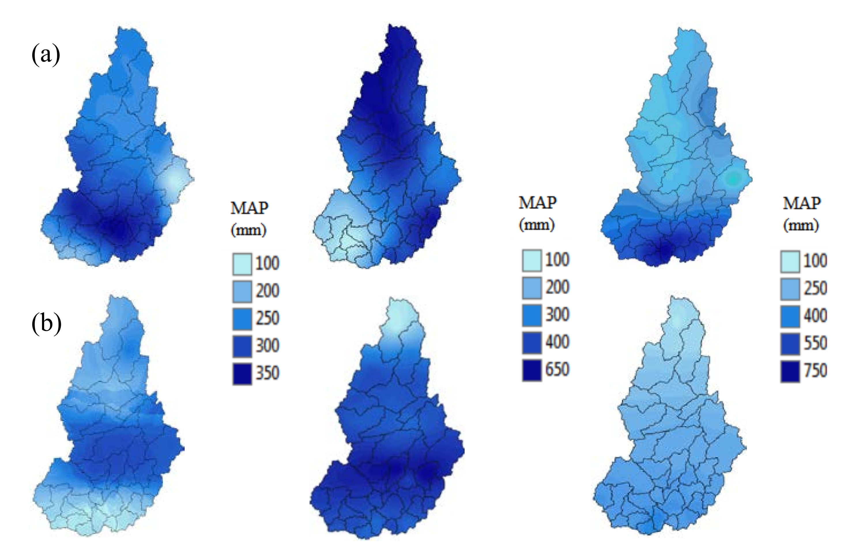
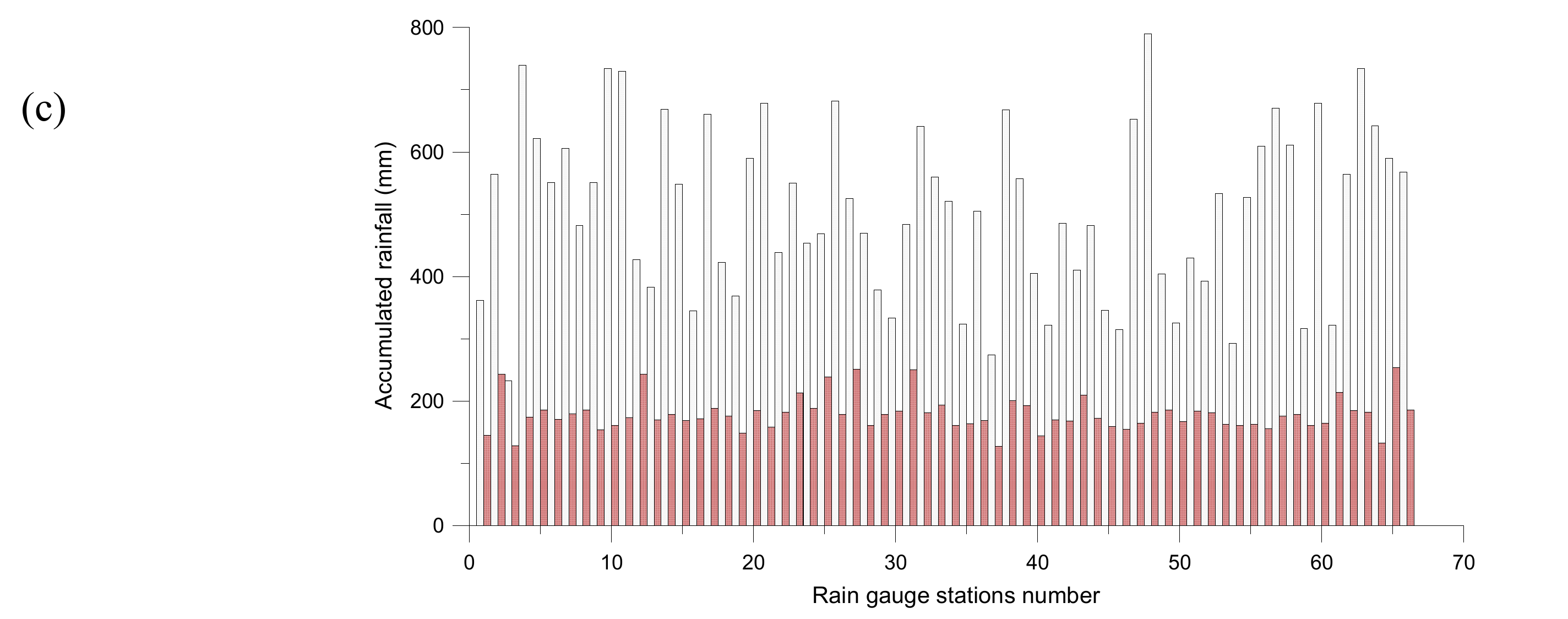
4.2. Spatial Distribution of MAP

To have a general view of the meteorological models’ performance, it is of great necessity to evaluate the NWP model performance at the catchment scale. The figures demonstrate the spatial patterns of MAP, which were obtained by the observed and forecasted precipitation for each subbasin in the Imjin watershed. The observation-based MAPs were calculated using observed precipitation, while the forecast MAPs were obtained from the WRF model. The differences can be detected in the intensities of the observed data and the WRF model data in the whole area. In the flood event of 2002, there is an increasing pattern in the observed data in most of the southern region; however, the WRF model results indicated a decreasing N-S gradient and an increasing pattern in the center region. The results related to the 2007 event showed a positive northbound and southbound gradient of areal precipitation in the observed and forecasted data, respectively. In the 2011 event, the observed and WRF data had an increasing pattern of rainfall from North to South while the WRF results included an underestimation for the MAP. Taken together, at the catchment scale, the WRF model predicted the general rainfall pattern well; however, it had some significant underestimation with respect to the observations (Figure 7).

The results of the MAP assessment showed that the WRF model had underestimated the MAPs by 84.2, 78.9 and 97.4% for the 2002, 2007 and 2011 events, respectively (

Table 8. Statistics of MAP analysis for 38 subbasins.

Events	2002		2007		2011
	Observation	WRF	Observation	WRF	Observation	WRF
∑ (mm)	11100	6796	19041	14623	17445	6710
Min (mm)	197	133	299	159	293	53
Max (mm)	351	264	642	450	743	219
Underestimation (%)	97.37		78.9		100

).

The results of MAP analysis for 38 subbasins exhibited that the WRF model had better performance for the 2002 event, with a lower RMSE of 122 than the higher RMSE of 159 and 304 for the 2007 and 2011 events, respectively (

Table 9. Precipitation assessment for individual and mean forecast real-time data.

Forecast Data	Precipitation Analysis	Error Measurement	2002	2007	2011
Individual forecast	Point assessment	RMSE	84.49	212.80	91.53
	MAP assessment	RMSE	59.67	160.48	68.49
	-	Error reduction (%)	29.38	24.59	25.17
Mean forecast	Point assessment	RMSE	150.42	169.52	355.39
	MAP assessment	RMSE	121.67	158.80	303.58
	-	Error reduction (%)	19.11	6.32	14.59

). Overall, the spatial averaging of rainfall over the catchment reduces the errors compared to point analysis. The accuracy assessment for the comparison of forecast precipitation and MAP indicated that significant differences can be expected for distributed and semi-distributed hydrological models. According to the findings, the semi-distributed hydrological model may be a better choice for this study. For the SURR model, as a semi-distributed hydrological model used in this study, better forecast stream flow can be expected as a result of the lower RMSE in MAP than that from the point precipitation accuracy assessment.

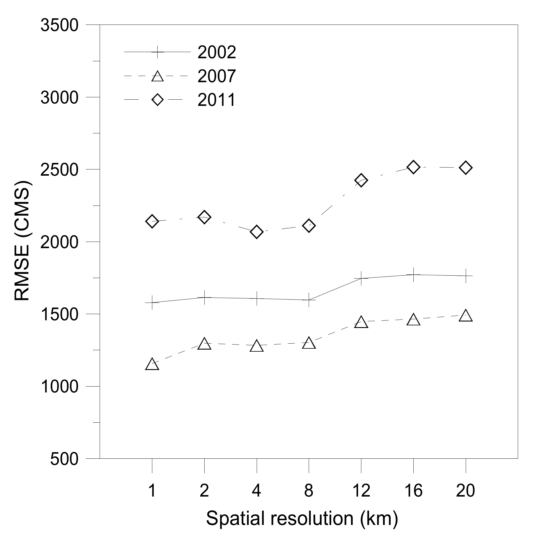
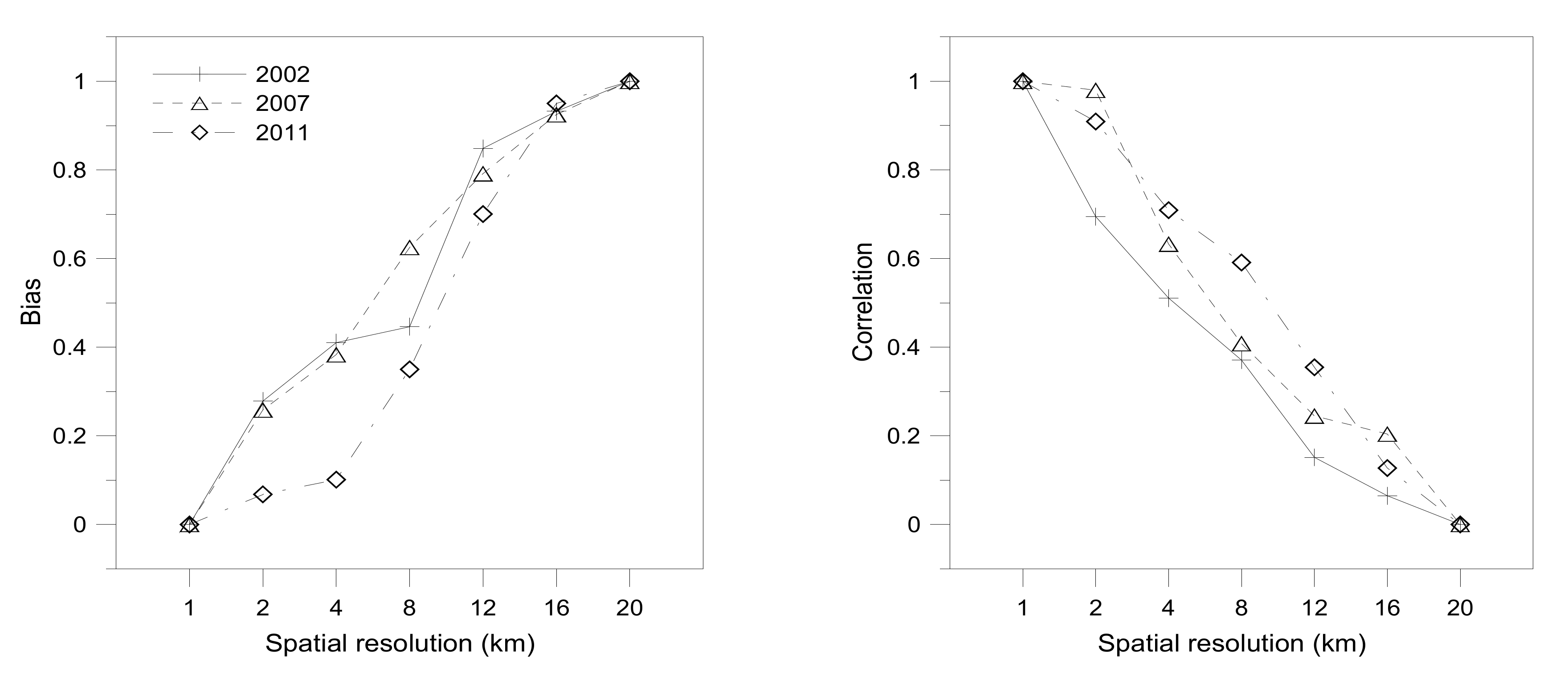
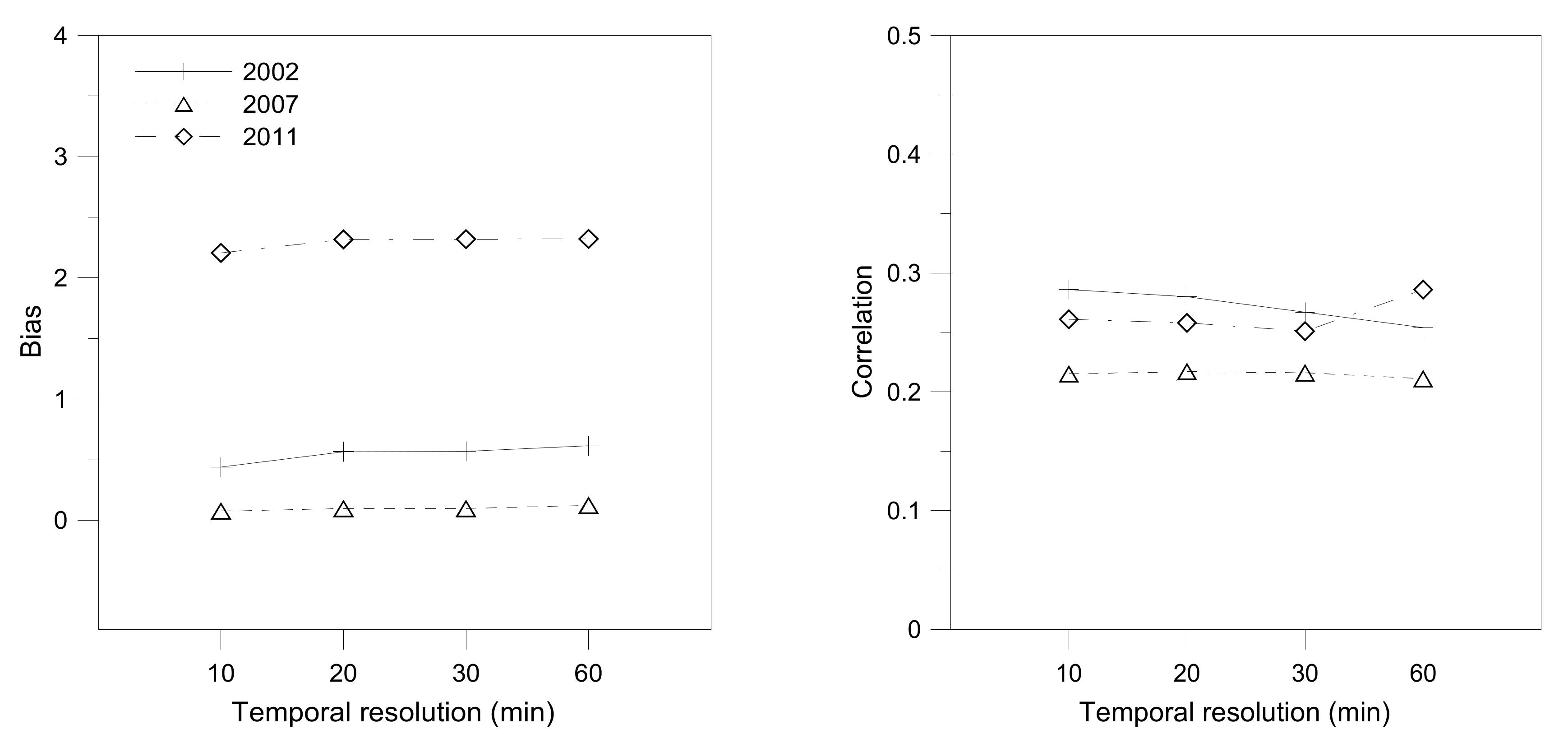
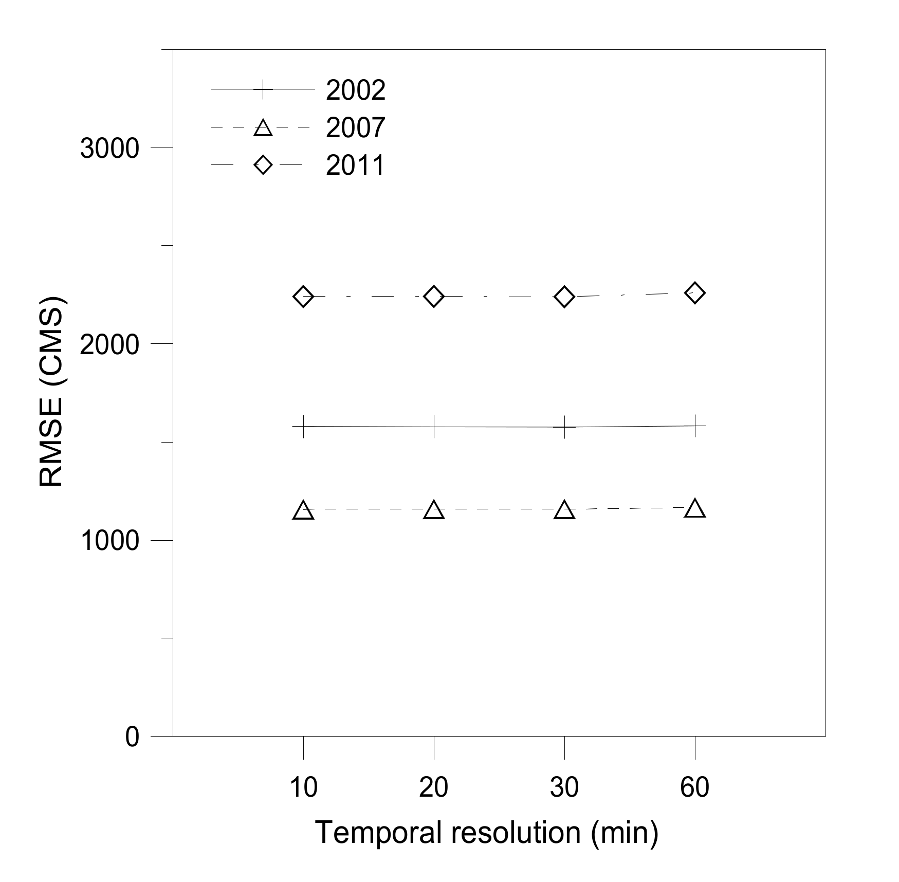
4.3. Spatial Resolution Assessment

It is necessary to assess the spatial resolution effect on the accuracy of coupling the WRF model with the SURR model. Theoretically, higher resolution modeling with better mathematical characterization of physical processes is expected to lead to more accurate forecasts. The WRF model feeds the whole domain of study with a dense spatial resolution. By comparing the spatial resolutions in this study, the results implied that the hypothesis stating higher spatial resolution data have better accuracy is demonstrated by the clear trend of the increasing error percentage with the decreasing spatial resolution in the WRF model. The presentation of the results starts with the evaluation of MAP correlation, the bias of observed and forecast data and the RMSE of streamflow analysis. The recommended minimum spatial resolution is a factor related to the complexity of the study area. The complex terrain and mountainous areas require higher resolutions. The MAP correlation and bias between observed and forecast data are illustrated in Figure 8.

The bias evaluates the difference between the mean of the forecast and observation data, and the correlation illustrates the linear relation among the forecast and observation data. The results indicated that, by decreasing the spatial resolution, the bias increased, and the correlation coefficient decreased for all events. Further analysis led to evaluate the effect of the variation in spatial resolution on the real-time flood forecasting to choose the optimal resolution for coupling the WRF model with the SURR model. To examine the effects of spatial resolution variation on streamflow, the observed and forecasted flows are compared for different spatial resolutions. Increasing the spatial resolution of the meteorological models yielded improvements in the forecasted streamflow (Figure 9). It is determined that the spatial resolutions lower than 8 km did not affect the inherent inaccuracy of the flood forecasts in all events, while after that, the error increased to a higher level for all events. It can be concluded that the WRF model is more likely to resolve physical procedures at higher spatial resolutions.

4.4. Temporal Resolution Assessment

The comparison of variations in temporal resolution of the WRF model forecast with observations for MAP correlation, bias and discharge analysis are indicated in Figure 10 and Figure 11. In addition, as is seen, the accuracy assessment of temporal resolution showed that the performance did not change much by increasing the temporal resolution. The accuracy assessment is implemented to check the temporal resolution variation for 10, 20, 30 and 60 min data.

The results of the bias evaluation for the MAP indicated that the bias did not change significantly for the different temporal resolutions. However, for the 2011 event, the bias is higher than the other events, and this could be related to the underestimation by the WRF model. The results of the MAP assessment in the previous sections (Table 8) showed underestimations of 97.4%, 84.2% and 78.9% for the 2011, 2002 and 2007 events, respectively. The results of the MAP correlation assessment showed that the correlation did not vary significantly for the three events. The findings of the RMSE assessment for flood forecasting illustrated that the temporal resolution variation did not affect the RMSE significantly. Generally, results of MAP correlation and bias, along with error measurement of forecast discharge by RMSE, did not vary for different temporal resolutions in all events.

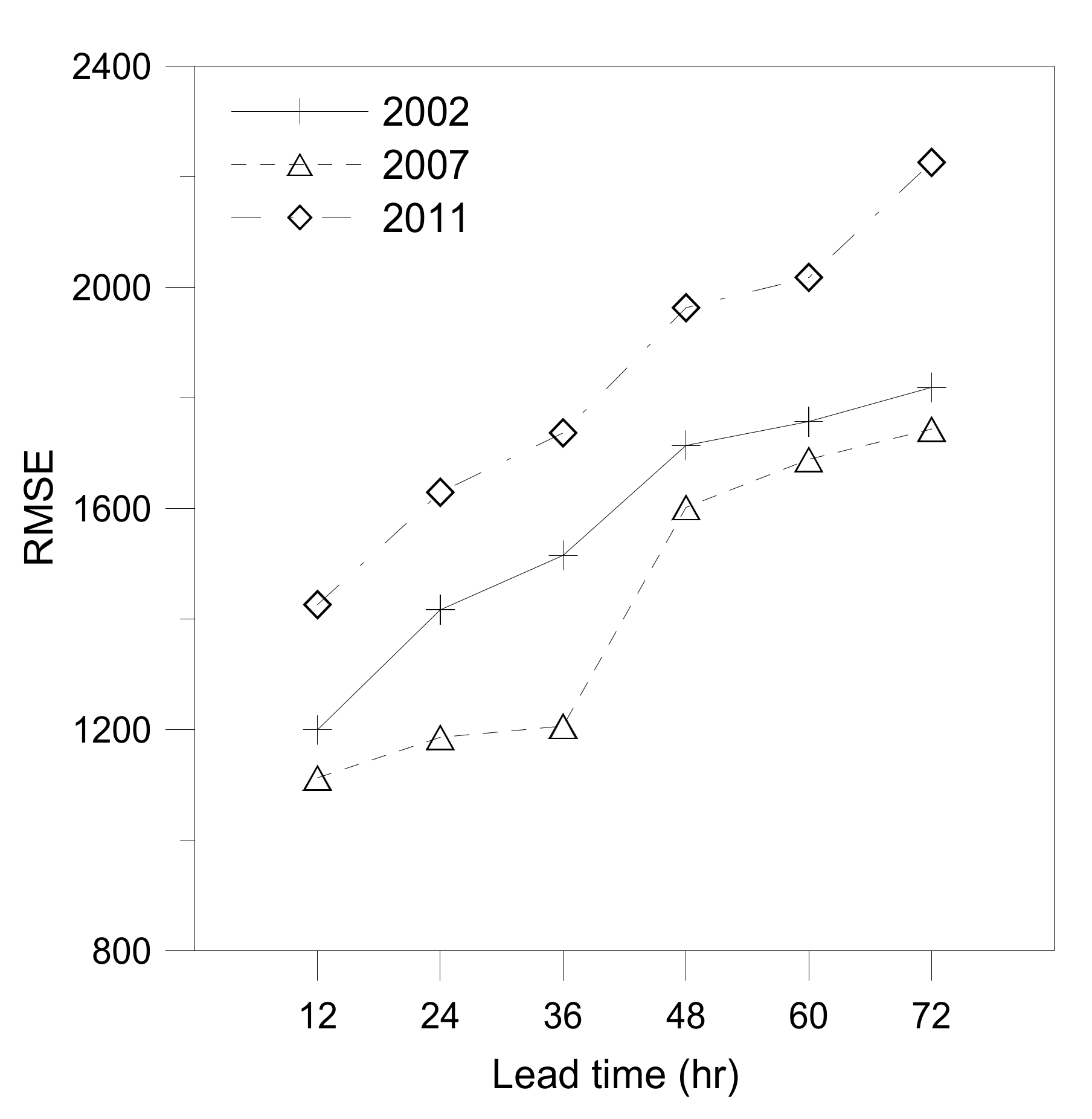
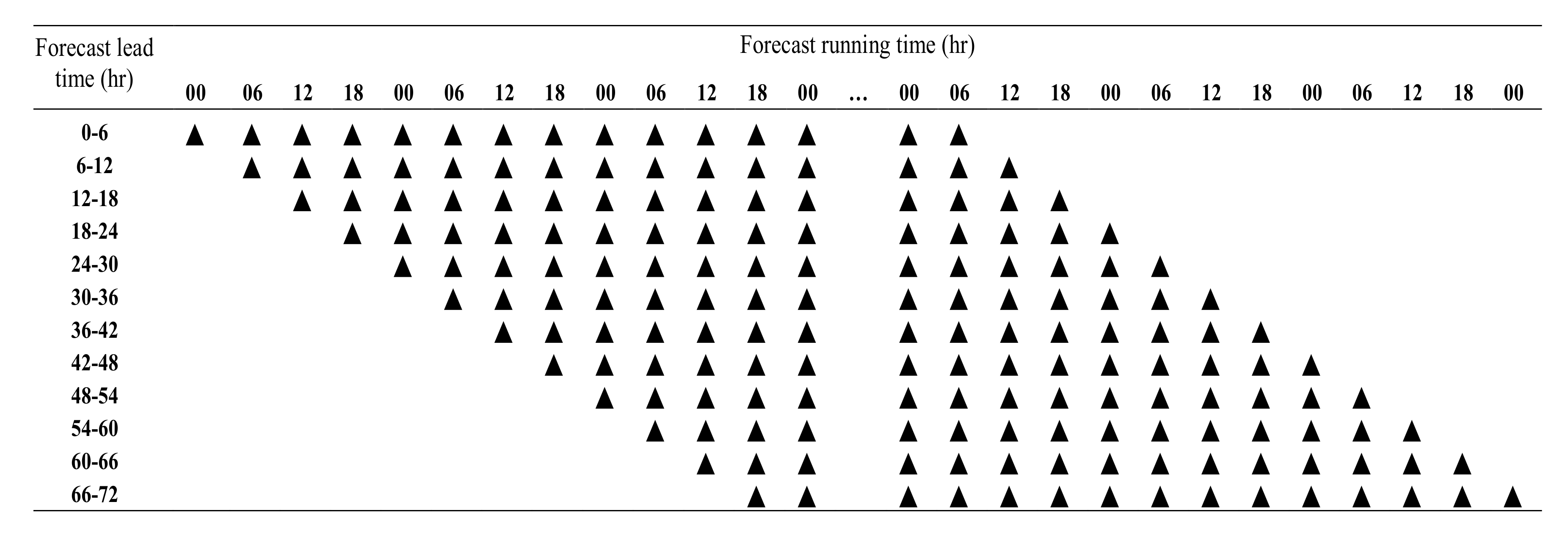
4.5. Lead-Time Variation Assessment

Lead-time is a key factor in the NWP model forecasts since the skills of the models vary significantly with the forecast lead-time. In general, the forecast skill decreases with the increase in lead-time, which is related to higher uncertainty in forecast data. In fact, the NWP models underpin many statistical and hybrid techniques and typically use global-scale models to provide boundary conditions. Accordingly, NWP models are influenced by spin-up effect, which results in deficiencies during the first few hours of the forecast lead-times. The error measurement of each lead-time (L) is given by Equation (2):

$$RMS{E}_L=\sqrt{\frac{1}{N}\sum {\left(Q_{t+L}-{\widehat{Q}}_{t+L}\right)}^2}, L=12,24,36,48,60,72 \mathrm{h}$$

(2)

where N is the number of discharges, ${\widehat{Q}}_t$is the forecasted discharge at time t obtained by the coupled SURR and WRF model, $Q_t$ is the observed streamflow, and L is the lead-time. The summations are for all forecasts, which are the forecast time t belonging to all events. Further analysis compared the performance of the WRF model and the coupled SURR-WRF models with different lead-times. The results showed that the error measurements deviated with changes in lead-time. The accuracy of the model results depended on the forecast lead-time. This indicated that real-time forecasting systems performed better with short forecast lead-times than with longer ones. The results of the observed and forecast rainfall comparison using a scatterplot indicated the over- and underestimation of the forecast rainfall for different lead-time intervals (Figure 12).

The ensemble forecasts of the WRF model results had higher correlation and lower bias for lead-times less than 36 h (

Table 10. The relative bias and correlation assessments for different lead times.

Lead Time (hr)	Event 2002		Event 2007		Event 2011
	Relative Bias	Correlation	Relative Bias	Correlation	Relative Bias	Correlation
0–12	65.00	0.11	32.00	0.17	54.00	0.04
13–24	34.00	0.16	22.00	0.42	52.00	0.27
25–36	60.00	0.20	27.00	0.37	59.00	0.38
37–48	67.00	0.15	33.00	0.35	61.00	0.18
49–60	76.00	0.12	40.00	0.30	64.00	0.17
61–72	93.00	0.03	43.00	0.11	78.00	0.09

).

The discharge error measurement indicated that longer lead-times had lower accuracy as indicated by the increasing RMSE values. Accuracy assessments of lead-time variation demonstrated that lead-time dependency was almost negligible below the 36 h lead-time in the 2002, 2011 and 2007 events (Figure 13).

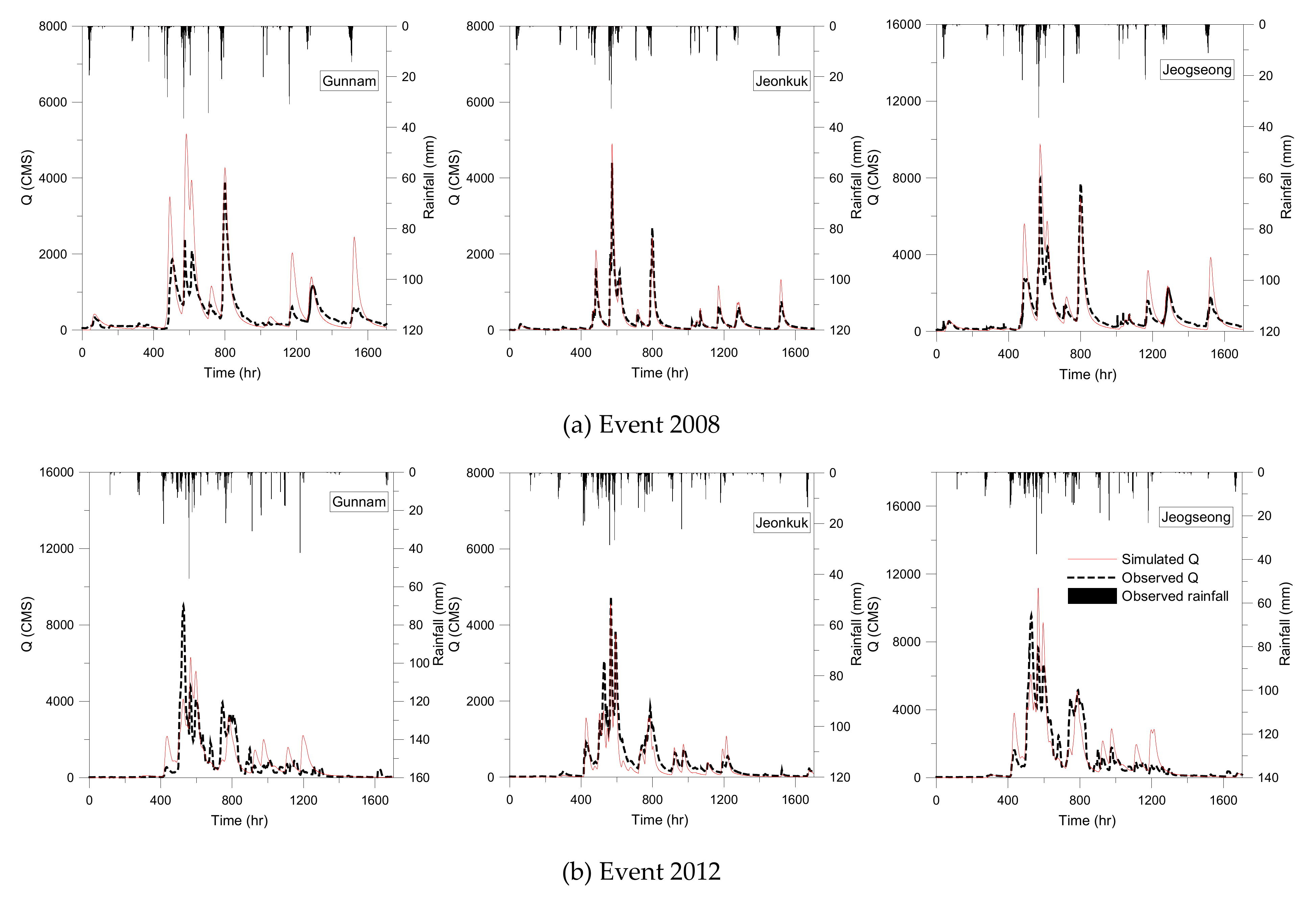
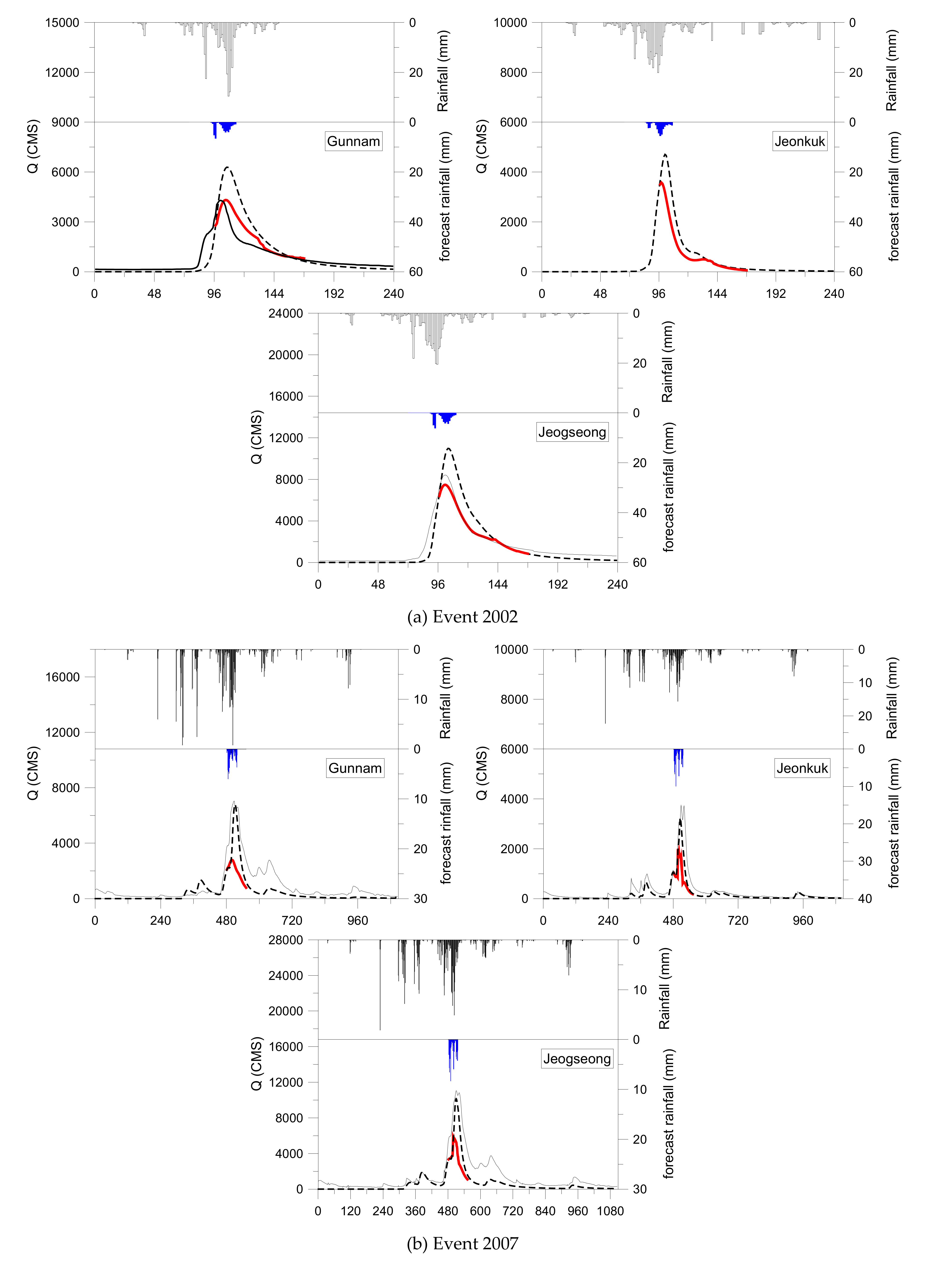
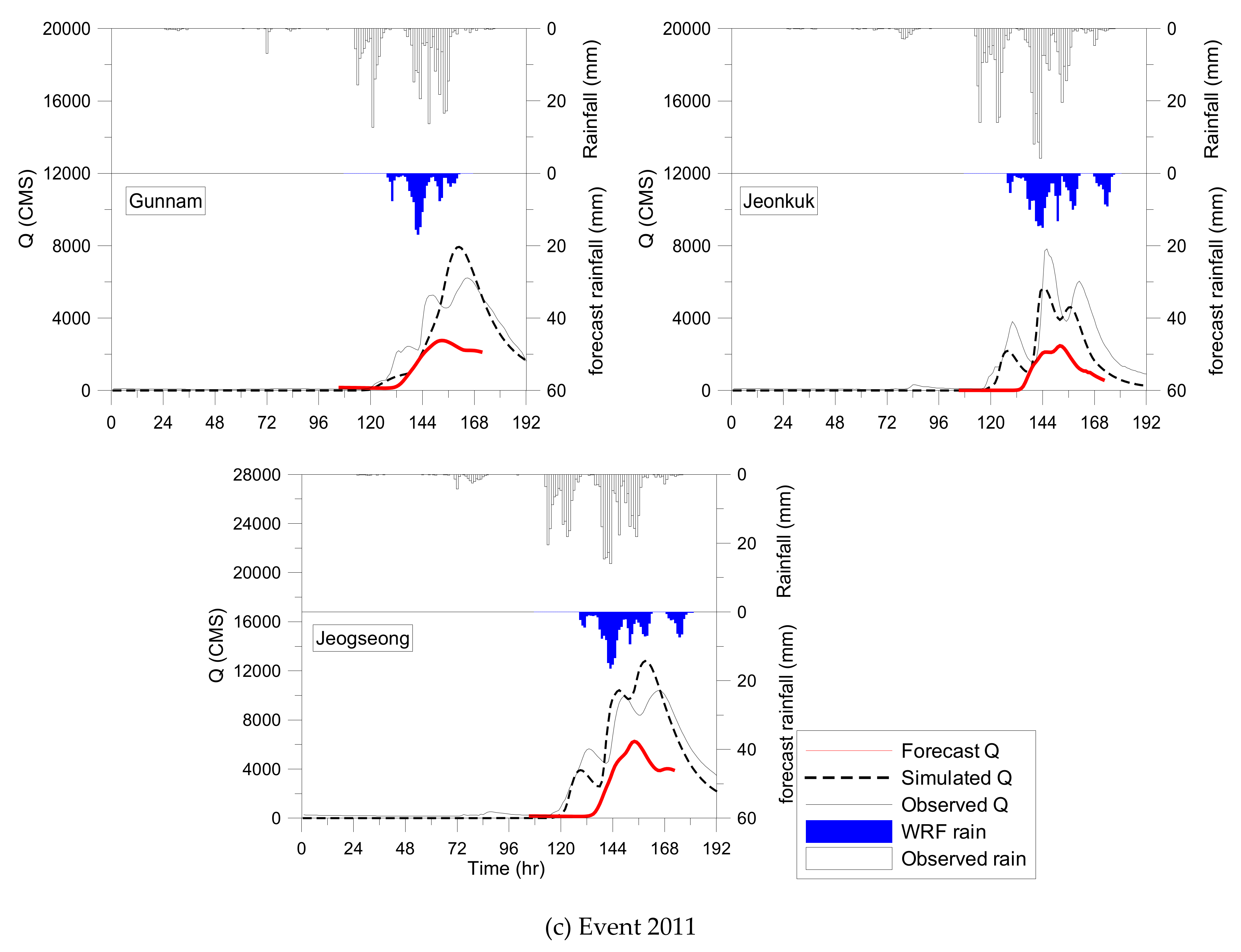
4.6. Time Series Analysis

As previously described, a spatial resolution of 8 km, a temporal resolution of 60 min and a lead-time of 36 h were chosen for coupling the SURR and WRF models in the Imjin basin. Therefore, the time series analysis and the plots of forecast streamflow were created for the abovementioned spatial resolutions, temporal resolutions and lead-times. The accuracy of a streamflow forecast system is dependent upon how well the coupled models are able to make precise results. Consequently, to refuse or agree with the qualification of the model results is vital to establish accuracy measurements. The accuracy of a prediction is evaluated by comparing the observed, simulated and forecasted values. The simulation estimates conducted with the observation MAP and MAE are illustrated as the SURR model input; however, the forecast obtained with the ultra-fine scale, real-time meteorological data from the WRF model are used as the input to drive the SURR model. For the accuracy assessment of the coupled system, statistical error measures are used to describe the average deviations and compare the skill of hydrologic simulations and forecasts produced from the different inputs with observed streamflow. There are some efficiency criteria, such as NSE, MRE and REV, that are frequently used in hydrologic modeling assessments. The Jeonkok has no observation data for the 2002 event. The results of error measurements for the 2002, 2007 and 2011 events illustrated that the coupling system of the two models caused a decrease in the NSE and an increase in the error measurement indexes before and after linking the models (

Table 11. Results of statistical error measurements in Imjin basin.

Index	Gunnam Station		Jeonkok Station		Jeogseong Station
	SURR	SURR-WRF	SURR	SURR-WRF	SURR	SURR-WRF
Event 2002
NSE	0.26	−18.00	-	-	0.68	−19.84
MRE	−0.09	−0.95	-	-	−0.25	0.80
REV	0.16	0.70	-	-	0.03	0.53
Index	Gunnam Station		Jeonkok Station		Jeogseong Station
	SURR	SURR-WRF	SURR	SURR-WRF	SURR	SURR-WRF
Event 2007
NSE	0.69	−4.57	0.78	−6.63	0.71	−10.00
MRE	−0.58	−0.60	−0.06	−0.77	−0.69	−0.78
REV	−0.48	−0.57	−0.12	−0.22	−0.52	−0.54
Event 2011
NSE	0.80	−0.47	0.81	−0.87	0.90	−1.06
MRE	−0.49	−0.79	−0.63	−0.67	−0.06	−0.56
REV	−0.08	−0.59	−0.34	−0.73	−0.45	−0.60

).

Within the NSE range set between 1 (i.e., the ideal value) and negative infinity, values lower than zero indicate that the mean value of the observed streamflow could have better estimate than the model provides. According to the calibration and verification of the SURR model, the results of the streamflow simulations are reasonable and stable with NSEs close to 1; however, for the coupled SURR-WRF model, the NSE decreased dramatically. Here, it should be noted that the calibration of the SURR model parameters is done based on the rain gauge data and observed streamflow, while for real-time flood forecasting by the SURR-WRF coupled system, the real-time precipitation is forecasted using the WRF model. Therefore, the significant differences in NSE and the increases in the error measurement indexes for the SURR and coupled SURR-WRF models are related to the various sources of precipitation used as inputs for the hydrological model.

The performances of the SURR model in simulating the streamflow along with the SURR-WRF coupled model in forecasting the streamflow at the Gunnam, Jeonkok and Jeogseong stations in the 2002, 2007 and 2011 events are presented in Figure 14. The observed stream flow (black curve) is drawn to show the SURR model verification. The red curve indicates the forecast stream flow in the coupled SURR-WRF model, while the solid black curve shows the simulated streamflow using the observed meteorological data. The coupled SURR-WRF model is composed of the observed precipitation until the onset of the forecast time, and it continues using the WRF data to a 36 h forecast lead-time. The combinations of observed and real-time WRF data are used to drive the hydrological model. The observed and real-time forecast precipitations are shown separately in the upper and lower panels of Figure 14, respectively. This procedure is repeated for the next 6 hours to the end of the forecast time. Due to space limitation, briefly, one stream flow forecast is shown with relevant precipitation to indicate the real-time forecast discharge variation over time.

Interestingly, considering the runoff, the amplitudes of the simulated and observed peaks are quite similar in the SURR model simulation, while the amplitudes forecasted by the WRF model are different. This can be explained as the result of the two sources of precipitation, which are basically different. The spatial and temporal variation in the rainfall characteristics were not captured well by the WRF model in the real-time forecast data. In general, it is shown that the NWP models forecast less intermittent precipitation than indicated by the observed precipitation rates. Due to the precipitation parameterization, most of the schemes used in the NWP models have deviations in the forecasted runoff hydrographs with respect to timing and amplitude compared to the measured runoff. Typically, the forecast floods underestimated the peak floods, and the forecasted flood errors are related to the inaccuracies in the real-time forecasted rainfall. Considering all real-time forecast cases from the start of the forecasting time until the end of the forecasting time, on average, it can be concluded that hydrological forecasts based on meteorological model inputs were able to reproduce the shape and the timing of the calculated stream flow fairly well. However, the underestimation of the WRF model precipitation was noticeably affected by the real-time forecast discharge in all events.

5. Discussion

The combination of the NWP models and the hydrological models to generate the flood forecasting is a great topic to study in water related studies. According to the recent studies on coupled meteo-hydrological models, it is necessary to diagnose and evaluate models to more robustly clarify where the models have weaknesses and need improvement. In meteo-hydrological studies, the choosing of the proper hydrological model for coupling with the meteorological model is still an open question. Assessment of the hydrological model selection can be done based on the accuracy of the meteorological model forecast in point and catchment scale. Evaluation of point precipitation and the Mean Areal Precipitation (MAP) could lead to robust decision making in the distributed (which uses the point precipitation data as input) and semi-distributed (which uses the MAP as input) hydrological models. The first objective of this study is to find proper hydrological model to couple with a meteorological model. In order to find the proper hydrological model, the assessment of the forecasted precipitation for rain gauge stations and MAP are done using individual forecasts and the mean of the forecast data.

There are many factors effected the accuracy of the precipitation forecast such as NWP model parametrization, schemes, spin-up time, spatial and temporal resolutions and forecast lead-time. In meteo-hydrological studies, it is clear that the variations in spatial and temporal resolutions as well as in the lead-time of the precipitation forecasts lead to notable differences in the accuracy of flood forecasting. However, it is not yet clarified at which spatial and temporal resolution and lead-time the runoff is forecasted with rational accuracy. In this study, many analyses have been carried out to assess the ability of meteorological and hydrological models to provide hydrological predictions through the estimation of the errors associated with each model. The aim of the present study was to compare the different factors related to the coupling of rainfall runoff forecasting and meteorological systems; additionally, a real-time case study was used to quantify the accuracy assessment of each component. The results of real-time coupled SURR and WRF models highlighted the relative strengths and limitations of the models. The system accuracy assessment was composed of meteorological and hydrological model efficiency.

The results of point precipitation analysis and the spatial distribution of MAP generally indicated that the WRF model produced less accurate precipitation than the observed precipitation rates. The WRF model with high spatial resolution eliminated the error related to locating different stations in the same model grid cell with different observations. The point precipitation analysis showed that the skill of the WRF model varied considerably between rain gauge stations. This might be related to the precipitation parameterization schemes used in the WRF model. The catchment-scale assessment of the WRF model performance by MAP demonstrated the WRF model underestimated the MAP for the events. The hydrological model used in this study benefitted from lower RMSE values in MAP than in point precipitation.

The hypothesis that higher spatial and temporal resolution data have better accuracy is supported in this study; however, based on the findings, the temporal resolution did not have much of a negative effect on the inherent inaccuracy of the data. In general, the results indicated that the real-time forecasting system performed better with short forecasting lead-times than longer ones. During this time, the effects of the initial conditions, spin up, regional characteristics and warm-up time were removed; thus, the results became more reliable. The coupled model performance for all events resulted in runoff peaks of coupled results in cases where time and height were in agreement; however, there was not a good fit with the simulated peaks compared to the observations. The results of the accuracy assessments indicated a decrease in NSE and an increase in error measurement indexes after linking the models. Although the results of the coupled SURR-WRF models have underestimation, available forecast data, especially in a transboundary river such as the Imjin basin, are preferred over completely ignoring future events of interest.

Providing valuable information for flood forecast using the NWP models as the sources of the rainfall forecast and coupling with the hydrological models, can be considered as the credibility of the coupled meteo-hydrological models. The information provided by these kinds of models such as flood forecasting, can be of great importance for water resources managements, providing early warnings to reduce the flood damages. On the other hand, the restrictions of the coupled meteo-hydrological models can be linked to the uncertainties in flood forecasting. For the flood forecasting in meteo-hydrological studies each model component has its own source of producing errors spread from the atmospheric conditions to rainfall forecasts and the rainfall to runoff predictions. The results of the NWP models forecasts have uncertainties and contain biases. Moreover, the uncertainties in flood forecasting could be related to the fact that the hydrological model calibration is done with rain gauge data and observed streamflow; however, the coupled meteo-hydrological model uses the forecast rainfall as the input data to run the model. These are different sources of rainfall were used as input for the hydrological models. Therefore, it could be expected that the hydrological response in forecasting the streamflow would not match the simulated streamflow very well.

6. Conclusions and Recommendations

The main conclusions of this study are listed below:

• The WRF model underestimated the precipitation in this study area in the point and catchment assessments.
• Comparing the results of the point and catchment scale indicated that the WRF model had better performance for the catchment-scale assessment. These findings led to the selection of the semi-distributed hydrological model.
• It was determined that spatial resolutions lower than 8 km did not affect the inherent inaccuracy of the flood forecasts in all events.
• The findings of the RMSE assessment for flood forecasting illustrated that variations in temporal resolution did not affect the RMSE significantly.
• The skill of the WRF model’s real-time forecasts varied significantly with forecast lead-time. Lead-time variation demonstrated that lead-time dependency was almost negligible below 36 h.
• In addition, the QPF is the most important factor driving the hydrological models in coupled studies; therefore, improvements that focus on the QPF post-processing are proposed. Since the lead-time of forecasting is an important factor in real-time flood forecasting, future studies should also focus on potentially improving the lead-time of flood forecasting.

References

1. Chen, X.; Ye, C.; Zhang, J.; Xu, C.; Zhang, L.; Tang, Y. Selection of an Optimal Distribution Curve for Non-Stationary Flood Series. Atmosphere 2019, 10, 31. [Google Scholar] [CrossRef] [Green Version]
2. Wang, Y.; Liu, R.; Guo, L.; Tian, J.; Zhang, X.; Ding, L.; Wang, C.; Shang, Y. Forecasting and providing warnings of flash floods for ungauged mountainous areas based on a distributed hydrological model. Water 2017, 9, 776. [Google Scholar] [CrossRef] [Green Version]
3. Chen, J.; Zhong, P.-A.; Wang, M.-L.; Zhu, F.-L.; Wan, X.-Y.; Zhang, Y. A risk-based model for real-time flood control operation of a cascade reservoir system under emergency conditions. Water 2018, 10, 167. [Google Scholar] [CrossRef] [Green Version]
4. Todini, E. Hydrological catchment modelling: Past, present and future. Hydrol. Earth Syst. Sci. 2007, 11, 468–482. [Google Scholar] [CrossRef] [Green Version]
5. Moulin, L.; Gaume, E.; Obled, C. Uncertainties on mean areal precipitation: Assessment and impact on streamflow simulations. Hydrol. Earth Syst. Sci. 2009, 13, 99–114. [Google Scholar] [CrossRef] [Green Version]
6. Bárdossy, A.; Das, T. Influence of rainfall observation network on model calibration and application. Hydrol. Earth Syst. Sci. 2008, 12, 77–89. [Google Scholar] [CrossRef] [Green Version]
7. Ebert, E.; McBride, J. Verification of precipitation in weather systems: Determination of systematic errors. J. Hydrol. 2000, 239, 179–202. [Google Scholar] [CrossRef]
8. Cuo, L.; Pagano, T.C.; Wang, Q. A review of quantitative precipitation forecasts and their use in short to medium range streamflow forecasting. J. Hydrometeorol. 2011, 12, 713–728. [Google Scholar] [CrossRef]
9. Siddique, R.; Mejia, A.; Brown, J.; Reed, S.; Ahnert, P. Verification of precipitation forecasts from two numerical weather prediction models in the Middle Atlantic Region of the USA: A precursory analysis to hydrologic forecasting. J. Hydrol. 2015, 529, 1390–1406. [Google Scholar] [CrossRef]
10. Shrestha, D.L.; Robertson, D.E.; Wang, Q.J.; Pagano, T.C.; Hapuarachchi, H.A.P. Evaluation of numerical weather prediction model precipitation forecasts for short-term streamflow forecasting purpose. Hydrol. Earth Syst. Sci. 2013, 17, 1913–1931. [Google Scholar] [CrossRef] [Green Version]
11. Han, J.-Y.; Kim, S.-Y.; Choi, I.-J.; Jin, E.K. Effects of the Convective Triggering Process in a Cumulus Parameterization Scheme on the Diurnal Variation of Precipitation over East Asia. Atmosphere 2019, 10, 28. [Google Scholar] [CrossRef] [Green Version]
12. Koyabashi, K.; Otsuka, S.; Saito, K. Ensemble flood simulation for a small dam catchment in Japan using 10 and 2 km resolution nonhydrostatic model rainfalls. Nat. Hazards Earth Syst. Sci. 2016, 16, 1821–1839. [Google Scholar] [CrossRef] [Green Version]
13. Misenis, C.; Zhang, Y. An examination of sensitivity of WRF/Chem predictions to physical parameterizations, horizontal grid spacing, and nesting options. Atmos. Res. 2010, 97, 315–334. [Google Scholar] [CrossRef]
14. Ochoa-Rodriguez, S.; Wang, L.; Gires, A.; Pina, R.; Reinoso-Rondinel, R.; Bruni, G.; Ichiba, A.; Gaitan, S.; Cristiano, E.; van Assel, J.; et al. Impact of spatial and temporal resolution of rainfall inputs on urban hydrodynamic modelling outputs: A multi-catchment investigation. J. Hydrol. 2018, 531, 389–407. [Google Scholar] [CrossRef]
15. Wetterhall, F.; He, Y.; Cloke, H.; Pappenberger, F. Effects of temporal resolution of input precipitation on the performance of hydrological forecasting. Adv. Geosci. 2011, 29, 21–25. [Google Scholar] [CrossRef] [Green Version]
16. Jang, J.; Hong, S. Quantitative forecast experiment of a heavy rainfall event over Korea in a global model: Horizontal resolution versus lead-time issues. Meteorol. Atmos. Phys. 2014, 124, 113–127. [Google Scholar] [CrossRef]
17. Ghile, Y.; Schulze, R. Evaluation of Three Numerical Weather Prediction Models for Short and Medium Range Agrohydrological Applications. Water Resour. Manag. 2010, 24, 1005–1028. [Google Scholar] [CrossRef]
18. Bartsotas, N.S.; Nikolopoulos, E.I.; Anagnostou, E.N.; Solomos, S.; Kallos, G. Moving toward Subkilometer Modeling Grid Spacings: Impacts on Atmospheric and Hydrological Simulations of Extreme Flash Flood–Inducing Storms. J. Hydrometeor. 2017, 18, 209–226. [Google Scholar] [CrossRef]
19. Chang, K.; Kim, J.; Cho, C.; Bae, D.H.; Kim, J. Performance of a coupled atmosphere-streamflow prediction system at the Pyungchang River IHP basin. J. Hydrol. 2004, 288, 210–224. [Google Scholar] [CrossRef]
20. Li, J.; Chen, Y.; Wang, H.; Qin, J.; Li, J.; Chiao, S. Extending flood forecasting lead-time in a large watershed by coupling WRF QPF with a distributed hydrological model. Hydrol. Earth Syst. Sci. 2017, 21, 1279–1294. [Google Scholar] [CrossRef] [Green Version]
21. Givati, A.; Rosenfeld, D.; Lynn, B.; Lui, Y.; Rimmer, A. Using the high resolution WRF model for calculating stream flow in the Jordan River. J. Appl. Meteorol. Climatol. 2012, 51, 285–298. [Google Scholar] [CrossRef]
22. Shih, D.S.; Chen, C.H.; Yeh, G.T. Improving our understanding of flood forecasting using earlier meteo-hydrological intelligence. J. Hydrol. 2014, 512, 470–481. [Google Scholar] [CrossRef]
23. Kim, J.Y. A Study on Establishing South-North Environmental Cooperation in the Water Sector: Lessons from the EU Water Framework Directive (WFD). J. Peace Unification 2011, 1, 99–117. [Google Scholar]
24. Kim, N.; Won, Y.; Chung, I. The scale of typhoon RUSA. Hydrol. Earth Syst. Sci. 2006, 3, 3147–3182. [Google Scholar] [CrossRef]
25. MOIS (Ministry of the Interior and Safety). Disaster Report Korea; MOIS: Sejong-si, Korea, 2002.
26. KDI (Korea Development Institute). Preliminary Feasibility Study Report. Imjin Rive r Gunnam Flood Control Building Project; KDI: Sejong-si, Korea, 2002.
27. Skamarock, W.C.; Klemp, J.B.; Dudhia, J.; Gill, D.O.; Barker, D.M.; Duda, G.; Huang, X.; Wang, W.; Powers, J.G. A Description of the Advanced Research WRF Version 3, Tech. Note, NCAR/TN-475+STR; National Center for Atmospheric Research: Boulder, CO, USA, 2008. [Google Scholar]
28. Hong, S.-Y. Comparison of heavy rainfall mechanisms in Korea and the central US. J. Meteorol. Soc. Jpn. 2004, 82, 1469–1479. [Google Scholar] [CrossRef] [Green Version]
29. Song, H.-J.; Sohn, B.-J. An Evaluation of WRF microphysics Schemes for Simulating the Warm-Type Heavy Rain over the Korean Peninsula. Asia Pac. J. Atmos. Sci. 2018, 54, 225–236. [Google Scholar] [CrossRef]
30. Bae, D.H.; Lee, B.J. Development of Continuous Rainfall Runoff Model for Flood Forecasting on the Large Scale Basin. J. Korea Water Resour. Assoc. 2011, 44, 51–64. [Google Scholar] [CrossRef]
31. Kimura, T. The Flood Runoff Analysis Method by the Storage Function Model; The Public Works Research Institute Ministry of Construction: Tokyo, Japan, 1961. [Google Scholar]
32. Nash, J.E.; Sutcliffe, J.V. River flow forecasting through. Part I. A conceptual model discussion of principles. J. Hydrol. 1970, 10, 282–290. [Google Scholar] [CrossRef]
33. Jabbari, A.; Bae, D.-H. Application of Artificial Neural Networks for Accuracy Enhancements of Real-Time Flood Forecasting in the Imjin Basin. Water 2018, 10, 1626. [Google Scholar] [CrossRef] [Green Version]
Figure 1. (a) The location, subbasins, network and water level of the Imjin River basin, (b) rain gauge stations in the event 2002, (c) rain gauge stations in the events 2007 and 2011 and (d) Digital Elevation Model (DEM) of the Imjin River basin.
Atmosphere 11 00034 g001
Figure 2. The flowchart of the hydrological model selection procedure.
Atmosphere 11 00034 g002
Figure 3. The schematic construction of real-time forecast of the WRF model.
Atmosphere 11 00034 g003
Figure 4. The results of the calibration (a) Event 2008 and verification (b) event 2012 of the SURR model in Gunnam, Jeonkuk and Jeogseong stations.
Atmosphere 11 00034 g004
Figure 5. Scatter plot of observed and forecast precipitation for the events of 2002, 2007 and 2011.
Atmosphere 11 00034 g005
Figure 6. Comparison of the accumulated observed and forecast precipitation for the events (a) 2002, (b) 2007 and (c) 2011.
Atmosphere 11 00034 g006aAtmosphere 11 00034 g006b
Figure 7. Accumulated MAP in the Imjin basin for the 2002, 2007 and 2011 events (i.e., from left to right); (a) observation and (b) WRF model forecast precipitation.
Atmosphere 11 00034 g007
Figure 8. The bias and correlation assessment for the different spatial resolutions in events 2002, 2007 and 2011.
Atmosphere 11 00034 g008
Figure 9. Comparison of forecast flow RMSE for different spatial resolutions in events 2002, 2007 and 2011.
Atmosphere 11 00034 g009
Figure 10. The bias and correlation assessment for the different temporal resolutions of events 2002, 2007 and 2011.
Atmosphere 11 00034 g010
Figure 11. Error measurement of different temporal resolutions of events 2002, 2007 and 2011.
Atmosphere 11 00034 g011
Figure 12. Observed and forecasted rainfall for lead-times (a) 0–12 h, (b) 13–24 h (c) 12–36 h (d) 37–48h, (e) 49–60 h, (f) 61–72 h of all the events.
Atmosphere 11 00034 g012
Figure 13. Comparison of RMSE of forecast flow for different lead-times in events 2002, 2007 and 2011.
Atmosphere 11 00034 g013
Figure 14. Comparison of simulated, observed and forecasted flow for (a) 2002, (b) 2007 and (c) 2011 events.
Atmosphere 11 00034 g014aAtmosphere 11 00034 g014b