Abstract
In this paper, we have estimated the spatiotemporal distribution of moisture recycling over the Iberian Peninsula (IP). The recycling ratio was computed from two simulations over the IP using the Weather Research and Forecasting (WRF) model with a horizontal resolution of 15 km spanning the period 2010–2014. The first simulation (WRF N) was nested inside the ERA-Interim with information passed to the domain through the boundaries. The second run (WRF D) is similar to WRF N, but it also includes 3DVAR data assimilation every six hours (12:00 a.m., 6:00 a.m., 12:00 p.m. and 6:00 p.m. UTC). It was also extended until 2018. The lowest values of moisture recycling (3%) are obtained from November to February, while the highest ones (16%) are observed in spring in both simulations. Moisture recycling is confined to the southeastern corner during winter. During spring and summer, a gradient towards the northeastern corner of the IP is observed in both simulations. The differences between both simulations are associated with the dryness of the soil in the model and are higher during summer and autumn. WRF D presents a lower bias and produces more reliable results because of a better representation of the atmospheric moisture.
1. Introduction
The Iberian Peninsula (hereafter, IP) presents a heterogeneous topography, and it is affected by different moisture sources as a consequence of being surrounded by the Atlantic ocean and the Mediterranean sea. The main sources of moisture are the large-scale moisture transports [1,2,3], but it is also affected by blockings [4] and by teleconnection patterns [5] such as the North Atlantic Oscillation [6,7] or the East Atlantic pattern [7,8,9,10]. All these factors determine the spatial pattern of precipitation along the year. The precipitation in winter is concentrated mainly in the western and northern IP, while the greatest amounts in the east and the south of the IP are observed during autumn due to convective activity [8,11,12]. The maximum of precipitation in the center of the IP is measured during early spring [13]. During the recent years, a negative trend in the precipitation amount has been observed over the IP [8,14,15,16].
The moisture recycling is defined as the fraction of precipitation over a delimited region that comes from the evaporation of that region [17]. In general, the atmospheric moisture that can trigger precipitation comes from the evaporated water in the region or it is transported from different areas [18,19]. The importance of this fraction of recycling lies in the fact that the scientific community agrees that it is an approximated measurement of a regional feedback between the atmosphere and the surface [20]. Based on the measurements of continental stations, D’Odorico and Porporato [20] showed that the frequency of storms in the mid-latitudes is related to the humidity in the soil a few days before.
The numerical value of moisture recycling depends on the geographical extension of the area of study. That way, if the area is small, the moisture recycling will lead to zero, while, if the area is large, the value will tend to increase until the limit of 1 (when the entire planet is selected). The IP covers an area of around 500,000 km2, and it is large enough to obtain reliable values of the recycling ratio. Additionally, it is worthwhile to study if moisture recycling plays a role (even if it is limited) in the predictability of droughts.
A numerical or analytical model is needed for the calculation of the moisture recycling. Several models can be found in the literature, and most of them are presented in published reviews [19,21]. Budyko’s aggregated model over a region [18,22] is based on the calculation of moisture recycling using fixed volumes. However, this model does not allow for distinguishing spatial differences in the moisture recycling in areas with high spatial inhomogeneities. This is what we can expect for the IP due to its topography or its continental nature. In 2001, Budiko’s model was extended to the bidimensional case, relaxing the hypothesis that the fluxes, evaporation, or precipitation must be homogeneous over the study region [23]. In that paper, several analytical solutions for idealized fluxes and different ways to apply the model to real measurements are presented. However, this model is not applicable to the IP as the main hypothesis is that the sign of the zonal component of the moisture flux must be the same in the chosen domain, something that cannot be fulfilled for the IP in summer [1].
In 2006, after some results suggesting that the assumption of the vertical mixing of local moisture and moisture of remote origin is too simple [24], Burde [25] developed a model for the calculation of moisture recycling based on the incomplete vertical mixing. This model cannot be applied trivially as it takes into account some parameterization constants that can only be estimated by experiments to identify the water vapor in general circulation models. However, this model does not produce relevant changes on the estimations of moisture recycling compared to other models in regions such as the central United States [26]. Other developments suggest that the Eulerian storage term of moisture should not be considered negligible in short periods of time [27], and that the contribution of the eddies should be taken into account even if the monthly temporal resolution is used [28].
The model developed by Eltahir and Bras in 1994 [17] takes into account the differences in the moisture recycling in complex regions, and this is why it is included in the group of local recycling ratio models [17,19,21]. The recycling ratio is estimated applying an iterative algorithm over the fields of evapotranspiration and vertically integrated moisture transports. In order to obtain comparable estimates to the ones obtained from models applied to a large area, the results are weighted taking into account the precipitation in the region. This model has been widely used in the literature to estimate the moisture recycling in continental areas such as the Amazon basin [17], central United States [29], or the Mackenzie river basin in New Zealand [30]. Moisture recycling models have not only been applied to regional areas but also to continental or global scales. For example, they have been applied to Eurasia or Africa [18], the Artic [31] or global scale [28,32]. It can be seen in these studies that there is an important seasonality in the moisture recycling and that the topography plays an important role in it. Some of them also focus on the comparison of methods for the calculation of moisture recycling over the same area. In the case of the Amazon basin [17], it was found that the models based on fixed volumes (similar to Budiko’s model) produced higher estimations of moisture recycling than the local ones. However, over the central United States [33], the reverse was found.
Additionally, even if the same methodology is used, differences in the values of the moisture recycling can be found for the same region. For example, the Amazon moisture recycling is 25% if the vertically integrated moisture transports from the European Centre for Medium-Range Weather Forecasts (ECMWF) are used, while if the ones from the Geophysical Fluid Dynamics Laboratory (GFDL) are used, the moisture recycling is 35% [17]. This feature shows that the moisture recycling is quite sensitive to the integrated moisture transports used on its calculation. This is because the accurate calculation of the moisture transports is difficult, as they are affected by different sources of errors such as the vertical and horizontal resolution or the analysis increments in the models [34,35,36,37].
As far as the authors are aware, only two papers have been published analyzing directly the moisture recycling over the IP [38,39]. In the first of them [38], eleven January and May months from 2000 to 2010 are simulated at 5 km resolution using version 3.0.1.1 of the regional state-of-the-art Weather Research and Forecasting Model (WRF) [40]. These simulations are downscaled using a previous parent domain with 20 km spatial resolution where the spectral nudging is applied. The boundary and initial conditions are from the National Centers for Environmental Prediction (NCEP) Global Forecast System (GFS) at a resolution of 1°. For the innermost domain, the cumulus parameterization was switched off. Using the definition of moisture recycling made by Eltahir and Bras [17], they obtained a mean value of 7% for January and 22% for May over the IP. For May, the distribution of the values is not homogeneous, and the most important areas are located in the northern and northeastern areas of the IP. In the second article [39], the analysis is extended to the whole year and WRF is used to simulate 18 years (1990–2007). Again, a cascade of finer resolution domains is used (from 27 km to 9 km) to downscale ERA-Interim (ERAI) reanalysis [41] data over the IP. In this case, the monthly recycling values vary from 4% in December to 14% in June, but remarkable values are obtained only during spring and early summer, and particularly near the Mediterranean coast. Some global studies also indicate different values of the moisture recycling over the IP: van der Ent et al. [42] estimated an average recycling ranging from near 0% to over 20% for the IP; Schär et al. [43] obtained a 6% average value for July in both 1990 and 1993; Bisselink and Dolman [44] ranged the summer (June–August) moisture recycling from 10 to 20% over period 1979–2001. Similarly, for a 500 km length scale over period 1979–1995, Trenberth [32] found that the recycling changes from 4–8% in winter to 10–12% in spring. For the 1979–2003 period, Dirmeyer et al. [45] estimated a mean recycling value of 13% over Spain and 4% over Portugal.
Some other studies [33] used tracers of water vapor inside global simulations in order to estimate the sources and the recycling processes (inside the model and not with real data), and compared them against estimations calculated with moisture recycling models. These comparisons show that the moisture recycling models are not perfect, and they have some errors, but their results are similar to the estimations obtained by means of water vapor tracers with much less computational cost. Other authors [32] criticized the basic hypotheses of the recycling models suggesting that they are not realistic, but the estimations of moisture recycling obtained in their paper for the global scale are similar to those from other authors. This indicates that the moisture recycling can be considered the first approximation to a measurement of the potential appearance of intense feedback between atmosphere and surface by means of moisture. Further details about the discussion on the well mixed atmosphere assumption, and its impact on moisture recycling can be found in other contributions [46,47,48,49].
Finally, it must be pointed out that studying the moisture recycling is only a complementary study to other important studies about the hydrological cycle over a region. In the definition of the moisture recycling, it cannot be differentiated if the moisture comes from marine or terrestrial sources, only if the chosen domain contains exclusively land can this be distinguished [18]. For these kinds of studies, analyses by means of stable isotopes are more efficient [50,51,52,53]. However, they are not able to determine the source of the moisture. To do so, the studies based on the trajectories of water vapor [54,55,56] are useful as they determine the location of sources of moisture, but they can not assess whether the moisture sources are placed inside or outside of the domain.
Considering all the available literature about the topic, it is clear that the moisture recycling has been widely studied at the global scale or in some regions of the planet. However, some other interesting and challenging regions as the IP are still not well characterized. Thus, the main objective of this paper is to extend previous studies of moisture recycling over that region by different approaches. First, two simulations with a spatial resolution of 15 km, one with and another without 3DVAR data assimilation every 6 h, will be included. The comparison of both of them will let us know the effect of using data assimilation in the estimation of moisture recycling over the IP, and we will be able to realistically characterize the annual recycling over the IP due to the assimilation of observations in the numerical model. Moisture recycling over the IP is calculated for the first time in this paper by using a high-resolution mesoscale integration that also uses a 3DVAR data assimilation. Second, the methodology used for the calculation of moisture recycling is based on that from Eltahir and Bras in 1994 [17], but the contribution of the covariance of spatial anomalies is also taken into account.
The paper is structured as follows: Section 2 describes the configuration of both WRF simulations and the methodology followed for the calculation of the moisture recycling over the IP. Section 3 presents the main results of the study while they are compared with previous studies. Some final remarks are given in Section 4.
2. Data and Methodology
2.1. Data
Two simulations were developed using version 3.6.1 of the WRF model for the period 2009–2014. However, 2009 was used as spin-up for the land surface model, and it was not included in the analysis presented in this paper as suggested by other studies [57,58]. In both simulations, ERAI is used as initial and boundary conditions for the model. The data were downloaded from the Meteorological Archival and Retrieval System (MARS) repository at ECMWF with 0.75 degrees spatial resolution, 20 vertical levels, and 6-h temporal resolution.
In the first experiment (hereafter, WRF N), the boundary conditions drive the model after its initialization from a cold start on 1 January 2009. Particularly, six-hour long segments are run, which are restarted from the restart file produced by the previous segment. The second experiment (WRF D) is configured in the same way as WRF N, but the 3DVAR data assimilation scheme [59,60] is run every 6 h (at 12:00 a.m., 6:00 a.m., 12:00 p.m. and 6:00 p.m. UTC). In this case, 12-h long segments starting from every analysis time (12:00 a.m., 6:00 a.m., 12:00 p.m. and 6:00 p.m. UTC) are used. The analyses are produced by using the output from the model at a six-hour forecast step from the previous segment as a first guess for the 3DVAR data assimilation scheme. For this additional step, observations in PREPBUFR format included in the NCEP ADP Global Upper Air and Surface Weather Observations dataset (referenced as [61]) are used. The dataset includes measurements from different sources (e.g., aircrafts, wind profilers, scatterometers, etc.), and the quality of all of them was checked by the creators applying different quality control procedures. The variables included in the assimilation step were temperature, moisture, pressure, and both components of wind. Thus, none of the variables needed for the calculation of moisture recycling were directly assimilated by the model. Moreover, only those inside a 120-minute window centered in the analysis times were included in the assimilation process.
The domain is centered over the IP, but it also covers much of western Europe and northwestern Africa. A mask over the IP was defined in order to highlight the grid points included in the study (in red in both panels of Figure 1). Taking into account previous studies [62,63], the configuration of the domain prevents border effects to appear in the study region and mesoscale systems can be freely developed. Both simulations have 51 vertical levels and present a spatial resolution of 15 km. The outputs from the model are stored every 3 h in both experiments.
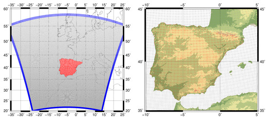
Figure 1.
Left: The domain of both experiments is marked with grey dots, and the relaxation zone for the model is highlighted in blue. Right: The mask defined for the IP is defined in red (also in left panel) over the topography of the region, as represented in the ETOPO1 dataset [64].
Besides the use of ERAI data as boundary and initial conditions for the model, a high resolution dataset NOAA OI SST v2 [65] was used to daily update the sea surface temperature (SST) of the model. The physical parameterizations included in both experiments are the following ones: five-class microphysics scheme (WSM5) [66], MYNN2 planetary boundary layer scheme [67], Tiedtke scheme for cumulus convection [68,69], RRTMG scheme for both long and shortwave radiation [70], and NOAH land surface model [71].
Before running the experiment including the 3DVAR data assimilation (WRF D), its background error covariance (BE) matrices were created using the CV5 method in WRFDA [72]. These matrices determine how the information provided by the assimilated observations should be spread to the nearby grid-points and vertical levels in the model, while the hydrostatic and geostrophic balances are imposed. A full description of the background error variances, their full vertical structure, and the algorithms used in the estimation of the optimum 3DVAR cost function can be found in Barker et al. [59,60]. The BE matrices vary monthly, and they are applicable only to this experiment as they take into account the chosen parameterizations and the domain. They were created from the data obtained from an independent 13-month simulation initialized at 12:00 a.m. and 12:00 p.m. UTC, and covering a different period to the one simulated (from January 2007 to February 2008). Each matrix is built using 90 days around the corresponding month, that is, the BE matrix for August is created using the data from July to September.
Both experiments presented here have already been validated against observational data in previous studies of the authors. The validation was carried out for variables such as precipitable water, precipitation, evaporation over the IP [73], and wind over the coastal areas [74], and this study presents the analysis of moisture recycling calculated using these thorough estimations of atmospheric moisture fields for the first time. In González-Rojí et al. [73], it was found that the experiment including data assimilation produced more reliable results than those obtained with the numerical integration where only boundary conditions drive the model (WRF N) for variables related to the water balance (e.g., precipitation, evaporation and precipitable water) over the IP. These results were sometimes superior, but always comparable, to those from ERAI. The water balance was also closed more efficiently by both WRF simulations than by ERAI, but particularly by the experiment with data assimilation. Additionally, WRF precipitation generated with 3DVAR data assimilation showed a similar performance as the one obtained by means of statistical downscaling [75]. Furthermore, as wind in this simulation showed also an improvement over ERAI, WRF outputs were used to calculate the offshore wind energy potential around the Mediterranean [74] and at every coast of the IP [76]. Due to the good results obtained by the experiment including 3DVAR data assimilation, the simulated period has been extended until the end of 2018 for the analysis of recycling ratio with a longer perspective.
2.2. Methodology
2.2.1. Definition of Moisture Recycling
The methodology that we follow is based on the moisture recycling defined by Eltahir and Bras in 1994. In Equation (6) from their paper [17], they define the spatial average of the recycling ratio for the total area of a basin and for any month k as:
where is the normalized precipitation at a given grid point and month k. Normalization is obtained by dividing by the total precipitation for that month in the basin. We can define the mean recycling ratio from a continuous field over a chosen area A following the previous approach using:
If we integrate the precipitation for the whole area, we know that
and we can rewrite Equation (2) as follows:
However, if we consider a Reynolds decomposition of the product in Equation (4), this equation is not totally true. Applying it to both precipitation and moisture recycling, we separate each value in mean and deviation from the spatial mean as commonly done:
with representing the areal mean of field X, and representing the deviations from the mean with . Thus, the mean of the product of both variables is:
This means that the covariance of spatial anomalies must be included in Equation (4), and the correct definition of the spatial average of moisture recycling should be:
2.2.2. Analysis
Once the definition of the moisture recycling is stated, we can start the analysis of the data. From previous studies of the authors [73], we know that WRF is not able to simulate correctly the evaporation over grid points defined as urban or built-up in the Noah land surface model. This is why we need to check whether considering these points in the analysis can trigger a bias in our results or not. To do so, we compare the areal mean of the monthly values of moisture recycling for both simulations (including or not the urban points) and we calculate the linear model between both values. If the results do no significantly differ, we will consider all the grid points included in the mask over the IP in order to provide a more complete study.
After that, we calculate the annual mean distribution of the monthly mean moisture recycling over the IP, and the spatial distribution of the values over the seasons. This will help us to characterize the moisture recycling over the IP in both simulations. Additionally, in order to distinguish the effect of 3DVAR data assimilation in the results, we also plot the monthly values obtained over the IP by means of a box-and-whisker diagram. This will help us to see the different distribution of the quantiles in both simulations.
In order to analyze the lead–lag structure of area-accumulated precipitation, areal mean soil moisture and mean moisture recycling, a Cross-Correlation Function (CCF) based analysis [77] was performed. In it, positive lags in soil moisture and moisture recycling are used to denote the response of these fields to previous values of precipitation.
3. Results
The comparison of the monthly mean moisture recycling values obtained with both simulations over the IP, including or not the urban points, is presented in Figure 2. It can be seen that differences associated with including or not all the values are really small. If we include in the analysis all grid points defined as urban in the land surface model, the monthly values are slightly higher than those without. However, the linear model between both options suggests that there is not a big difference between them. In both simulations, the slope of the linear regression is 1.04 and the intercept is 0.04. Additionally, the R-squared is also 1 (to 4 decimals), suggesting that both results are suitable for this study. For the completeness of the study, and in order to present results without excluding the values obtained around the urban areas, we decided to use all the grid points over the IP in the next steps of this paper. The reason for this is that the local underestimation of evaporation at a limited amount of grid points (urban category) does not severely affect the estimation of recycling over surrounding areas where other fields (precipitation and moisture transports) smooth the influence of these local evaporation errors.
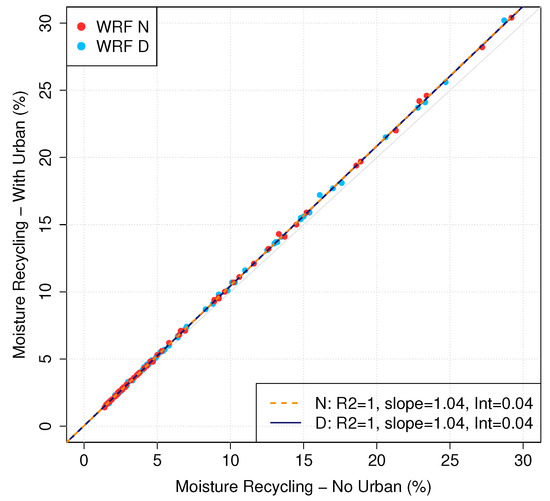
Figure 2.
Scatterplot of the monthly moisture recycling values computed including the urban points and without them. Points in red are obtained for the WRF N experiment (no data assimilation), while the blue ones are for WRF D. The linear models of both experiments are plotted in orange and dark blue, and the details of the slope and the intercept of each of them are included in the right bottom corner of the plot.
The mean annual cycle of moisture recycling and its interannual variability for period 2010–2014 is presented in Figure 3. Two different regimes are highlighted. During the extended winter, comprising November to February, the moisture recycling values are below 5%, suggesting that the interactions between atmosphere and land are limited. This is expected as winter months are the period of the year when many frontal systems affect the IP and the circulation is mainly zonal over the region [1,2,7] and the convective regimes that can trigger the moisture recycling are not favored. Additional studies about the sources of moisture affecting the IP [2] also point to the fact that, during this season, moisture sources are mainly located outside the IP. On the contrary, spring and summer are the seasons when the moisture recycling is important in the region, and the values are above 10%, a result also in agreement with previous results [2]. It is also important to point out the large variability of the results, particularly for spring, with standard deviations over 50%.
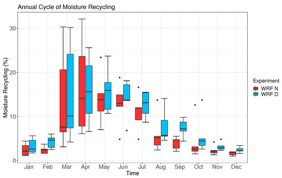
Figure 3.
Annual cycle of moisture recycling over the IP for both WRF simulations: WRF N in red and WRF D in blue.
If we compare both simulations, clear differences appear during summer and autumn. The moisture recycling values are smaller for the simulation without data assimilation, suggesting that the soil is really dry and that the 3DVAR data assimilation is able to correct this bias. The results corresponding to the soil moisture in the upper layer of the soil (see Figure S1 in Supplementary Materials) support this conclusion. If the mean values of each month are plotted instead of the variability of the monthly values as in Figure 3, the peak of the moisture recycling is observed in April for both simulations (16% and 17% for WRF N and WRF D, respectively). However, in the experiment without data assimilation, a secondary maximum is observed in October (mean value of 4.96%, while for September is 3.28% and 2.86% for November). According to previous studies [39], this maximum can be related to an increase in the number of convective events in the Mediterranean facade during late summer.
The results obtained are in agreement with previous studies. As stated before, the summer recycling ratio obtained by Bisselink and Dolman (2008) [44] ranged from 10 to 20%, and the mean value for July is around 6% according to Schär et al. (1999) [43]. Compared to Rios-Entenza et al., [38], the mean values for January and May are smaller in both simulations over the IP. However, if we compare our annual cycles to the one obtained by Rios-Entenza et al. (2014b) [39], a similar distribution is obtained, with high impact of the moisture recycling during spring and summer. Similar values are obtained in spring, but in winter the effect of the moisture recycling is even less important in our simulations. The greatest differences appear in autumn, but we cannot distinguish if they are due to different options (e.g., nesting with spectral nudging in the parent domain) and parameterizations used in the design of the experiments, or due to changes in the synoptic configuration before and after 2010 that can trigger the moisture recycling. Additionally, as those studies did not use any data assimilation scheme in their experiments, it is clear that their results are more similar to those obtained by experiment WRF N (without data assimilation) than to those obtained by WRF D.
The spatial distribution of moisture recycling for both simulations in winter (DJF), spring (MAM), summer (JJA), and autumn (SON) is presented in Figure 4. Additionally, the monthly accumulated precipitation maps are presented in Figure 5. Soil moisture maps can be found in the Supplementary Materials (see Figure S1), and they present a similar spatiotemporal variability to precipitation. The mean moisture transports over the IP (see Figure S2 in Supplementary Materials) show zonal flows, and the main difference between experiments is that the simulation with data assimilation produces slightly less intense flows than the one without.
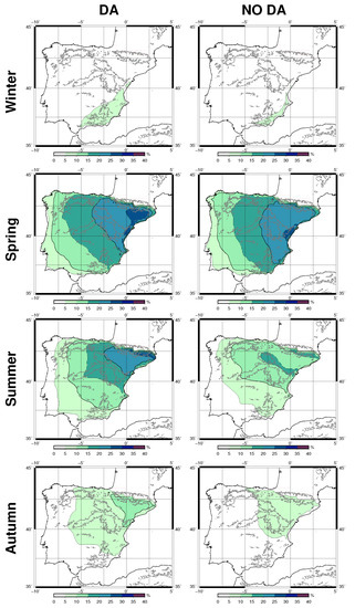
Figure 4.
Spatial distribution of moisture recycling in both WRF simulations (WRF D in the first column, and WRF N in the second one) along the different seasons: Winter (first row), Spring (second), Summer (third) and Autumn (fourth). The topography of the IP, as represented in the ETOPO1 dataset [64], is also included.
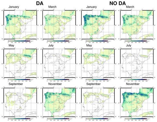
Figure 5.
Spatial distribution of accumulated precipitation (kg/m2 or mm) for different months of both WRF simulations; First, two columns belong to WRF D, and the other two to WRF N. The topography of the IP, as represented in the ETOPO1 dataset [64], is also included.
As expected from previous results, winter presents the smallest recycling values, with the simulation including data assimilation showing more efficiency towards inland of the IP than the one without data assimilation. For that season, the moisture recycling acts only in the southeastern corner of the IP, and small recycling ratios are observed in most regions of the IP (below 5%). At the same time, the precipitation amounts observed in those regions with low recycling ratios are more remarkable than in other months, particularly in the northwestern part of the IP. The differences between simulations are related to the fact that the experiment without data assimilation simulates more convective activity and/or orographic precipitation near the southeastern mountains of the IP than the experiment with it (see January), not favoring the conditions that can trigger the moisture recycling in that area. This result highlights the weak coupling between the surface and the atmosphere during winter, when the IP is dominated by zonal flows associated with large-scale systems (see Figure S2 in Supplementary Materials).
The highest values in both simulations are observed in spring, particularly for the simulation including data assimilation where the most intense recycling is located in the northeastern corner of the IP. In the case of the one without data assimilation, the maximum is located further south. The absence of the maximum of moisture recycling in WRF N in the northeastern corner of the IP is due to the different precipitation patterns in that region in both simulations. The experiment without data assimilation (WRF N) presents higher amounts of precipitation in that region (particularly in March), highlighting the influence of convective events and/or large scale features in the region. This is not observed in the simulation with data assimilation [73]. Additionally, the moisture recycling is also affected by the differences in soil moisture between simulations (see Figure S1). After a wet season, the soil is moist, but it gets drier as spring progresses, particularly for the simulation without data assimilation in the southern IP and near the Ebro basin. In May, the soil is dry in those regions in WRF N (values between 0.1 and 0.2 m3/m3), while in WRF D the soil is wetter (0.2 and 0.3 m3/m3).
The greatest differences between simulations are observed in summer. The simulation including data assimilation presents a pattern similar to the one in spring but with the maximum over the Pyrenees. On the contrary, the values of moisture recycling are smaller in the simulation without data assimilation, and the pattern highlights the importance of moisture recycling over the southern rims of the Ebro basin and in the Pyrenees. The precipitation is scarce in this season, and the differences are due to the soil moisture in both simulations (see Figure S1). Again, the experiment without data assimilation presents drier values than the one with data assimilation (between 0 and 0.1 m3/m3 for WRF N, and 0.1 and 0.2 m3/m3 for WRF D in most areas of the IP). The dryness of the soil is remarkable in the southwestern IP for WRF N, while the soil is particularly moist in WRF D near the Pyrenees and at the eastern section of the Cantabrian Range (see Figure S1). These regions are particularly those where the differences are observed in the moisture recycling.
Finally, autumn is a transition season between summer and winter and the values are again small. However, the values are even smaller for the simulation without data assimilation. The differences in precipitation patterns between both experiments are concentrated in late summer (September), and higher amounts of precipitation are observed near the mountainous regions in November. These differences in precipitation amounts and patterns are combined with the dryness of the soil in WRF N (see Figure S1), and this is why the moisture recycling is not so effective towards the southwestern corner of the IP in that simulation.
Compared to Rios-Entenza et al. (2014b) [39], similar patterns are observed, but with higher values in our simulations. Even if they show the spatial distribution of the moisture recycling monthly, a similar pattern to that observed in winter, spring and autumn can be detected in their results (Figure 7 from their manuscript), but particularly to WRF N. In autumn, when the differences between our both simulations are more evident, the patterns observed by them are also more similar to that obtained for the simulation without data assimilation. However, it must be pointed out again that their experiment did not include data assimilation, and this is why the pattern of their simulation and our WRF N experiment are more similar. If we compare the patterns obtained for spring in our study with the pattern for May from Rios-Entenza et al. [38] (Figure 7 in their paper), they are similar. However, due to the definition of their mask over the IP, we cannot distinguish where the maximum is going to appear in their case, and, therefore, to which of our simulations is more similar. However, their pattern resembles that obtained from WRF N, related also to the lack of using data assimilation in their experiment.
The variability of the areal mean seasonal values is presented in Figure 6 by means of a box and whiskers plot. Higher values of moisture recycling are obtained for the simulation including the data assimilation. However, the spread of the values is different depending on the season. In spring and summer, the spread of the values is bigger for WRF N, while, in autumn and winter, the spread is bigger for the simulation including data assimilation—WRF D. These results highlight the heterogeneity of the moisture recycling over the IP, both spatially and temporally.
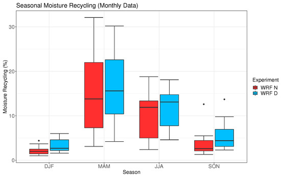
Figure 6.
Monthly values of moisture recycling for WRF N and WRF D (in red and blue, respectively) along each season.
Finally, due to the good capacity of the simulation including data assimilation to correct to some extent the bias in soil moisture observed between both simulations (presented in this study), and due to its ability to reproduce the spatial and temporal evolution of variables involved in the water balance as presented in previous studies by the authors [73,74,76], this simulation was extended until 2018. This is why this simulation (WRF D) was chosen to show the interannual variability of areal mean moisture recycling over the IP for the period 2010–2018. The temporal evolution can be found in Figure 7, along with those for areal mean soil moisture and accumulated precipitation.
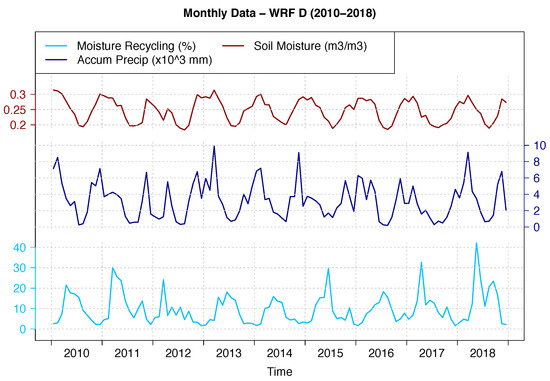
Figure 7.
Monthly values of moisture recycling, mean soil moisture, and accumulated precipitation over the IP for the period 2010–2018 only for the simulation including data assimilation.
The heterogeneity of the mean moisture recycling over the IP is highlighted in the results. It is clear that spring and summer are the most important seasons for the recycling, but particularly spring. The time series shows that the recycling has reached values near or above 30% during spring in some years (e.g., 2011, 2017, and 2018). However, it can be seen that this maximum can also be absent and the values can be below 20% during the entire year as in 2013, 2014 or 2016. Additionally, more than one secondary maximum in late summer can occur (e.g., 2012).
If we compare to Rios-Entenza et al. [39] (Figure 5 from their paper), we can see that the variability of the mean moisture recycling over the IP was also high from 1990–2007. Years without a maximum can be observed in 1991 or 2005, or years with more than one intense maximum as in 1997.
As shown in Figure 7, there exists a clear lead–lag relationship between precipitation and soil moisture and recycling. Thus, in order to determine the lag between each component involved in the moisture recycling, a Cross-Correlation Function (CCF) based analysis has been performed for each combination of the variables up to ten months. This analysis has covered the extended period simulated with WRF D (2010–2018—Figure 8), and also for both WRF simulations (Figure S3 in Supplementary Material) during a common period (2010–2014). Thus, we compare the behavior of lead–lag relationships with and without data assimilation.
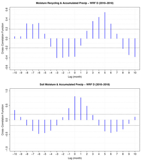
Figure 8.
Cross-Correlation Function (CCF) of moisture recycling against precipitation (top) and CCF of soil moisture against precipitation (bottom).
The top panel of Figure 8 shows the relationship between the moisture recycling and accumulated precipitation over the IP (WRF D experiment, 2010–2018). The maximum lagged CCF is observed when the lag is +5, suggesting that the moisture recycling achieves high values five months later than the maximum of precipitation accumulated over the IP, as also shown by Figure 7. In the case of soil moisture and accumulated precipitation (bottom panel), the lag corresponding to the highest value of the CCF is zero. Both figures support the interpretation that the mechanism linking the accumulation of moisture in the upper soil layer is very fast, while the conversion of that moisture into recycled precipitation happens at a much longer time-scale.
Figure S3 (in Supplementary Materials) shows the different behavior of the CCF functions (and therefore, the different dynamics of precipitation, soil moisture and moisture recycling) for WRF N and WRF D simulations. Figure S3 (top) shows that the moisture recycling for the WRF N experiment peaks at a four-months lag, while the peak happens at five months for the WRF D experiment. The plot in the middle shows that moisture recycling peaks at four months for the WRF D experiment, while it peaks at three months for WRF N. Finally, the CCF function for soil moisture (lagging) against precipitation peaks at a positive (+1 month) lag for the WRF N simulation, whilst it peaks at a zero lag for WRF D. As a general result from this figure, it can be seen that the CCF values for shorter lags are higher for the WRF N experiment. Conversely, for the WRF D experiment, the values at longer lags are higher. The interpretation corresponding to these results is that the soil moisture simulated by the NOAH model tends to underestimate the lifespan of soil moisture over the IP. This is somewhat corrected by the 3DVAR assimilation of atmospheric observations (soil moisture is not assimilated in our model configuration). These results support the idea that the simulation with data assimilation (WRF D) provides a better estimation of moisture recycling over the area.
4. Conclusions
This work analyses the effect of data assimilation on the moisture recycling over the IP for the period 2010–2014 comparing two simulations created with WRF. The first simulation is driven by boundary and initial conditions from ERAI. The second simulation is similar to the first experiment, but it also includes the 3DVAR data assimilation scheme four times a day. The outputs of both simulations were stored every 3 h, and the spatial resolution is 15 km.
The moisture recycling is a measurement of the relationships between the surface and atmosphere, and it depends on the evapotranspiration and precipitation measured over a region. For the calculation of the moisture recycling at each grid point of the domain, we extend the definition by Eltahir and Bras in 1994 [17] by explicitly considering the influence of covariances in the calculation of area-averaged moisture recycling (see Equation (7)).
The comparison of areal mean monthly values of moisture recycling over the IP including and omitting all the urban points from land surface model suggested that the differences are small in both simulations. This is why every grid point in the mask over the IP was included in this study.
The mean annual cycle of moisture recycling highlights two different regimes over the IP. The lowest values are obtained from November to February (around 3%), while the most remarkable values are observed in spring (around 16%) in both simulations. The lowest recycling ratios are associated with the highest precipitation amounts registered over the IP, particularly due to frontal systems coming from the Atlantic Ocean. The differences between both simulations are highlighted during summer and autumn. In those seasons, the soil is really dry in the simulation without data assimilation, but the 3DVAR data assimilation is able to correct this bias and produce smoother values.
If we focus on the seasonal patterns of moisture recycling, the heterogeneity of the IP is highlighted. In winter, the moisture recycling is confined to the southeastern corner of the IP with values up to 10%. In spring, the values are higher towards the Mediterranean coast, reaching values up to 25 or 30%. For the simulation including data assimilation, the maximum is in the northeastern corner of the IP, while the maximum is located further south for the simulation without data assimilation. The differences between simulations are remarkable in summer due to the differences in the soil moisture of the land surface model. In the case of the simulation without data assimilation, the soil is dryer and the moisture recycling is not so intense as in the simulation including data assimilation. Autumn is a transition season between summer and winter, and the moisture recycling reaches values around 10% in the northeastern corner of the IP.
The variability of the results is more important in spring and summer, and it is even higher for the simulation without data assimilation. This means that the annual cycle of moisture recycling can be different from one year to another, as it depends on the precipitation over the region and the synoptic scale circulation. This is observed in the time series of the areal mean of moisture recycling over the IP for the period 2010–2018. Some years with really intense maximums in spring are observed (e.g., 2011, 2017, or 2018), but also others with the total absence of this maximum (e.g., 2013 or 2014).
The analysis based on CCFs indicates that the data assimilation phase of the WRF D experiment extends the lifespan of moisture over the IP, thus introducing changes in the estimation of the moisture recycling if compared to the results obtained from the WRF N experiment. The underestimation of the lifespan of soil moisture over the IP in WRF N, together with the better verification statistics of precipitation, evaporation, and precipitable water [73], yields confidence in the fact that the estimation of moisture recycling from the WRF D experiment is better than the one from WRF N. For the extended WRF D simulation, it was found that the delay between precipitation and moisture recycling over the IP is five months.
Supplementary Materials
Figures S1–S3 are available online at the article’s website as a https://www.mdpi.com/2073-4433/11/1/19/s1. The data produced by the model needed to reproduce these results are publicly available, and they can be downloaded from https://doi.org/10.5281/zenodo.3529489.
Author Contributions
Conceptualization, S.J.G.-R., J.S., and G.I.-B.; methodology, S.J.G.-R. and J.S.; software, S.J.G.-R., J.S., and J.D.d.A.; investigation, S.J.G.-R. and J.S.; Preparation of datasets and analysis, all authors; writing—original-draft preparation, S.J.G.-R.; writing—review and editing, all authors; supervision, all authors; funding acquisition, S.J.G.-R., J.S., and G.I.-B. These authors contributed equally to this work. All authors have read and agreed to the published version of the manuscript.
Funding
S.J.G.-R. was supported by an FPI Predoctoral Research grant (MINECO, BES-2014-069977) during his PhD, and now he is funded by the Oeschger Centre for Climate Change Research. This work was also financially supported by the Spanish Government through MINECO project CGL2016-76561-R, (MINECO/ERDF, UE) and the University of the Basque Country (UPV/EHU, GIU 17/002).
Acknowledgments
S.J.G.-R. was supported by an FPI Predoctoral Research grant (MINECO, BES-2014-069977) during his PhD, and now he is funded by the Oeschger Centre for Climate Change Research. This work was also financially supported by the Spanish Government through MINECO project CGL2016-76561-R, (MINECO/ERDF, UE) and the University of the Basque Country (UPV/EHU, GIU 17/002). Intensive computational resources used in the project were provided by I2BASQUE. The authors thank the creators of the WRF/ARW and WRFDA systems for making them freely available to the community. Some of the calculations were carried out in the framework of R Core Team (2016). R: A language and environment for statistical computing. R Foundation for Statistical Computing, Vienna, Austria. https://www.R-project.org/.
Conflicts of Interest
The authors declare no conflict of interest.
Abbreviations
The following abbreviations are used in this manuscript:
| IP | Iberian Peninsula |
| ECMWF | European Centre for Medium-Range Weather Forecasts |
| WRF | Weather Research and Forecasting Model |
| NCEP | Centers for Environmental Prediction |
| GFS | Global Forecast System |
| GFDL | Geophysical Fluid Dynamics Laboratory |
| ERAI | ERA-Interim reanalysis |
| MARS | Meteorological Archival and Retrieval System |
| SST | Sea Surface Temperature |
| BE | Background Error covariance matrix |
| DJF | Winter |
| MAM | Spring |
| JJA | Summer |
| SON | Autumn |
| CCF | Cross-Correlation Function based analysis |
References
- Fernández, J.; Sáenz, J.; Zorita, E. Analysis of wintertime atmospheric moisture transport and its variability over southern Europe in the NCEP Reanalyses. Clim. Res. 2003, 23, 195–215. [Google Scholar] [CrossRef]
- Gimeno, L.; Nieto, R.; Trigo, R.M.; Vicente-Serrano, S.M.; López-Moreno, J.I. Where Does the Iberian Peninsula Moisture Come From? An Answer Based on a Lagrangian Approach. J. Hydrometeorol. 2010, 11, 421–436. [Google Scholar] [CrossRef]
- Gómez-Hernández, M.; Drumond, A.; Gimeno, L.; Garcia-Herrera, R. Variability of moisture sources in the Mediterranean region during the period 1980–2000. Water Resour. Res. 2013, 49, 6781–6794. [Google Scholar] [CrossRef]
- Sousa, P.M.; Trigo, R.M.; Barriopedro, D.; Soares, P.M.M.; Ramos, A.M.; Liberato, M.L.R. Responses of European precipitation distributions and regimes to different blocking locations. Clim. Dyn. 2017, 48, 1141–1160. [Google Scholar] [CrossRef]
- Rodríguez-Puebla, C.; Encinas, A.H.; Sáenz, J. Winter precipitation over the Iberian Peninsula and its relationship to circulation indices. Hydrol. Earth Syst. Sci. 2001, 5, 233–244. [Google Scholar] [CrossRef]
- Haylock, M.R.; Goodess, C.M. Interannual variability of European extreme winter rainfall and links with mean large-scale circulation. Int. J. Climatol. 2004, 24, 759–776. [Google Scholar] [CrossRef]
- Zveryaev, I.I.; Wibig, J.; Allan, R.P. Contrasting interannual variability of atmospheric moisture over Europe during cold and warm seasons. Tellus A 2008, 60, 32–41. [Google Scholar] [CrossRef]
- Rodriguez-Puebla, C.; Encinas, A.H.; Nieto, S.; Garmendia, J. Spatial and temporal patterns of annual precipitation variability over the Iberian Peninsula. Int. J. Climatol. 1998, 18, 299–316. [Google Scholar] [CrossRef]
- Sáenz, J.; Rodríguez-Puebla, C.; Fernández, J.; Zubillaga, J. Interpretation of interannual winter temperature variations over Southwestern Europe. J. Geophys. Res. Atmos. 2001, 106, 20641–20651. [Google Scholar] [CrossRef]
- Sáenz, J.; Zubillaga, J.; Rodríguez-Puebla, C. Interannual variability of winter precipitation in northern Iberian Peninsula. Int. J. Climatol. 2001, 21, 1503–1513. [Google Scholar] [CrossRef]
- Esteban-Parra, M.J.; Rodrigo, F.S.; Castro-Diez, Y. Spatial and temporal patterns of precipitation in Spain for the period 1880–1992. Int. J. Climatol. 1998, 18, 1557–1574. [Google Scholar] [CrossRef]
- Romero, R.; Ramis, C.; Guijarro, J. Daily rainfall patterns in the Spanish Mediterranean area: An objective classification. Int. J. Climatol. 1999, 19, 95–112. [Google Scholar] [CrossRef]
- Tullot, I.F. Climatología de España y Portugal; Universidad de Salamanca: Salamanca, Spain, 2000; Volume 76. [Google Scholar]
- Trigo, I.F.; Davies, T.D.; Bigg, G.R. Objective Climatology of Cyclones in the Mediterranean Region. J. Clim. 1999, 12, 1685–1696. [Google Scholar] [CrossRef]
- Quadrelli, R.; Pavan, V.; Molteni, F. Wintertime variability of Mediterranean precipitation and its links with large-scale circulation anomalies. Clim. Dyn. 2001, 17, 457–466. [Google Scholar] [CrossRef]
- Paredes, D.; Trigo, R.M.; Garcia-Herrera, R.; Trigo, I.F. Understanding Precipitation Changes in Iberia in Early Spring: Weather Typing and Storm-Tracking Approaches. J. Hydrometeorol. 2006, 7, 101–113. [Google Scholar] [CrossRef]
- Eltahir, E.A.B.; Bras, R.L. Precipitation recycling in the Amazon basin. Q. J. R. Meteorol. Soc. 1994, 120, 861–880. [Google Scholar] [CrossRef]
- Brubaker, K.L.; Entekhabi, D.; Eagleson, P.S. Estimation of Continental Precipitation Recycling. J. Clim. 1993, 6, 1077–1089. [Google Scholar] [CrossRef]
- Burde, G.I.; Zangvil, A. The Estimation of Regional Precipitation Recycling. Part I: Review of Recycling Models. J. Clim. 2001, 14, 2497–2508. [Google Scholar] [CrossRef]
- D’Odorico, P.; Porporato, A. Preferential states in soil moisture and climate dynamics. Proc. Natl. Acad. Sci. USA 2004, 101, 8848–8851. [Google Scholar] [CrossRef]
- Eltahir, E.A.B.; Bras, R.L. Precipitation recycling. Rev. Geophys. 1996, 34, 367–378. [Google Scholar] [CrossRef]
- Budyko, M.I.; Miller, D.H.; Miller, D.H. Climate and Life; Academic Press: New York, NY, USA, 1974; Volume 508. [Google Scholar]
- Burde, G.I.; Zangvil, A. The Estimation of Regional Precipitation Recycling. Part II: A New Recycling Model. J. Clim. 2001, 14, 2509–2527. [Google Scholar] [CrossRef]
- Bosilovich, M.G. On the vertical distribution of local and remote sources of water for precipitation. Meteorol. Atmos. Phys. 2002, 80, 31–41. [Google Scholar] [CrossRef]
- Burde, G.I. Bulk Recycling Models with Incomplete Vertical Mixing. Part I: Conceptual Framework and Models. J. Clim. 2006, 19, 1461–1472. [Google Scholar] [CrossRef]
- Burde, G.I.; Gandush, C.; Bayarjargal, Y. Bulk Recycling Models with Incomplete Vertical Mixing. Part II: Precipitation Recycling in the Amazon Basin. J. Clim. 2006, 19, 1473–1489. [Google Scholar] [CrossRef]
- Dominguez, F.; Kumar, P.; Liang, X.Z.; Ting, M. Impact of Atmospheric Moisture Storage on Precipitation Recycling. J. Clim. 2006, 19, 1513–1530. [Google Scholar] [CrossRef]
- Dirmeyer, P.A.; Brubaker, K.L. Characterization of the Global Hydrologic Cycle from a Back-Trajectory Analysis of Atmospheric Water Vapor. J. Hydrometeorol. 2007, 8, 20–37. [Google Scholar] [CrossRef]
- Bosilovich, M.G.; Schubert, S.D. Precipitation Recycling over the Central United States Diagnosed from the GEOS-1 Data Assimilation System. J. Hydrometeorol. 2001, 2, 26–35. [Google Scholar] [CrossRef]
- Szeto, K.K. Moisture recycling over the Mackenzie basin. Atmosphere-Ocean 2002, 40, 181–197. [Google Scholar] [CrossRef]
- Serreze, M.C.; Bromwich, D.H.; Clark, M.P.; Etringer, A.J.; Zhang, T.; Lammers, R. Large-scale hydro- climatology of the terrestrial Arctic drainage system. J. Geophys. Res. Atmos. 2002, 107, 8160. [Google Scholar] [CrossRef]
- Trenberth, K.E. Atmospheric Moisture Recycling: Role of Advection and Local Evaporation. J. Clim. 1999, 12, 1368–1381. [Google Scholar] [CrossRef]
- Bosilovich, M.G.; Schubert, S.D. Water Vapor Tracers as Diagnostics of the Regional Hydrologic Cycle. J. Hydrometeorol. 2002, 3, 149–165. [Google Scholar] [CrossRef]
- Berbery, E.H.; Rasmusson, E.M. Mississippi Moisture Budgets on Regional Scales. Mon. Weather Rev. 1999, 127, 2654–2673. [Google Scholar] [CrossRef]
- Gutowski, W.J.; Chen, Y.; Ötles, Z. Atmospheric Water Vapor Transport in NCEP–NCAR Reanalyses: Comparison with River Discharge in the Central United States. Bull. Am. Meteorol. Soc. 1997, 78, 1957–1970. [Google Scholar] [CrossRef]
- Higgins, R.W.; Mo, K.C.; Schubert, S.D. The Moisture Budget of the Central United States in Spring as Evaluated in the NCEP/NCAR and the NASA/DAO Reanalyses. Mon. Weather Rev. 1996, 124, 939–963. [Google Scholar] [CrossRef]
- Trenberth, K.E.; Guillemot, C.J. Evaluation of the atmospheric moisture and hydrological cycle in the NCEP/NCAR reanalyses. Clim. Dyn. 1998, 14, 213–231. [Google Scholar] [CrossRef]
- Rios-Entenza, A.; Miguez-Macho, G. Moisture recycling and the maximum of precipitation in spring in the Iberian Peninsula. Clim. Dyn. 2014, 42, 3207–3231. [Google Scholar] [CrossRef]
- Rios-Entenza, A.; Soares, P.M.M.; Trigo, R.M.; Cardoso, R.M.; Miguez-Macho, G. Moisture recycling in the Iberian Peninsula from a regional climate simulation: Spatiotemporal analysis and impact on the precipitation regime. J. Geophys. Res. Atmos. 2014, 119, 5895–5912. [Google Scholar] [CrossRef]
- Skamarock, W.C.; Klemp, J.B.; Dudhia, J.; Gill, D.O.; Barker, D.M.; Duda, M.G.; Huang, X.Y.; Wang, W.; Powers, J.G. A Description of the Advanced Research WRF Version 3; NCAR Technical Note NCAR/TN-475+STR; University Corporation for Atmospheric Research: Boulder, CO, USA, 2008. [Google Scholar] [CrossRef]
- Dee, D.P.; Uppala, S.M.; Simmons, A.J.; Berrisford, P.; Poli, P.; Kobayashi, S.; Andrae, U.; Balmaseda, M.A.; Balsamo, G.; Bauer, P.; et al. The ERA-Interim reanalysis: Configuration and performance of the data assimilation system. Q. J. R. Meteorol. Soc. 2011, 137, 553–597. [Google Scholar] [CrossRef]
- van der Ent, R.J.; Savenije, H.H.G.; Schaefli, B.; Steele-Dunne, S.C. Origin and fate of atmospheric moisture over continents. Water Resour. Res. 2010, 46. [Google Scholar] [CrossRef]
- Schär, C.; Lüthi, D.; Beyerle, U.; Heise, E. The Soil–Precipitation Feedback: A Process Study with a Regional Climate Model. J. Clim. 1999, 12, 722–741. [Google Scholar] [CrossRef]
- Bisselink, B.; Dolman, A.J. Precipitation Recycling: Moisture Sources over Europe using ERA-40 Data. J. Hydrometeorol. 2008, 9, 1073–1083. [Google Scholar] [CrossRef]
- Dirmeyer, P.A.; Brubaker, K.L.; DelSole, T. Import and export of atmospheric water vapor between nations. J. Hydrol. 2009, 365, 11–22. [Google Scholar] [CrossRef]
- Fitzmaurice, J.A. A Critical Analysis of Bulk Precipitation Recycling Models. Ph.D. Thesis, Massachusetts Institute of Technology, Cambridge, MA, USA, 2007. [Google Scholar]
- Keys, P.W.; van der Ent, R.J.; Gordon, L.J.; Hoff, H.; Nikoli, R.; Savenije, H.H.G. Analyzing precipitationsheds to understand the vulnerability of rainfall dependent regions. Biogeosciences 2012, 9, 733–746. [Google Scholar] [CrossRef]
- van der Ent, R.J.; Tuinenburg, O.A.; Knoche, H.R.; Kunstmann, H.; Savenije, H.H.G. Should we use a simple or complex model for moisture recycling and atmospheric moisture tracking? Hydrol. Earth Syst. Sci. 2013, 17, 4869–4884. [Google Scholar] [CrossRef]
- Goessling, H.F.; Reick, C.H. On the “well-mixed” assumption and numerical 2D tracing of atmospheric moisture. Atmos. Chem. Phys. 2013, 13, 5567–5585. [Google Scholar] [CrossRef]
- Yoshimura, K.; Oki, T.; Ichiyanagi, K. Evaluation of two-dimensional atmospheric water circulation fields in reanalyses by using precipitation isotopes databases. J. Geophys. Res. Atmos. 2004, 109. [Google Scholar] [CrossRef]
- Kurita, N.; Yoshida, N.; Inoue, G.; Chayanova, E.A. Modern isotope climatology of Russia: A first assessment. J. Geophys. Res. Atmos. 2004, 109. [Google Scholar] [CrossRef]
- Gat, J.R. Atmospheric water balance—The isotopic perspective. Hydrol. Process. 2000, 14, 1357–1369. [Google Scholar] [CrossRef]
- Aggarwal, P.K.; Alduchov, O.; Araguás Araguás, L.; Dogramaci, S.; Katzlberger, G.; Kriz, K.; Kulkarni, K.M.; Kurttas, T.; Newman, B.D.; Purcher, A. New capabilities for studies using isotopes in the water cycle. Eos Trans. Am. Geophys. Union 2007, 88, 537–538. [Google Scholar] [CrossRef]
- Nieto, R.; Gimeno, L.; Trigo, R.M. A Lagrangian identification of major sources of Sahel moisture moisture. Geophys. Res. Lett. 2006, 33. [Google Scholar] [CrossRef]
- Stohl, A.; James, P. A Lagrangian Analysis of the Atmospheric Branch of the Global Water Cycle. Part I: Method Description, Validation, and Demonstration for the August 2002 Flooding in Central Europe. J. Hydrometeorol. 2004, 5, 656–678. [Google Scholar] [CrossRef]
- Stohl, A.; James, P. A Lagrangian Analysis of the Atmospheric Branch of the Global Water Cycle. Part II: Moisture Transports between Earth’s Ocean Basins and River Catchments. J. Hydrometeorol. 2005, 6, 961–984. [Google Scholar] [CrossRef]
- Argüeso, D.; Hidalgo-Muñoz, J.M.; Gámiz-Fortis, S.R.; Esteban-Parra, M.J.; Dudhia, J.; Castro-Díez, Y. Evaluation of WRF Parameterizations for Climate Studies over Southern Spain Using a Multistep Regionalization. J. Clim. 2011, 24, 5633–5651. [Google Scholar] [CrossRef]
- Zheng, D.; Van Der Velde, R.; Su, Z.; Wen, J.; Wang, X. Assessment of Noah land surface model with various runoff parameterizations over a Tibetan river. J. Geophys. Res. Atmos. 2017, 122, 1488–1504. [Google Scholar] [CrossRef]
- Barker, D.M.; Huang, W.; Guo, Y.R.; Bourgeois, A.J.; Xiao, Q.N. A Three-Dimensional Variational Data Assimilation System for MM5: Implementation and Initial Results. Mon. Weather Rev. 2004, 132, 897–914. [Google Scholar] [CrossRef]
- Barker, D.; Huang, X.Y.; Liu, Z.; Auligné, T.; Zhang, X.; Rugg, S.; Ajjaji, R.; Bourgeois, A.; Bray, J.; Chen, Y.; et al. The Weather Research and Forecasting Model’s Community Variational/Ensemble Data Assimilation System: WRFDA. Bull. Am. Meteorol. Soc. 2012, 93, 831–843. [Google Scholar] [CrossRef]
- National Centers for Environmental Prediction/National Weather Service/NOAA/U.S. Department of Commerce. NCEP ADP Global Upper Air and Surface Weather Observations (PREPBUFR Format); National Center for Atmospheric Research, Computational and Information Systems Laboratory: Boulder, CO, USA, 2008. [Google Scholar] [CrossRef]
- Rummukainen, M. State-of-the-art with regional climate models. Wiley Interdiscip. Rev. Clim. Chang. 2010, 1, 82–96. [Google Scholar] [CrossRef]
- Jones, R.G.; Murphy, J.M.; Noguer, M. Simulation of climate change over europe using a nested regional-climate model. I: Assessment of control climate, including sensitivity to location of lateral boundaries. Q. J. R. Meteorol. Soc. 1995, 121, 1413–1449. [Google Scholar] [CrossRef]
- Amante, C.; Eakins, B. ETOPO1 1 Arc-Minute Global Relief Model: Procedures, Data Sources and Analysis; NOAA Technical Memorandum NESDIS NGDC-24; National Geophysical Data Center, NOAAL: Boulder, CO, USA, 2009.
- Reynolds, R.W.; Smith, T.M.; Liu, C.; Chelton, D.B.; Casey, K.S.; Schlax, M.G. Daily High-Resolution-Blended Analyses for Sea Surface Temperature. J. Clim. 2007, 20, 5473–5496. [Google Scholar] [CrossRef]
- Hong, S.Y.; Dudhia, J.; Chen, S.H. A Revised Approach to Ice Microphysical Processes for the Bulk Parameterization of Clouds and Precipitation. Mon. Weather Rev. 2004, 132, 103–120. [Google Scholar] [CrossRef]
- Nakanishi, M.; Niino, H. An Improved Mellor–Yamada Level-3 Model: Its Numerical Stability and Application to a Regional Prediction of Advection Fog. Bound.-Layer Meteorol. 2006, 119, 397–407. [Google Scholar] [CrossRef]
- Tiedtke, M. Comprehensive Mass Flux Scheme for Cumulus Parameterization in Large-Scale Models. Mon. Weather Rev. 1989, 117, 1779–1800. [Google Scholar] [CrossRef]
- Zhang, C.; Wang, Y.; Hamilton, K. Improved Representation of Boundary Layer Clouds over the Southeast Pacific in ARW-WRF Using a Modified Tiedtke Cumulus Parameterization Scheme. Mon. Weather Rev. 2011, 139, 3489–3513. [Google Scholar] [CrossRef]
- Iacono, M.J.; Delamere, J.S.; Mlawer, E.J.; Shephard, M.W.; Clough, S.A.; Collins, W.D. Radiative forcing by long-lived greenhouse gases: Calculations with the AER radiative transfer models. J. Geophys. Res. Atmos. 2008, 113. [Google Scholar] [CrossRef]
- Tewari, M.; Chen, F.; Wang, W.; Dudhia, J.; LeMone, M.; Mitchell, K.; Ek, M.; Gayno, G.; Wegiel, J.; Cuenca, R. Implementation and verification of the unified NOAH land surface model in the WRF model. In Proceedings of the 20th Conference on Weather Analysis and Forecasting/16th Conference on Numerical Weather Prediction, Seattle, WA, USA, 10–12 January 2004; Volume 1115. [Google Scholar]
- Parrish, D.F.; Derber, J.C. The National Meteorological Center’s Spectral Statistical-Interpolation Analysis System. Mon. Weather Rev. 1992, 120, 1747–1763. [Google Scholar] [CrossRef]
- González-Rojí, S.J.; Sáenz, J.; Ibarra-Berastegi, G.; Díaz de Argandoña, J. Moisture balance over the Iberian Peninsula according to a regional climate model: The impact of 3DVAR data assimilation. J. Geophys. Res. Atmos. 2018, 123, 708–729. [Google Scholar] [CrossRef]
- Ulazia, A.; Sáenz, J.; Ibarra-Berastegui, G.; González-Rojí, S.J.; Carreno-Madinabeitia, S. Using 3DVAR data assimilation to measure offshore wind energy potential at different turbine heights in the West Mediterranean. Appl. Energy 2017, 208, 1232–1245. [Google Scholar] [CrossRef]
- González-Rojí, S.J.; Wilby, R.L.; Sáenz, J.; Ibarra-Berastegi, G. Harmonized evaluation of daily precipitation downscaled using SDSM and WRF+WRFDA models over the Iberian Peninsula. Clim. Dyn. 2019, 53, 1413–1433. [Google Scholar] [CrossRef]
- Ulazia, A.; Ibarra-Berastegi, G.; Sáenz, J.; Carreno-Madinabeitia, S.; González-Rojí, S.J. Seasonal Correction of Offshore Wind Energy Potential due to Air Density: Case of the Iberian Peninsula. Sustainability 2019, 11, 3648. [Google Scholar] [CrossRef]
- Probst, W.N.; Stelzenmüller, V.; Fock, H.O. Using cross-correlations to assess the relationship between time-lagged pressure and state indicators: An exemplary analysis of North Sea fish population indicators. ICES J. Mar. Sci. 2012, 69, 670–681. [Google Scholar] [CrossRef]
© 2019 by the authors. Licensee MDPI, Basel, Switzerland. This article is an open access article distributed under the terms and conditions of the Creative Commons Attribution (CC BY) license (http://creativecommons.org/licenses/by/4.0/).