Abstract
The influence of urbanization on regional precipitation is one of the most important issues in hydrology. This paper selected the North Haihe Basin as the study area and explored the connection between summer precipitation and urbanization index (URBI) based on satellite precipitation and nighttime lights datasets. A moving spatial percentage anomaly method (MSP) was used to signify the local induced enhancement of precipitation (LIEP). Local indicators of spatial association (LISA) clustering for LIEP and URBI based on Bivariate Moran’s I coupled with digital elevation model (DEM) segmentation was used to separate the impacts caused by urbanization and terrain uplifting, and thus, the regions of interest (ROI) where the urban induced enhancement of precipitation (UIEP) plays a dominant role were located. A geographically weighted regression (GWR) model was used to reveal the spatial variation of the sensitivity of UIEP to URBI within the ROI. Pearson correlation and cross-wavelet analyses (XWT) were adopted to investigate the teleconnection between UIEP and climate anomalies, using Niño3.4 and SOI as indices. The results indicated that: (1) Urbanization effects on precipitation spatial variation in the upstream mountainous area would be hidden away by topographic factors. (2) From the perspective of the basin, the highest urbanization level areas have the Lowest LIEP, while the suburban areas have the highest LIEP, and the rural areas are in the middle. (3) The UIEP and the URBI are generally negatively correlated within ROI. (4) UIEP versus Niño3.4 and SOI both show a significant common high-power period at a time scale of 2 years. This work can help comprehensively understand the hydrological response to urbanization.
1. Introduction
Precipitation is one of the most basic hydro-meteorological elements. Researchers have been aware of the urban influence on precipitation for many years [1,2,3]. However, many different viewpoints on the possible mechanisms related to urbanization-induced precipitation alterations still exist [3]. In the past few decades, human society has experienced a rapid urbanization process, and this trend is predicted to continue [4,5]. Thus, the influence of urbanization on regional precipitation has aroused many people’s interests [6,7,8].
At present, studies of urban impacts on precipitation are commonly based on either observational data or numerical models. Observational data mainly involve rain-gauge data [9,10], remote sensing precipitation products [11], and radar quantitative precipitation estimation products [12]. Compared to the urban heat island (UHI) effect, urban effects on precipitation are not always concentrated in the city but change with various geographical conditions and climate backgrounds (a dry or wet climate situation). To evaluate urbanization impacts on zonal precipitation, a statistical analysis based on long-term observations of rainfall data is an acceptable way to distinguish likely influenced areas, which are not perfectly centered in the city [13]. For numerical simulations, mesoscale meteorological models such as the Weather Research and Forecasting Model (WRF) and the PSU/NCAR mesoscale model (MM5) have been widely applied [14,15,16]. The main approach of theses simulations is either to modify the surface process parameters in the urban region—such as albedo, roughness, and soil thermal properties—or to be coupled with single-layer urban canopy models (UCM) and multi-layer UCMs to offer explicit urban considerations. UCM can represent urban areas for a more accurate estimation of 2 m air temperature, 10 m wind speed, 2 m relative humidity, precipitation, surface temperature, and shortwave and longwave radiation, while multi-layer UCMs can represent cities with very high buildings and high variability. Most research results suggest that urbanization can influence regional precipitation by altering dynamic meteorological conditions [17], thereby enhancing the rainfall amount and frequency in the urban and the urban downwind area to some extent [10,18,19]. However, because the precipitation process tends to exhibit complexity, discontinuity, and strong regional features, considerably different results have been concluded in different studies. For example, Ref. [16] found that the precipitation amount in Guangzhou city showed a significant increasing trend that was not found in nearby suburban and rural areas. In contrast, Ref. [20] detected that the precipitation amount in most cities of the Beijing-Tianjin-Hebei region showed a downward trend, and the authors thought this was caused by an extreme-precipitation (≥50 mm/d) decrease [21].
Current studies about urban impacts on precipitation are concentrated on both single cities and city agglomerations [7,11,22,23]. The general research measure is to compare the rainfall attributes between urban areas and nearby suburban areas to validate urban effects on precipitation. However, the relationship between the central city and suburban areas in most research has been generalized as a type of point–point relation, and there is a lack of further analysis on the spatial response relationship between rainfall field and urbanization level distribution at both the basin and city cluster scale. One objective of this paper is to distinguish sections where precipitation variation is mainly influenced by urban development in the north Haihe basin and to explore the precipitation variation’s sensitivity to the urbanization index (URBI) in these areas. To achieve this goal, a moving spatial percentage anomaly (MSP) method was used to quantify the local induced enhancement of precipitation (LIEP) based on a satellite precipitation product. Bivariate Moran’s I for LIEP and the urban level index were adopted to extract the region of interest (ROI), where the LIEP is equivalent to the urban induced enhancement of precipitation (UIEP). Geographically weighted regression (GWR) was applied in ROI to explore the UIEP’s sensitivity to urban level.
In addition to the relationship between the rainfall field and urbanization spatial distribution, some studies [22,24,25] have shown that the degree of rainfall variation caused by urbanization was closely related to climate background (wetter or direr conditions). Ref. [25] simulated the summer rainfall in the Beijing-Tianjin-Hebei metropolis during extreme dry and wet years (1994 and 1997) using WRF coupled with UCM. By comparing the simulation results in these two situations, they found that the retardation of convective activity induced by the “dry island effect” turned out to be greater than the augmentation of the convergence from both the urban “heat island effect” and the urban canopy roughness in the wet year (1994), which induced a rainfall decrease in urban areas and most of their surrounding areas. Very few studies have analyzed the relationship between UIEP and climate background based on long time regional rainfall series statistical analyses. It has been believed that El Niño southern oscillation (ENSO) had great impacts on the climate in many areas of the world through global teleconnections [26]. The regional climate background change can thus be reflected by ENSO. Therefore, the second aim of this paper is to explore the connection between the strength of UIEP and the climate anomalies ENSO. To this end, Empirical orthogonal function (EOF), Pearson’s correlation, and wavelet analyses were utilized to reveal the linear and nonlinear relationship between the climate background and UIEP.
2. Materials and Methods
2.1. Study Area
This study takes the north part of the Haihe Basin as the study area (Figure 1). The study area is located between 112°~120° E longitude and 38°~43° N latitude, facing the Bohai sea in the east, and the Inner Mongolian Plateau in the north. To the west is the Taihang Mountain and to the south is the North China plain. The area’s climate covers semi-humid and semiarid continental monsoons. Under the influence of the East Asian summer monsoon (EASM) and the terrain conditions, the spatial and temporal distribution of precipitation shows clear zonal, seasonal, and inter-annual variation [27,28,29]. The average precipitation is 550 mm, most of which is concentrated in summer (June, July, and August, JJA). The study area is densely populated with large and medium-sized cities, among which Beijing, Tianjin and their surrounding cities are the core area of the Beijing-Tianjin-Hebei city cluster, one of the three major metropolitan areas of China.
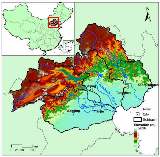
Figure 1.
Locations of the study area.
2.2. Data Acuisition
In this paper, The Tropical Rainfall Measuring Mission (TRMM) multi-Satellite precipitation analysis products 3B43 V7 [30] from 1998 to 2018 were used. The resolution is 0.25° × 0.25° [31]. It has been validated that the TRMM 3B43 data are of high adaptability in the Haihe basin [23]. The Digital Elevation Model (DEM) dataset was provided by the Geospatial Data Cloud site, Computer Network Information Center, Chinese Academy of Sciences [32], with a 90 m × 90 m resolution. The Defense Meteorological Satellite Program/Operational Linescan System [33] nighttime lights time series V4 acquired from NOAA’s National Geophysical Data Center was applied to represent the urbanization level in the study area, which has a resolution of 1 km × 1 km [34,35]. The DMSP/OLS nighttime lights data have been widely adopted to quantize the urbanization level in studies related to urban issues [35,36,37,38]. These data can detect low-intensity lights in urban areas and distinguish them from dark rural backgrounds, thus, they are suitable to be used as an urbanization index (URBI). Considering that urban sprawl is relatively insignificant against the entire basin’s background, and since the study period is not too long, the DMSP/OLS nighttime lights data of 2010 were used over the entire study period for simplicity. In this study, all the above data are resampled into 0.25° × 0.25°. The NCEP monthly mean wind reanalysis data provided by the NOAA Earth System Research Laboratory, Physical Sciences Division (NOAA/OAR/ESRL PSD), Boulder, Colorado, USA, from their Web site at https://www.esrl.noaa.gov/ [39], were used to obtain the summer mean wind direction, with a resolution of 2.5° × 2.5°.
2.3. Methodology
2.3.1. Empirical Orthogonal Function (EOF) Analysis
The empirical orthogonal function (EOF) and the principal components analysis (PCA) were sometimes used to describe the same method [40], but EOF can emphasize both temporal coefficient and spatial pattern [41]. The EOF was applied to realize the decomposition of the summer precipitation, and both spatial patterns and temporal coefficients were obtained. The spatial patterns represent the main spatial feature of summer precipitation, and the temporal coefficients are the principal components.
The EOF is based on the estimation of the eigenvalues and eigenvectors of an anomaly covariance matrix of the precipitation field. The derived eigenvalues provide a measure of the percent variance explained by each spatial pattern. North’s test [42] is selected to determine if a particular eigenvalue (pattern) is distinct from its nearest neighbor.
The purpose of the EOF analysis is to compare the obtained main spatial pattern of summer precipitation with urbanization spatial distribution delineated by nighttime lights data. The result can offer a preliminary assessment of urbanization influence on the spatial rainfall patterns at the basin scale. The EOF analysis was also used in the decomposition of the urban induced enhancement of the precipitation index (UIEP), and temporal coefficients of the first EOF pattern were used as a substitution for the UIEP field in the correlation analysis with climate anomalies.
2.3.2. Local Induced Enhancement of Precipitation
This article uses a moving spatial percentage anomaly (MSP) to signify the local high/low points; this is a filtering process [43,44]. Assuming that the climate change beyond the moving-window scale is caused by large-scale natural climate forces, then the uneven spatial distribution after filtering can be attributed to the effects of local climate forces (such as urbanization, land use change, abrupt terrain change, and anthropogenic aerosol emissions). The value of MSP was taken as the LIEP index. The steps for calculating LIEP using MSP are as follows. First, a rectangular moving window with certain size (larger than 0.25° × 0.25°) centered on each cell of the TRMM 3B43 data was introduced. Second, for every year, the mean summer rainfall Pmean within the whole window and the mean rainfall Pc on the central cell were calculated. Then, the percentage difference between the central cell value Pc and the Pmean can be easily obtained as the LIEP:
If the LIEP value is positive, then the local elements enhance the precipitation, where the corresponding region tends to have a “wet island effect”. On the contrary, if the LIEP value is negative, then the local elements inhibited the precipitation, where the corresponding region tends to show a “dry island effect”. If the LIEP value is zero, the local elements’ effects are not obvious.
In the method mentioned above, the moving window’s size would definitely impact the results of the rainfall’s spatial heterogeneity. In order to reasonably determine the scope of the moving window, a spatial auto-correlation analysis of the precipitation in different years was carried out. The spatial autocorrelation of the precipitation would remain positive and strong within a certain distance, which suggested that the precipitation within a limited range tended to be affected by the same local climate force. The spacing within which the autocorrelation of precipitation remains positive was thus determined to be in the range of the moving window.
2.3.3. Bivariate Moran’s I
Besides the urbanization factor, there exist transitions from plains to mountains in the study area, where the topography uplift may have a greater impact on local precipitation. The bivariate Moran’s I [45,46] for the LIEP versus Urbanization index was adopted to extract the region where the urban effect may play a dominant role in influencing precipitation.
The bivariate Moran’s I is extended from the traditional method of Moran’s I and can identify the clustering of extreme values between two variants. The bivariate Moran’s I is defined as in Equation (2):
where indicates the value of feature k on space unit i; indicates the value of feature l on space unit j; and are the mean value of feature k and l, respectively; is the spatial weight between these two features; and S2 is the covariance of features k and l.
The bivariate Local Moran’s I has been used to produce local indicators of spatial association (LISA) measure. The calculation of bivariate Local Moran’s I is shown in Equation (3):
where and are the observed variance of feature k and l, respectively. It is worth noting that the bivariate Moran’s I does not suggest an in-place inherent correlation between and , but instead between and .
Through the LISA cluster map, prepared with Geoda [47,48] (http://geodacenter.github.io), locations with significant local Moran’s statistics can be obtained. We are interested in the cluster types with a High LIEP value versus a high urban level (H-H) and a Low LIEP value versus a high urban level (L-H). Coupled with the DEM data, areas with large topographic uplift need to be removed to exclude the interference of topography alteration elements. Then, the region of interest (ROI) can be obtained, where the LIEPs are considered to be dominantly caused by the urbanization factor (land use change, anthropogenic aerosol emissions, etc.) and are thus expressed as the Urban induced enhancement of precipitation (UIEP).
2.3.4. Geographically Weighted Regression, GWR
The geographic weighted regression model (GWR) is an extension of ordinary least squares regression (OLS) and adds a level of modeling sophistication by allowing the relation between the independent and dependent variables to vary by locality. GWR constructs a separate OLS equation for every location in the dataset, which incorporates the dependent and explanatory variables of the locations falling within the bandwidth of each target location [49,50,51]. The bandwidth is the key controlling parameter in the weighting scheme, which can be optimized by the Akaike Information Criterion (AIC) [52]. This paper uses the GWR model to interpret the spatial variation of the sensitivity of UIEP to URBI.
2.3.5. Pearson Correlation and Cross-Wavelet Analysis
The Pearson correlation is used to investigate a simple linear relation. In order to further reveal the specific details of the non-linear relation from both the time domain and frequency domain, a cross-wavelet analysis (XWT) was adopted. XWT is an effective tool for exploring the correlations between two time series, as it combines the characteristics of wavelet transform and cross spectrum analysis. If the wavelet transforms of the xt and yt series are and , respectively, the cross-wavelet spectrum can be expressed as Equation (4) [53]:
where s and t, respectively, denote the scale expansion factor and the time shift factor, and the * refers to complex conjugation. The modulus of the cross-wavelet transform indicates the cross-amplitude, where a larger value indicates a higher degree of correlation.
The phase difference between these two series for a given delay time and a specific scale can be defined as Equation (5):
where S is the smooth operator and R and I represent the real and imaginary parts of the cross-wavelet spectrum.
3. Results and Discussion
3.1. The Summer Rainfall Spatial Distribution Characteristics in North Haihe Basin
For the purpose of understanding the spatial and temporal distribution characteristics of the summer rainfall, an EOF analysis was performed on the 3B43 precipitation data. The first three spatial patterns and their corresponding temporal coefficients are shown in Figure 2. Their cumulative variance contribution rate is 0.7 and passes North’s test [42], which indicates that these eigenvalues are significantly separated.
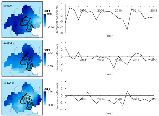
Figure 2.
The first three spatial pattern and their corresponding temporal coefficients of the summer rainfall in study area by an empirical orthogonal function (EOF) analysis. (a–c) represent respectively the first leading spatial pattern, the second leading spatial pattern and the third leading spatial pattern.
As shown in Figure 2, the spatial pattern of the first leading spatial pattern (EOF1) mainly reflects the gradual precipitation amount changes from the coastal to inland and also from plain to mountainous areas. These gradual changes eventually lead to the distinct difference in precipitation distribution between the mountainous upstream area and the flat middle and downstream area. The correlation coefficient between the temporal coefficient of the first pattern (PC1) and the average summer precipitation amount of the basin reaches −0.57 (at a significance level of 0.01). This may be related to the control of large-scale weather systems in the summer. Since the PC1 is entirely negative, the negative loading region in EOF1 from middle and downstream areas to Bohai gulf contributes to large portions of the basin’s precipitation.
The second EOF pattern (EOF2) shows an obvious south-to-north reverse change. Combined with the temporal coefficient (PC2), this pattern reveals the fact that there are more chances for the south region to have greater precipitation. Both the distributions of EOF1 and EOF2 are related to the large-scale climate background and geographical environment.
However, in the third EOF pattern (EOF3), heavier negative loading is located at the north of Tianjin and the northeast of Beijing. This location is coincident with the windward slope of the mountains in the north Haihe basin, and this area is also the downwind area of Beijing-Tianjin (shown in Figure 3; the downwind area is located in the northeast of these two cities). This might be the consequence of the bifactor functioning of topographic forces and urban effects. Within the plain area at the southeast of the study area, the loading in both the Beijing–Tianjin urban and peri-urban areas shows a slight spatial difference with the exterior zone. Compared to prior patterns, the EOF3 reflects the spatial difference of precipitation induced by local climate forces. Taken together, the contribution rate of urban effects alone to the spatial differentiation of rainfall is relatively small at the basin scale, and the effects are always mixed up with local terrain influence. Thus, this non-urban factors’ influence should be removed based on regional spatial and temporal variation characteristics when assessing urban impacts on precipitation.
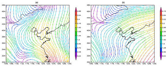
Figure 3.
1000 hpa (a) and 850 hpa (b) average wind patterns in summer.
3.2. Local Induced Enhancement of Precipitation and Urban Distribution
To reasonably determine the size of the moving window in MSP, the spatial autocorrelation of rainfall in different level years were estimated. As described in the previous section, the precipitation in the study area showed an obvious trend (from east to west and from south to north). Five different level years are identified from 1998–2018, where the normal year is 2003, the wet year and excessively wet year are 2004 and 2013, and the dry year and excessively dry year are 2000 and 2011. The summer precipitation anomaly percentage was calculated in every cell through the TRMM 3b43 monthly data. In this way, the trends can be eliminated. As shown in Figure 4, the precipitation anomaly percentage shows a positive spatial correlation until the distance is larger than 1.5 to 2.5 degrees. This suggests that when the distance between two rainfall cells is shorter, the yearly precipitation change tends to be more clearly synchronous. Thus, rainfall within 1.5 to 2.5 degrees could be considered impacted by the same local climate forcing factors. This paper set the size of the moving window in MSP as 1.75 degrees.
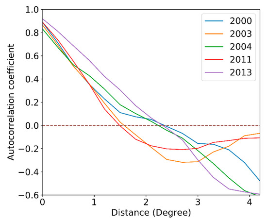
Figure 4.
Precipitation anomaly percentage spatial correlogram.
The MSP was performed, and the LIEP distribution is shown in Figure 5a. As shown in Figure 5a, for LIEP, the most obvious high value area is located downwind of Beijing-Tianjin-Tangshan. This location happens to be on the windward slope of the northern mountains, which overlaps considerably with the high loading area of the EOF2 mode of summer rainfall (Figure 2c). Meanwhile, Ref. [20] validated that the change of land use in Beijing-Tianjin-Tangshan practically led to an increase in rainfall volume and frequency in this area based on simulation by WRF coupled with the UCM model. Thus, the LIEP of this area should be influenced by both the terrain uplift and urbanization effects. According to the basin topography variation and urban distribution patterns, the areal LIEP distribution above the 500 m contour shows that the boundary of high and low LIEP is mostly concentrated in the zigzag part of the topographic contour but without an obvious relation to urban distribution. That means that precipitation here is mostly influenced by complex local terrain deformation. Even if urban impacts exist, they would be covered up by the counterparts precipitated by the terrain factor. In the plain area, however, where the elevation is below the 50 m contour, the terrain is flat. It can be seen that several important urban centers (such as Beijing, Tianjin, Tangshan, and Baoding city) and their surrounding areas show obviously low LIEP concentrations, which can be considered as a response to urbanization.
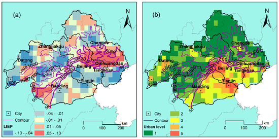
Figure 5.
Areal multi-year mean local induced enhancement of precipitation index (LIEP) (a) and urbanization level (b).
For the purpose of comparison with LIEP, the areal urbanization level distribution is provided in Figure 5b, where L1 to L5 represent the urbanization level from low to high. In this article, the urbanization level was derived from DMSP/OLS nightlight data, which were classified into five levels using the Jenks Natural Breaks method. Larger cities (areas with L4 or above and an extent larger than 2 cells) are mostly concentrated in the region below the 500m contour (the thick purple contour). Therefore, the spatial variation of precipitation caused by urbanization at the basin scale would mainly occur in the middle and downstream areas.
Statistical analysis was carried out on the LIEP in different urbanization level areas, and the boxplot result is shown in Figure 6. These results suggest that in the area where the urbanization level is high (L4 and L5), the summer LIEPs are relatively lower; even the upper quartile is less than zero. This means that the multi-year mean rainfall in a metropolis tends to be less than that in a peri-urban area. In the modest urbanization level (L3) areas located in the urban and rural junction zones, the LIEPs seem to be a bit larger, with a median greater than zero. However, the LIEPs in these areas show a larger deviation. In the rural area (L2, L1), the LIEP distribution is more even compared to the above areas.
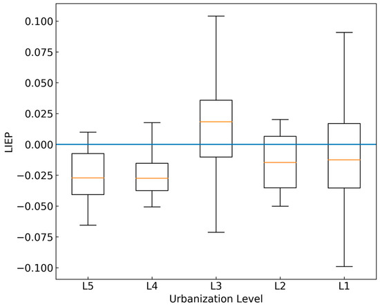
Figure 6.
The LIEP in different urbanization level areas.
3.3. Identifying the Precipitation Response to Urbanization
By using bivariate Moran’s I, LIEP was taken as the first variable, and URBI—represented by nighttime light data—was taken as the second variable for the spatial correlation analysis. The corresponding bivariate Moran’s I was estimated to be −0.11 (p < 0.001). This indicates that LIEP has a negative correlation with the surrounding area’s URBI. The LISA cluster map for LIEP and URBI is shown in Figure 7a.
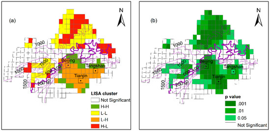
Figure 7.
Local indicators of spatial association (LISA) cluster (a) and significance (b) map for LIEP versus urban level.
The upstream region above the 500 m contour mainly features mountains and hills, with a low urban density and low urbanization level. Significant cluster types (significance level < 0.05, shown in Figure 7b) are defined as the high LIEP versus low URBI (H-L) and low LIEP versus low URBI (L-L), which suggests that the variance in LIEP is mainly influenced by the terrain factor, and the urban effects are obfuscated.
The middle and downstream region below the 500 m contour (the thick one) includes high urban density and a high urbanization level. The topography is a flat plain, thus, the terrain deformation effects can be excluded in the analysis of precipitation response. Significant cluster types (significance level < 0.05) consist of high LIEP versus High URBI (H-H) and Low LIEP versus High URBI (L-H). The inner parts of the city agglomeration show an L-H cluster, which suggests that highly urbanized areas induced a decrease of the summer precipitation compared to the surrounding areas. This result is consistent with the conclusions of [20] and [54]. The edge of the urban agglomeration shows significant H-H clustering, indicating that the suburban area can induce a certain increase in precipitation, which further confirms the results in Figure 6.
From the above, the LIEP of the region below the 500 m contour clumped in the L-H and H-H clusters embodies the influence caused by urban effects, with the terrain effects removed. Thus, the LIEP in these parts can be restated as the UIEP. In general, a bivariate Moran’s I for LIEP versus URBI coupled with DEM segmentation could effectively extract the urban agglomeration’s area of influence on precipitation form the north Haihe basin. Thus, these areas were taken as the ROI for the next analysis on the correlation between UIEP and potential influencing factors.
3.4. The Spatial Correlation between UIEP and URBI
It can be seen that the inner parts of ROI show a “dry island effect”, while the edge parts show a “wet island effect” (Figure 6 and Figure 7). Since the precipitation response to the urbanization level in different parts of the urban agglomeration might vary, the spatial non-stationarity of their relation needs to be investigated. For this purpose, a GWR model was established to analyze the spatial correlation between the multi-year averages of UIEP and URBI. The R2 and Akaike information criteria (AIC) are, respectively, 0.82 and −283.71. The estimated regression coefficients are shown as Figure 8. In the summer, “dry island effect” dominated inner parts, the estimated coefficients of URBI are negative but infinitesimal. This means that higher URBI may lead to a more remarkable “dry” condition but with a slight sensitivity. In the “wet island effects” dominated edge parts, where spots are marked with a red border, the estimated coefficients of URBI are still negative but larger. This indicates that the “wet island effect” is inhibited by the urbanization to some extent and is more sensitive to the URBI than the inner areas.
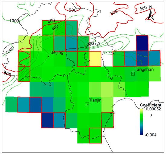
Figure 8.
The distribution of the estimated regression coefficient of urbanization index (UBRI). Squares outlined in red represent the “wet island effects” dominated area.
3.5. Lagged Correlation of UIEP and Climate Anomalies
As mentioned above, URBI has a significant impact on the spatial distribution of the multi-year average UIEP, but the varying strength of UIEP in each year is considered to be influenced by the climatic background [25]. The ROI area is located in the east Asian monsoon (EASM) area, and the summer precipitation is controlled by the EASM [55]. The UIEP is thus expected to be influenced by the EASM. Since the ENSO was considered to have a great impact on EASM (Hao and Ding 2012) [56], the potential association between UIEP and ENSO is worthy of studying. We calculated the 1–12-month lag correlation fields of UIEP versus Niño3.4 and SOI from 1998 to 2018. Given the space limitations, only 0–5-month lag correlation fields are shown in Figure 9 and Figure 10.
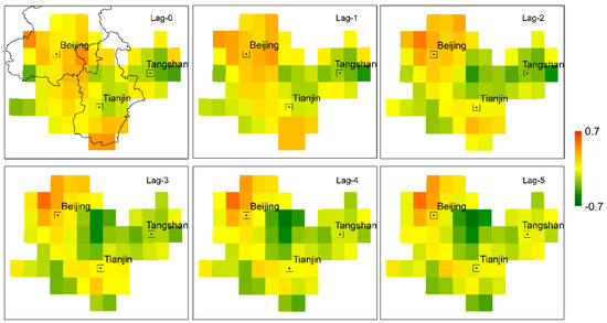
Figure 9.
0–5-month lag correlation fields between the urban induced enhancement of precipitation (UIEP) and Niño3.4 in the region of interest (ROI).
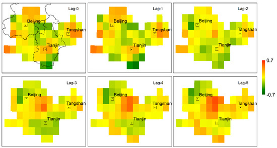
Figure 10.
0–5-month lag correlation fields between UIEP and Southern Oscillation Index (SOI) in ROI.
From Figure 9 and Figure 10, it can be seen that the regional UIEP shows spatial differentiation for a correlation with climate anomalies during 1998–2018. In Figure 9, the sites where the correlation between UIEP and Niño3.4 is strong appear frequently around the urban core area (marked as a square with a dot in the center), while in the urban core, this association is relatively weak. Among them, the junction zone of Beijing and Tianjin and northwest of Beijing show the most intensive correlation. As mentioned above, urbanization generally induced a “dry island” and a “wet island”, respectively, in the inner area and the edge part of the urban agglomeration from a multi-year average precipitation perspective. However, the pattern in which the UIEP is impacted by climate anomalies tends to be different. The highest urbanized core area, which is the low value center of UIEP, tends to be weakly related to Niño3.4, while the peri-urban-core area may have a stronger relation with Niño3.4, but the direction of this association is somewhat dependent on the position of the site. Overall, the performances of Niño3.4 and SOI have opposite effects on the UIEP strength of the coming summer. Jiang et al. (2019) reported the similar opposite effects of Niño3.4 and SOI on extreme precipitation indexes (EPIs) [57].
To judge the overall correlation between regional UIEP and climate factors, the spatial patterns and temporal coefficients of UIEP were isolated using the EOF method, and the temporal coefficient corresponding to the first mode (PC1) was taken to perform a correlation analysis with UIEP. For the 1–12-month lagged UIEP versus Niño3.4 and SOI, the analysis results show that the correlation between PC1 and Niño3.4 is largest when the lagged time of UIEP is 5 months, and the correlation between PC1 and SOI is largets when the lagged time of UIEP is 1 month.
3.6. Cross-Wavelet Analysis
The cross wavelet transform method (XWT) is further adopted to discuss the nonlinear correlation between the UIEP and climate anomalies, and the periodic characteristics are revealed from the perspective of multiple time scales. According to the EOF analysis results, the cross-wavelet spectrum of the first principal component (PC1) of UIEP against Niño3.4 and SOI is shown in Figure 11.
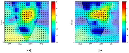
Figure 11.
The cross-wavelet spectrum of TS1 of the 5-month and 1-month lagged UIEP against Niño3.4 (a) and SOI (b). The thin black line represents the cone of influence. The thick enclosed areas denote the 5% significance level using red noise model based on Monte Carlo simulation method. Arrows signify the phase difference of oscillation. The arrow → means the in-phase relationship between the UIEP and climate anomalies, and ← means the anti-phase. The arrow ↓ means climate anomalies leading UIEP by 90°, and vice versa.
The significant sections shown in Figure 11 indicate a large covariance between both Niño3.4 and SOI against UIEP at a time scale of 2 years. The 5-month lagged UIEP versus Niño3.4 presents a significantly high common power period from 2007 to 2011, and Niño3.4 leads UIEP by about 135°. The 1-month lagged UIEP versus SOI shows significantly high common power periods from 2006 to 2012, while they are in the anti-phase.
3.7. Limitation and Uncertainties
Many studies have shown that precipitation response to urbanization has clear regional characteristics. At present, the statistical analysis of urban precipitation research based on measured surface station data inevitably yields certain uncertainties because of the spatial discontinuity of the data itself. However, spatially continuous high-resolution radar rainfall data or other emerging precipitation monitoring data (such as the data estimated using commercial microwave communication networks) [58,59] are difficult to access, and data series are always not long enough to meet the requirements of statistical analysis. Moreover, simulation studies on mesoscale climate models, such as WRF and MM5, generally lack long series simulations at inter-annual and inter-decadal scales. In this context, the data for satellite precipitation (e.g., TRMM) could provide data support for the statistical analysis of precipitation responses induced by urbanization precipitation. However, due to the characteristics of satellite precipitation products, the much more detailed precipitation distribution in urban areas is reflected coarsely, and these data have a poor ability to capture smaller cities at the basin scale.
Precipitation is an important component of the hydrology cycle. In the current research on hydrological responses to urbanization within a watershed, the hydrological model is the main means of research. However, how to present the impact of urbanization on various stages of the hydrologic process remains a challenge. Generally, hydrological models driven by limited observation station precipitation data are adopted to merely explore the influence caused by impervious surfaces to water yielding. In a basin where urban elements are well developed, if the influenced distribution of precipitation is neglected, urbanization effects are not considered comprehensively. Although this paper discussed the urban effects on precipitation in the north Haihe basin, the results here also describe regional characteristics. The universal regularity of the urban scale versus rainfall variation need to be further analyzed to yield any conclusions.
4. Conclusions
- By comparing the distribution of LIEP and the urban level, the urbanization effects on summer rainfall in the upstream mountainous area were found to be hidden away by topographic factors.
- From the basin perspective, the highest urbanization level areas have the lowest LIEP, while the suburban areas have the highest LIEP, and the rural areas are in the middle.
- LISA clustering for LIEP and URBI based on bivariate Moran’s I coupled with DEM segmentation could efficiently extract the urban influencing area. The precipitation response is different to URBI in different parts of ROI. The UIEP and the URBI are generally negatively correlated. Precipitation in the inner parts of the ROI is less sensitive to URBI, while precipitation in the edge area of the ROI part is more sensitive to the URBI.
- The low UIEP value centers that happen to be the urban core areas have a weak correlation with ENSO, while the UIEP in the peri-urban-core areas have a stronger correlation with ENSO. UIEP versus Niño3.4 and SOI both show a significant common high-power period at a time scale of 2 years.
Author Contributions
Conceptualization, R.C. and F.L.; methodology, R.C.; software, R.C.; validation, F.L., P.F.; formal analysis, R.C.; writing—original draft preparation, R.C.; writing—review and editing, R.C. and F.L.; funding acquisition, P.F. All authors have read and agreed to the published version of the manuscript.
Funding
This research was funded by the National Natural Science Foundation of China, grant number 51779165 and 51879181.
Conflicts of Interest
The authors declare no conflict of interest.
References
- Changnon, S.A. Rainfall Changes in Summer Caused by St. Louis. Science 1979, 205, 402–404. [Google Scholar] [CrossRef] [PubMed]
- Lei, M.; Niyogi, D.; Kishtawal, C.; Pielke, R.A.; Beltran-Przekurat, A.; Nobis, T.E.; Vaidya, S.S. Effect of explicit urban land surface representation on the simulation of the 26 July 2005 heavy rain event over Mumbai, India. Atmos. Chem. Phys. 2008, 8, 5975–5995. [Google Scholar] [CrossRef]
- Hu, Q.; Zhang, J.; Wang, Y.; Huang, Y.; Liu, Y.; Li, L. A review of urbanization impact on precipitation. Adv. Water Sci. 2018, 29, 138–150. [Google Scholar]
- Song, X.; Zhang, J.; AghaKouchak, A.; Roy, S.; Xuan, Y.; Wang, G.; He, R.; Wang, X.; Liu, C. Rapid urbanization and changes in spatiotemporal characteristics of precipitation in Beijing metropolitan area. J. Geophys. Res. Atmos. 2014, 119, 11250–11271. [Google Scholar] [CrossRef]
- Li, X.; Zhou, W.; Ouyang, Z. Forty years of urban expansion in Beijing: What is the relative importance of physical, socioeconomic, and neighborhood factors? Appl. Geogr. 2013, 38, 1–10. [Google Scholar] [CrossRef]
- Li, W.; Chen, S.; Chen, G.; Sha, W.; Luo, C.; Feng, Y.; Wen, Z.; Wang, B. Urbanization signatures in strong versus weak precipitation over the Pearl River Delta metropolitan regions of China. Environ. Res. Lett. 2011, 6, 034020. [Google Scholar] [CrossRef][Green Version]
- Wan, H.; Zhong, Z.; Yang, X.; Li, X. Impact of city belt in Yangtze River Delta in China on a precipitation process in summer: A case study. Atmos. Res. 2013, 125, 63–75. [Google Scholar] [CrossRef]
- Yu, M.; Miao, S.; Zhang, H. Uncertainties in the Impact of Urbanization on Heavy Rainfall: Case Study of a Rainfall Event in Beijing on 7 August 2015. J. Geophys. Res. Atmos. 2018, 123, 6005–6021. [Google Scholar] [CrossRef]
- Chen, X.; Liu, B.; Chen, G. Effects of Urbanization on Precipitation Characteristics. J. Nat. Resour. 2017, 32, 1591–1601. [Google Scholar]
- Zhu, X.; Zhang, Q.; Sun, P. Effects of urbanization on spatio-temporal distribution of precipitations in Beijing and its related causes. Acta Geogr. Sin. 2018, 73, 2086–2104. [Google Scholar]
- Shepherd, J.M.; Burian, S.J. Detection of Urban-Induced Rainfall Anomalies in a Major Coastal City. Earth Interact. 2003, 7, 1–17. [Google Scholar] [CrossRef]
- Mote, T.L.; Lacke, M.C.; Shepherd, J.M. Radar signatures of the urban effect on precipitation distribution: A case study for Atlanta, Georgia. Geophys. Res. Lett. 2007, 34, L20710. [Google Scholar] [CrossRef]
- Yan, Z.; Wang, J.; Xia, J.-J.; Feng, J. Review of recent studies of the climatic effects of urbanization in China. Adv. Clim. Chang. Res. 2016, 7, 154–168. [Google Scholar] [CrossRef]
- Li, J.; Zheng, X.; Zhang, C.; Chen, Y. Impact of Land-Use and Land-Cover Change on Meteorology in the Beijing-Tianjin-Hebei Region from 1990 to 2010. Sustainability 2018, 10, 176. [Google Scholar] [CrossRef]
- Wang, Y.; Sabatino, S.D.; Martilli, A.; Li, Y.; Wong, M.S.; Gutiérrez, E.; Chan, P.W. Impact of land surface heterogeneity on urban heat island circulation and sea-land breeze circulation in Hong Kong. J. Geophys. Res. Atmos. 2017, 122, 4332–4352. [Google Scholar] [CrossRef]
- Wai, K.M.; Wang, X.M.; Lin, T.H.; Wong, M.S.; Zeng, S.K.; He, N.; Ng, E.; Lau, K.; Wang, D.H. Observational evidence of a long-term increase in precipitation due to urbanization effects and its implications for sustainable urban living. Sci. Total Environ. 2017, 599, 647–654. [Google Scholar] [CrossRef]
- Salvadore, E.; Bronders, J.; Batelaan, O. Hydrological modelling of urbanized catchments: A review and future directions. J. Hydrol. 2015, 529, 62–81. [Google Scholar] [CrossRef]
- Debbage, N.; Shepherd, J.M. Urban Influences on the Spatiotemporal Characteristics of Runoff and Precipitation during the 2009 Atlanta Flood. J. Hydrometeorol. 2019, 20, 3–21. [Google Scholar] [CrossRef]
- McLeod, J.; Shepherd, M.; Konrad, C.E. Spatio-temporal rainfall patterns around Atlanta, Georgia and possible relationships to urban land cover. Urban Clim. 2017, 21, 27–42. [Google Scholar] [CrossRef]
- Zhang, S.; Huang, G.; Wang, J.; Liu, Y.; Jia, G.; Ren, G. Impact of Urban Surface Characteristics on Summer Rainfall in the Beijing-Tianjin-Hebei Area. Chinese J. Atmos. Sci. 2015, 39, 911–925. [Google Scholar]
- Li, S.; Ma, J. Impact of urbanization on precipitation in Beijing area. J. Meteorol. Sci. 2011, 31, 414–421. [Google Scholar]
- Yu, X.; Yang, G.; Zhou, Z.; Wang, J.; Qin, D. Variation of summer precipitation in Tianjin region and its urbanization effect. Prog. Geogr. 2008, 27, 43–48. [Google Scholar]
- Mitra, C.; Shepherd, J.M.; Jordan, T. On the relationship between the premonsoonal rainfall climatology and urban land cover dynamics in Kolkata city, India. Int. J. Climatol. 2012, 32, 1443–1454. [Google Scholar] [CrossRef]
- Li, W.; He, X.; Scaioni, M.; Yao, D.; Mi, C.; Zhao, J.; Chen, Y.; Zhang, K.; Gao, J.; Li, X. Annual precipitation and daily extreme precipitation distribution: Possible trends from 1960 to 2010 in urban areas of China. Geomat. Nat. Hazards Risk 2019, 10, 1694–1711. [Google Scholar] [CrossRef]
- Zhang, S.; Huang, G.; Qi, Y.; Jia, G. Impact of urbanization on summer rainfall in Beijing–Tianjin–Hebei metropolis under different climate backgrounds. Theor. Appl. Climatol. 2018, 133, 1093–1106. [Google Scholar] [CrossRef]
- Pachauri, R.K.; Mayer, L.; Intergovernmental Panel on Climate Change (Eds.) Climate Change 2014: Synthesis Report; Intergovernmental Panel on Climate Change: Geneva, Switzerland, 2015; ISBN 978-92-9169-143-2. [Google Scholar]
- Chu, J.T.; Xia, J.; Xu, C.-Y.; Singh, V.P. Statistical downscaling of daily mean temperature, pan evaporation and precipitation for climate change scenarios in Haihe River, China. Theor. Appl. Climatol. 2010, 99, 149–161. [Google Scholar] [CrossRef]
- Chang, C.; Feng, P.; Li, F.; Gao, Y. Long-term variation of water vapor content and precipitation in the Haihe river basin. J. Water Clim. Chang. 2015, 6, 341–351. [Google Scholar] [CrossRef]
- Wang, Z.; Luo, Y.; Liu, C.; Xia, J.; Zhang, M. Spatial and temporal variations of precipitation in Haihe River Basin, China: Six decades of measurements. Hydrol. Process. 2011, 25, 2916–2923. [Google Scholar] [CrossRef]
- Huffman, G.J.; Adler, R.F.; Bolvin, D.T.; Nelkin, E.J. The TRMM Multi-Satellite Precipitation Analysis (TMPA). In Satellite Rainfall Applications for Surface Hydrology; Gebremichael, M., Hossain, F., Eds.; Springer: Dordrecht, The Netherlands, 2010; pp. 3–22. ISBN 978-90-481-2915-7. [Google Scholar]
- Precipitation Measurement Missions | An international partnership to understand precipitation and its impact on humankind. Available online: https://pmm.nasa.gov/ (accessed on 20 November 2019).
- Geospatial Data Cloud. Available online: http://www.gscloud.cn/ (accessed on 20 November 2019).
- Earth Observation Group—Defense Meteorological Satellite Program, Boulder | ngdc.noaa.gov. Available online: https://www.ngdc.noaa.gov/eog/dmsp/downloadV4composites.html (accessed on 20 November 2019).
- Croft, T. Nighttime Images of the Earth from Space. Sci. Am. 1978, 239, 86–98. [Google Scholar] [CrossRef]
- Wang, L.; Li, W.; Wang, P.; Liu, X.; Yang, F.; Qu, J.J. Spatiotemporal characterization of the urban sprawl and its impacts on urban island in China with DMSP/OLS and MODIS measurements. Theor. Appl. Climatol. 2019, 138, 293–303. [Google Scholar] [CrossRef]
- Cong, Z.; Shen, Q.; Zhou, L.; Sun, T.; Liu, J. Evapotranspiration estimation considering anthropogenic heat based on remote sensing in urban area. Sci. China Earth Sci. 2017, 60, 659–671. [Google Scholar] [CrossRef]
- Wang, S.; Fang, C.; Sun, L.; Su, Y.; Chen, X.; Zhou, C.; Feng, K.; Hubacek, K. Decarbonizing China’s Urban Agglomerations. Ann. Am. Assoc. Geogr. 2019, 109, 266–285. [Google Scholar] [CrossRef]
- Wang, S.; Liu, X. China’s city-level energy-related CO2 emissions: Spatiotemporal patterns and driving forces. Appl. Energy 2017, 200, 204–214. [Google Scholar] [CrossRef]
- ESRL: PSD: PSD/Climate Diagnostics Branch, Data: NCEP Reanalysis Surface. Available online: https://www.esrl.noaa.gov/psd/data/gridded/data.ncep.reanalysis.surface.html (accessed on 20 November 2019).
- Peixoto, J.P.; Oort, A.H. Physics of Climate; AIP-Press: College Park, MD, USA, 1992; ISBN 978-0-88318-712-8. [Google Scholar]
- Kim, B.S.; Hossein, S.Z.; Choi, G. Evaluation of temporal-spatial precipitation variability and prediction using seasonal ARIMA model in Mongolia. KSCE J. Civ. Eng. 2011, 15, 917–925. [Google Scholar] [CrossRef]
- North, G.R.; Bell, T.L.; Cahalan, R.F.; Moeng, F.J. Sampling Errors in the Estimation of Empirical Orthogonal Functions. Mon. Weather Rev. 1982, 110, 699–706. [Google Scholar] [CrossRef]
- Kong, F.; Wang, Y.; Fang, J.; Lu, L. Spatial Pattern of Summer Extreme Precipitation and Its Response to Urbanization in China (1961–2010). Resour. Environ. Yangtze Basin 2018, 27, 996–1010. [Google Scholar]
- Zha, Y.; Ni, S.; Yang, S. An Effective Approach to Automatically Extract Urban Land-use from TM Imagery. J. Remote Sens. 2003, 7, 37–40. [Google Scholar]
- Greene, C.S.; Robinson, P.J.; Millward, A.A. Canopy of advantage: Who benefits most from city trees? J. Environ. Manag. 2018, 208, 24–35. [Google Scholar] [CrossRef]
- Anselin, L.; Syabri, I.; Smirnov, O. Visualizing multivariate spatial correlation with dynamically linked windows. In Proceedings of the New Tools for Spatial Data Analysis, Proceedings of the Specialist Meeting, Santa Barbara, CA, USA, 10–11 May 2002. [Google Scholar]
- Anselin, L.; Syabri, I.; Kho, Y. GeoDa: An Introduction to Spatial Data Analysis. In Handbook of Applied Spatial Analysis: Software Tools, Methods and Applications; Fischer, M.M., Getis, A., Eds.; Springer: Berlin/Heidelberg, Germany, 2010; pp. 73–89. ISBN 978-3-642-03647-7. [Google Scholar]
- GeoDa on Github. Available online: http://geodacenter.github.io/ (accessed on 20 November 2019).
- Fotheringham, A.S.; Charlton, M.E.; Brunsdon, C. Geographically Weighted Regression: A Natural Evolution of the Expansion Method for Spatial Data Analysis. Environ. Plan. A 1998, 30, 1905–1927. [Google Scholar] [CrossRef]
- Fotheringham, A.; Brunsdon, C.; Charlton, M. Geographically Weighted Regression: The Analysis of Spatially Varying Relationships; John Wiley & Sons: Hoboken, NJ, USA, 2002; Volume 13. [Google Scholar]
- Lu, B.; Charlton, M.; Harris, P.; Fotheringham, A.S. Geographically weighted regression with a non-Euclidean distance metric: A case study using hedonic house price data. Int. J. Geogr. Inf. Sci. 2014, 28, 660–681. [Google Scholar] [CrossRef]
- Akaike, H. Information Theory and an Extension of the Maximum Likelihood Principle. In Breakthroughs in Statistics: Foundations and Basic Theory; Kotz, S., Johnson, N.L., Eds.; Springer Series in Statistics; Springer: New York, NY, USA, 1992; pp. 610–624. ISBN 978-1-4612-0919-5. [Google Scholar]
- Mohammadi, F.; Fakheri Fard, A.; Ghorbani, M.A. Application of cross-wavelet–linear programming–Kalman filter and GIUH methods in rainfall–runoff modeling. Environ. Earth Sci. 2019, 78, 168. [Google Scholar] [CrossRef]
- Zhao, D.; Wu, J. Changes in urban-related precipitation in the summer over three city clusters in China. Theor. Appl. Climatol. 2018, 134, 83–93. [Google Scholar] [CrossRef]
- Huang, R.H.; Lei, G.U.; Yu-Hong, X.U.; Zhang, Q.L. Characteristics of the Interannual Variations of Onset and Advance of the East Asian Summer Monsoon and Their Associations with Thermal States of the Tropical Western Pacific. Chin. J. Atmos. Sci. 2005, 29, 20–36. [Google Scholar]
- Hao, L.; Ding, Y. Progress of Precipitation Research in North China. Prog. Geogr. 2012, 31, 593–601. [Google Scholar]
- Jiang, R.; Wang, Y.; Xie, J.; Zhao, Y.; Li, F.; Wang, X. Assessment of extreme precipitation events and their teleconnections to El Niño Southern Oscillation, a case study in the Wei River Basin of China. Atmos. Res. 2019, 218, 372–384. [Google Scholar] [CrossRef]
- Messer, H.; Zinevich, A.; Alpert, P. Environmental monitoring by wireless communication networks. Science 2006, 312, 713. [Google Scholar] [CrossRef]
- Zinevich, A.; Alpert, P.; Messer, H. Estimation of rainfall fields using commercial microwave communication networks of variable density. Adv. Water Resour. 2008, 31, 1470–1480. [Google Scholar] [CrossRef]
© 2019 by the authors. Licensee MDPI, Basel, Switzerland. This article is an open access article distributed under the terms and conditions of the Creative Commons Attribution (CC BY) license (http://creativecommons.org/licenses/by/4.0/).