The Climatology and Trend of Surface Wind Speed over Antarctica and the Southern Ocean and the Implication to Wind Energy Application


Abstract
1. Introduction
2. Methods
3. Results
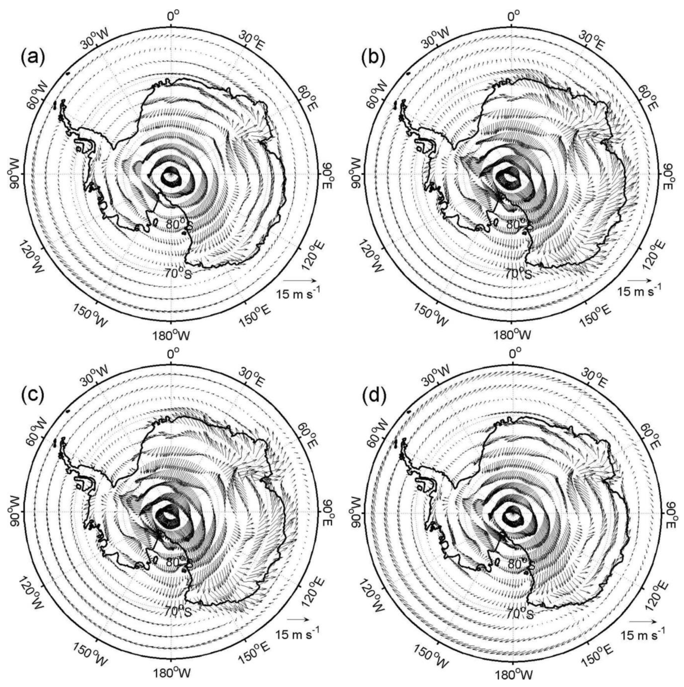
3.1. Annual and Interannual Variability
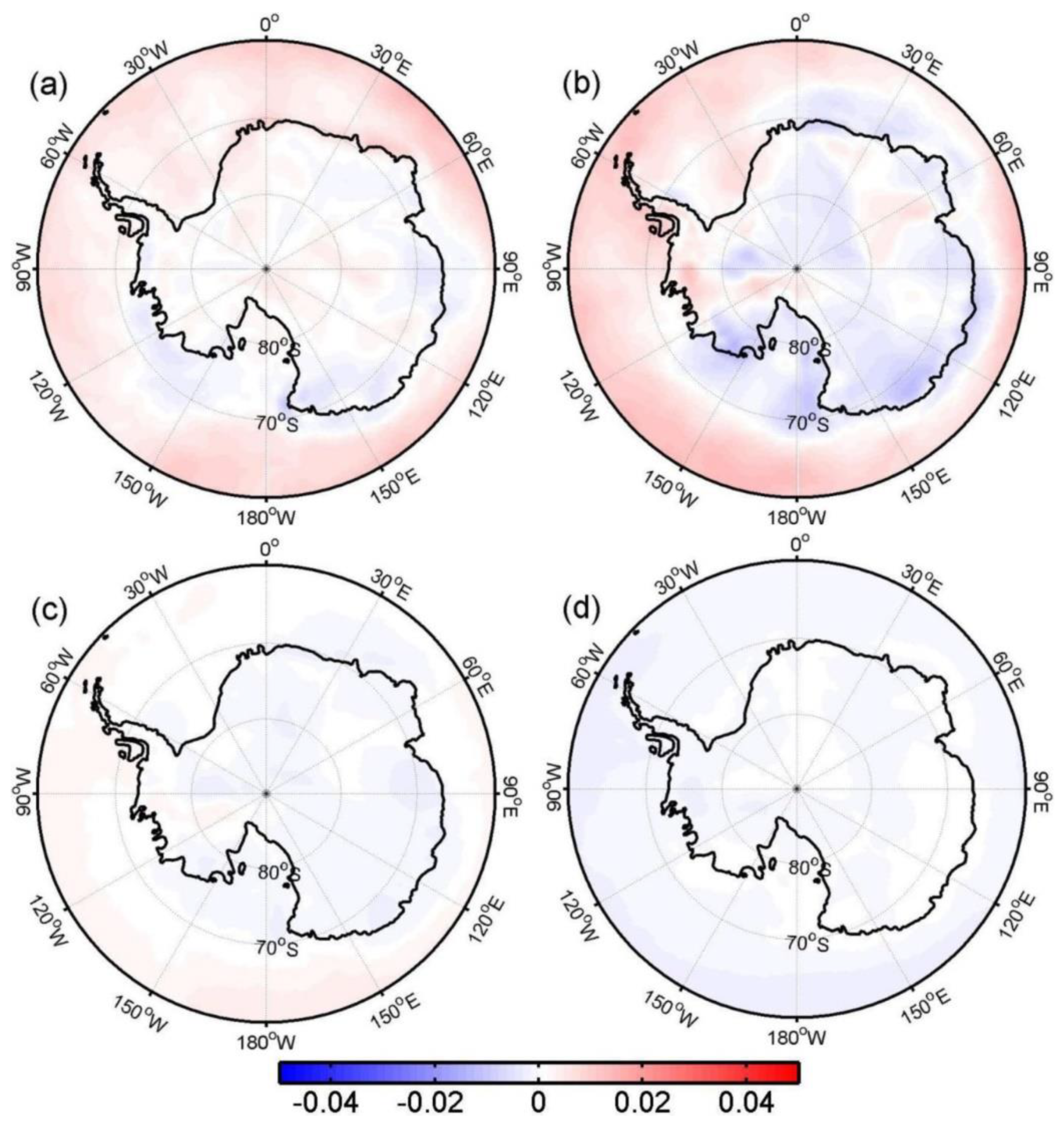
3.2. Trends
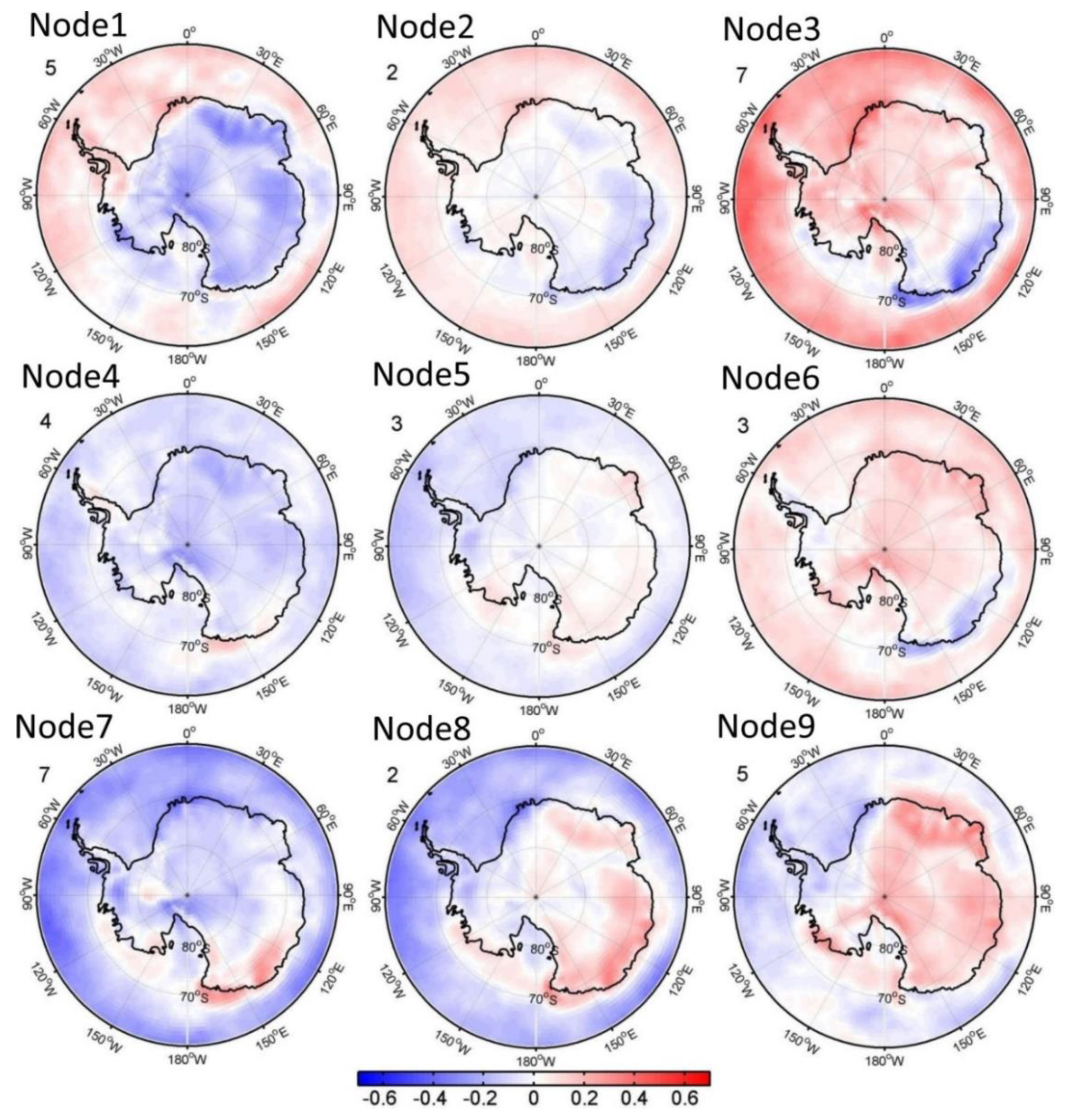
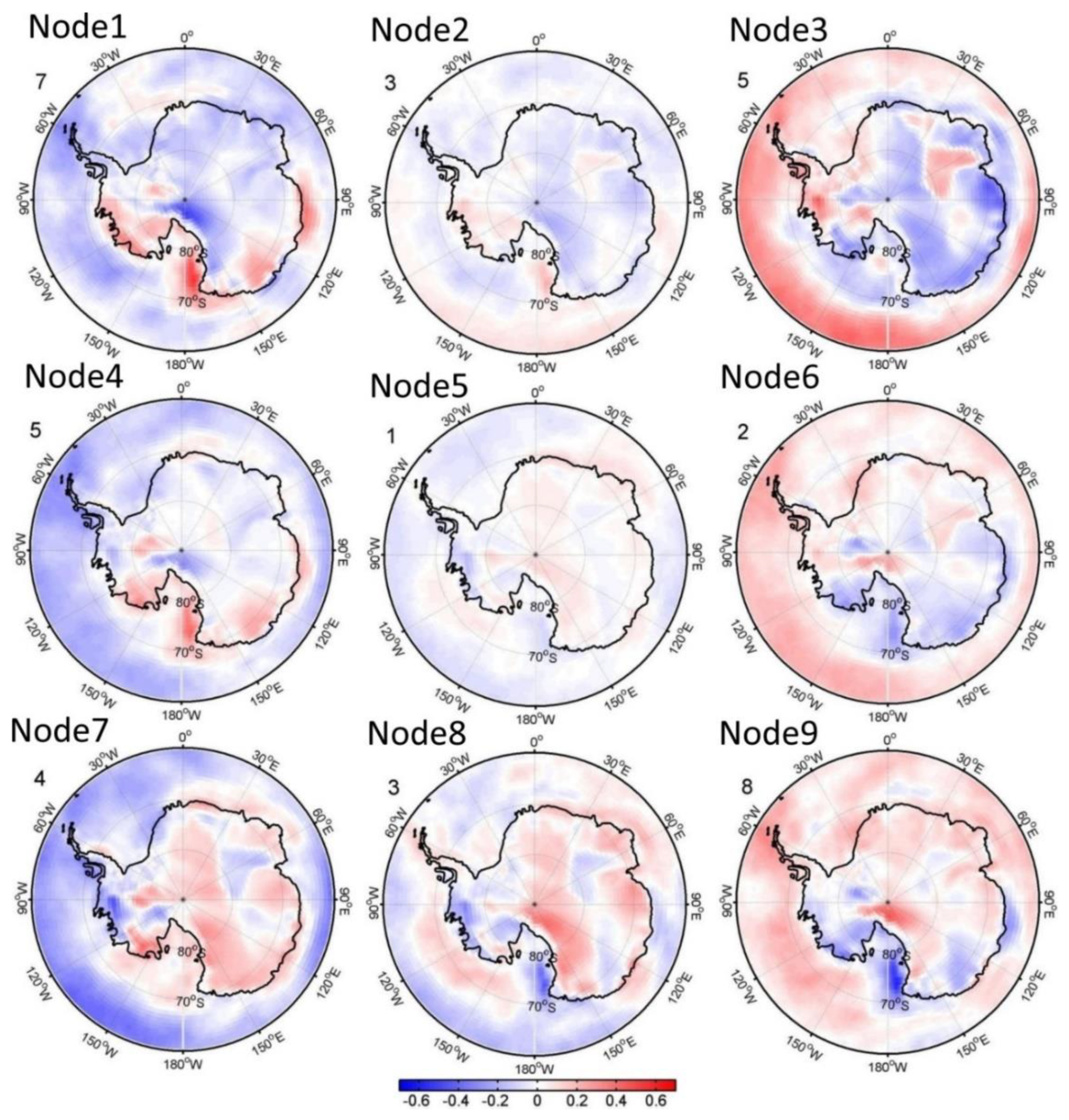
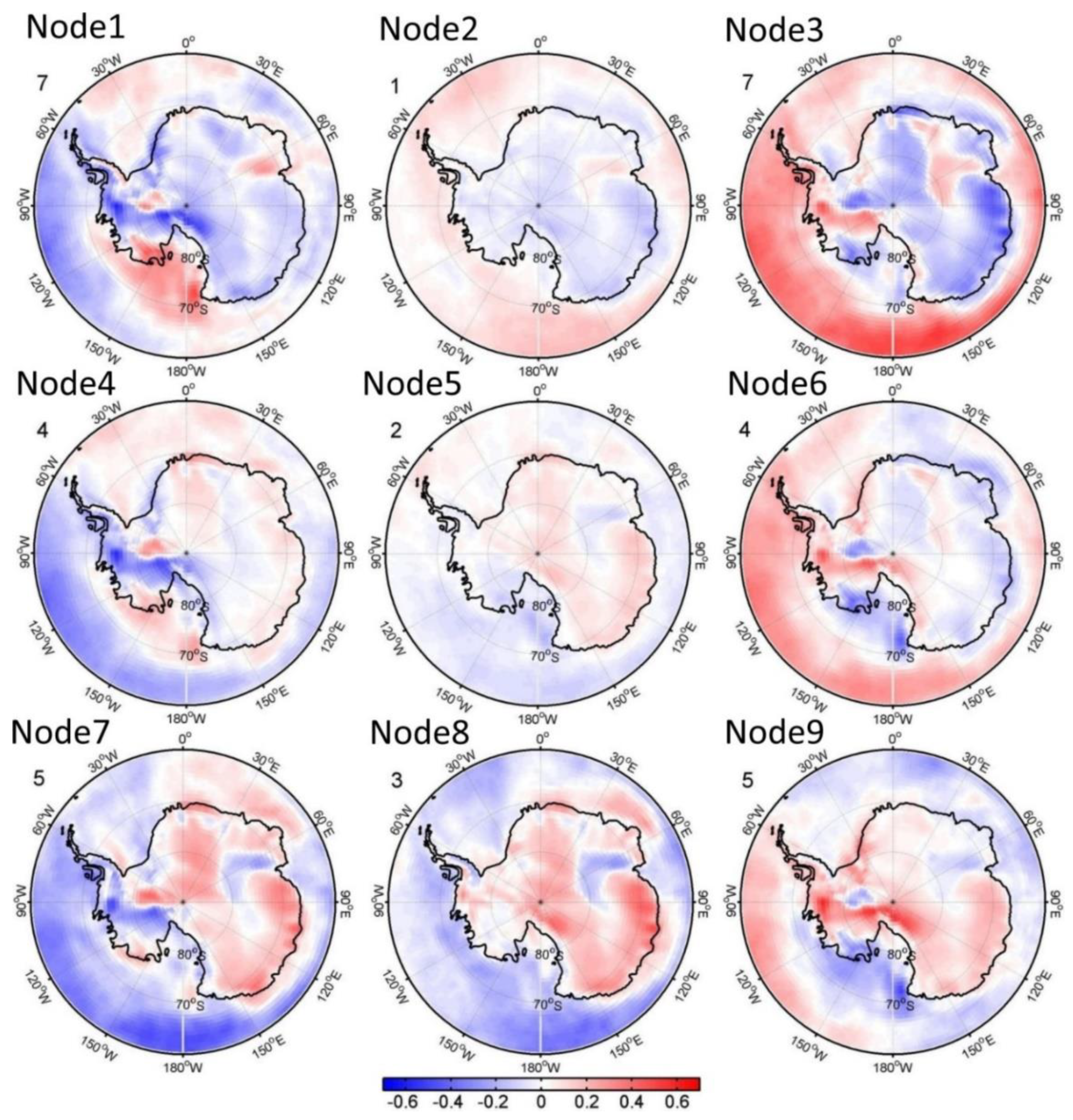
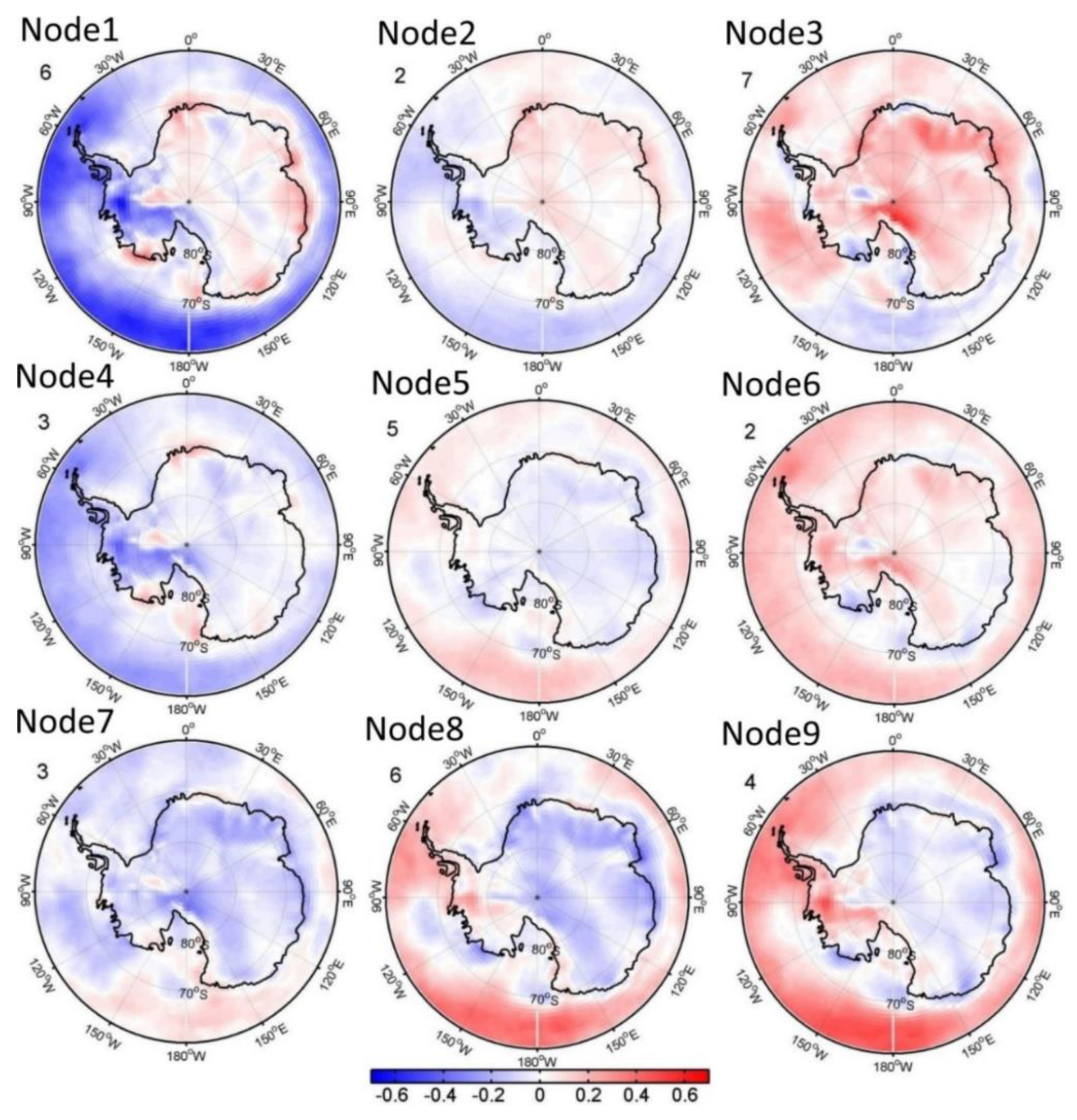
3.3. SOM Results
3.4. Wind Power Potential
4. Discussion and Conclusions
Author Contributions
Funding
Conflicts of Interest
References
- Czisch, G.; Ernst, B. High Wind Power Penetration by the Systematic Use of Smoothing Effects within Huge Catchment Areas Shown in a European Example. In Wind Power 2001; American Wind Energy Association: Washington, DC, USA, 2001. [Google Scholar]
- Archer, C.L.; Jacobson, M.Z. Spatial and temporal distributions of U.S. winds and wind power at 80 m derived from measurements. J. Geophys. Res. 2003, 108, 4289. [Google Scholar] [CrossRef]
- McVicar, T.R.; Van Niel, T.G.; Li, M.L.; Roderick, M.L.; Rayner, D.P.; Ricciardulli, L.; Donohue, R.J. Wind speed climatology and trends for Australia, 1975–2008: Capturing the stilling phenomenon and comparison with near-surface reanalysis output. Geophys. Res. Lett. 2008, 35, L20403. [Google Scholar] [CrossRef]
- Madhu, S.; Payal, S. A review of wind energy scenario in India. Int. Res. J. Environ. Sci. 2014, 3, 87–92. [Google Scholar]
- Yu, L.; Zhong, S.; Bian, X.; Heilman, W.E. Climatology and trend of wind power resources in China and its surrounding regions: A revisit using Climate Forecast System Reanalysis data. Int. J. Climatol. 2016, 36, 2173–2188. [Google Scholar] [CrossRef]
- Yu, L.; Zhong, S.; Zhou, M.; Sun, B.; Lenschow, D.H. Antarctic summer sea ice trend in the context of high-latitude atmospheric circulation changes. J. Clim. 2018, 31, 3909–3920. [Google Scholar] [CrossRef]
- Lu, X.; McElroy, M.B.; Kiviluoma, J. Global potential for wind-generated electricity. Proc. Natl. Acad. Sci. USA 2009, 106, 10933–10938. [Google Scholar] [CrossRef]
- Capps, S.B.; Zender, C.S. Estimated global ocean wind power potential from QuikSCAT observations, accounting for turbine characteristics and sitting. J. Geophys. Res. 2010, 115, D09101. [Google Scholar] [CrossRef]
- Zheng, C.W.; Pan, J. Assessment of the global ocean wind energy resource. Renew. Sustain. Energy Rev. 2014, 33, 382–391. [Google Scholar] [CrossRef]
- King, J.C.; Turner, J. Antarctic Meteorology and Climatology, 1st ed.; Cambridge University Press: Cambridge, UK, 1997; 409p. [Google Scholar]
- Guichard, A.; Magill, P.; Godon, P.; Lyons, D.; Brown, C. Potential for significant wind power generation at Antarctic stations. In Proceedings of the Seventh Symposium on Antarctic and Logistics Operation (SCALOP), Cambridge, UK, 6–7 August 1996. [Google Scholar]
- Ramesh, M.P. Wind Energy Applications in Indian Antarctic Station Maitri, Antarctica. In Sixteenth Indian Expedition to Antarctica; Scientific Report; Technical Publication No. 14; Department of Ocean Development: New Delhi, India, 2000; pp. 1–36. [Google Scholar]
- Teetz, H.W.; Harms, T.M.; von Backström, T.W. Assessment of the wind power potential at SANAE IV base, Antarctica: A technical and economic feasibility study. Renew. Energy 2003, 28, 2037–2061. [Google Scholar] [CrossRef]
- Lindquist, A. Wind Power in Antarctica-a Feasibility Study for Wasa. Master’s Thesis, Royal Swedish Academy of Sciences, Stockholm, Sweden, 2004. [Google Scholar]
- Rodrigo, J.S.; van Beeck, J.; Gorle, C.; Berte, J.; Dewilde, L.; Cabooter, Y.; Pattyn, F. Wind power in the future Belgian Antarctic research station. In Proceedings of the European Wind Energy Conference and Exhibition, Athens, Greece, 27 February 2006. [Google Scholar]
- Mather, K.B.; Miller, J.S. Wind drainage off the high plateau of eastern Antarctica. Nature 1966, 209, 281–284. [Google Scholar] [CrossRef]
- Parish, T.R. Surface airflow over East Antarctica. Mon. Weather Rev. 1982, 110, 84–90. [Google Scholar] [CrossRef]
- Parish, T.R.; Bromwich, D.H. The inversion wind pattern over West Antarctica. Mon. Weather Rev. 1986, 114, 849–860. [Google Scholar] [CrossRef]
- Parish, T.R.; Bromwich, D.H. The surface wind field over the Antarctic ice sheet. Nature 1987, 328, 51–54. [Google Scholar] [CrossRef]
- Parish, T.R.; Waight, K.T. The forcing of Antarctic katabatic winds. Mon. Weather Rev. 1987, 115, 2214–2226. [Google Scholar] [CrossRef]
- Gallée, J.; Schayes, G. Development of a three-dimensional Meso-γ primitive equation model: Katabatic winds simulation in the area of Terra Nova Bay, Antarctica. Mon. Weather Rev. 1994, 122, 671–685. [Google Scholar] [CrossRef]
- Van Lipzig, N.P.M.; van Meijgaard, E.; Oerlemans, J. Evaluation of a regional atmospheric model using measurements of surface heat exchange processes from a site in Antarctica. Mon. Weather Rev. 1994, 127, 11994–12011. [Google Scholar] [CrossRef]
- Hines, K.M.; Bromwich, D.H.; Parish, T.R. A mesoscale modeling study of the atmospheric circulation of high southern latitudes. Mon. Weather Rev. 1995, 123, 1146–1165. [Google Scholar] [CrossRef]
- Heinemann, G. Idealized simulations of the Antarctic katabatic wind system with a three-dimensional mesoscale model. J. Geophys. Res. 1997, 102, 13825–13834. [Google Scholar] [CrossRef]
- Bromwich, D.H.; Cassano, J.J.; Klein, T.; Heinemann, G.; Hines, K.M.; Steffen, K.; Box, J.E. Mesoscale modeling of katabatic winds over Greenland with the Polar MM5. Mon. Weather Rev. 2001, 129, 2290–2309. [Google Scholar] [CrossRef]
- Powers, J.G.; Monaghan, A.J.; Cayette, A.M.; Bromwich, D.H.; Kuo, Y.-H.; Manning, K.W. Real-time mesoscale modeling over Antarctica: The Antarctic mesoscale prediction system. Bull. Am. Meteorol. Soc. 2003, 84, 1533–1545. [Google Scholar] [CrossRef]
- Rodrigo, J.S.; Buchlin, J.M.; van Beeck, J.; Lenaerts, J.T.M.; van den Broeke, M.R. Evaluation of the Antarctic surface wind climate from ERA reanalyses and RACMO2/ANT simulations based on automatic weather stations. Clim. Dyn. 2013, 40, 353–376. [Google Scholar] [CrossRef]
- Bintanja, R.; Severijns, C.; Haarsma, R.; Hazeleger, W. The future of Antarctica’s surface winds simulated by a high-resolution global climate model: I. Model description and validation. J. Geophys. Res. 2014, 119, 7136–7159. [Google Scholar] [CrossRef]
- Parish, T.R. Surface winds over the Antarctic continent: A review. Rev. Geophys. 1988, 26, 169–180. [Google Scholar] [CrossRef]
- Van den Broeke, M.R.; van Lipzig, N.P.M. Factors controlling the near-surface wind field in Antarctica. Mon. Weather Rev. 2003, 131, 733–743. [Google Scholar] [CrossRef]
- Parish, T.R.; Cassano, J.J. Diagnosis of the katabatic wind influence on the wintertime antarctic surface wind field from numerical simulations. Mon. Weather Rev. 2003, 131, 1128–1139. [Google Scholar] [CrossRef]
- Yasunari, T.; Kodama, S. Intraseasonal variability of katabatic wind over East Antarctica and planetary flow regime in the Southern Hemisphere. J. Geophys. Res. 1993, 98, 13063–13070. [Google Scholar] [CrossRef]
- Simmonds, I.; Law, R. Associations between Antarctic katabatic flow and the upper level winter vortex. Int. J. Climatol. 1995, 15, 403–421. [Google Scholar] [CrossRef]
- Parish, T.R.; Bromwich, D.H. Reexamination of the near-surface airflow over the Antarctic continent and implications on atmospheric circulations at high southern latitudes. Mon. Weather Rev. 2007, 135, 1961–1973. [Google Scholar] [CrossRef]
- Turner, J.; Colwell, S.R.; Marshall, G.J.; Lachlan-Cope, T.; Carleton, A.M.; Jones, P.D.; Lagun, V.E.; Reid, P.A.; Iagovkina, S. Antarctic climate change during the last 50 years. Int. J. Climatol. 2005, 25, 279–294. [Google Scholar] [CrossRef]
- Turner, J.; Chenoli, S.N.; Samah, A.A.; Marshall, G.; Philips, T.; Orr, A. Strong wind events in the Antarctic. J. Geophys. Res. 2009, 114, D18103. [Google Scholar] [CrossRef]
- Chenoli, S.N.; Turner, J.; Samah, A.A. A climatology of strong wind events at McMurdo station, Antarctica. Int. J. Climatol. 2013, 33, 2667–2681. [Google Scholar] [CrossRef]
- Dee, D.P.; Uppala, S.M.; Simmons, A.J.; Berrisford, P.; Poli, P.; Kobayashi, S.; Andrae, U.; Balmaseda, M.A.; Balsamo, G.; Bauer, P.; et al. The ERA-Interim reanalysis: Configuration and performance of the data assimilation system. Q. J. R. Meteorol. Soc. 2011, 137, 553–597. [Google Scholar] [CrossRef]
- Bromwich, D.H.; Nicolas, J.P.; Monaghan, A.J. An assessment of precipitation changes over Antarctica and the Southern Ocean since 1989 in contemporary global reanalyses. J. Clim. 2011, 24, 4189–4209. [Google Scholar] [CrossRef]
- Klöwer, M.; Jung, T.; König-Langlo, G.; Semmler, T. Aspects of weather parameters at Neumayer station, Antarctica, and their representation in reanalysis and climate model data. Meteorol. Z. 2013, 22, 699–709. [Google Scholar] [CrossRef]
- Kohonen, T. Self-Organizing Maps; Springer: Berlin/Heidelberg, Germany, 2001; 501p. [Google Scholar]
- Sammon, J.W. A non-linear mapping for data structure analysis. IEEE Trans. Comput. 1969, 18, 401–409. [Google Scholar] [CrossRef]
- Reusch, D.B.; Alley, R.B.; Hewitson, B.C. Relative performance of self-organizing maps and principal component analysis in pattern extraction from synthetic climatological data. Polar Geogr. 2005, 29, 188–212. [Google Scholar] [CrossRef]
- Nigro, M.A.; Cassano, J.J. Identification of surface wind patterns over the Ross Ice Shelf, Antarctica, using self-organizing maps. Mon. Weather Rev. 2014, 142, 2361–2378. [Google Scholar] [CrossRef]
- Johnson, N.C. How many ENSO flavors can we distinguish? J. Clim. 2013, 26, 4816–4827. [Google Scholar] [CrossRef]
- Jones, D.A.; Simmonds, I. A climatology of Southern Hemisphere extratropical Cyclones. Clim. Dyn. 1993, 9, 131–145. [Google Scholar] [CrossRef]
- Kodama, Y.; Wendler, G. Wind and temperature regima along the slope of Adélie Land, Antarctica. J. Geophys. Res. 1986, 91, 6735–6741. [Google Scholar] [CrossRef]
- Carleton, A.M. A synoptic climatology of satellite-observed extratropical cyclones activity for the Southern Hemisphere winter. Arch. Meteorol. Geophys. Bioklimatol. 1979, 27, 265–279. [Google Scholar] [CrossRef]
- Thompson, D.W.J.; Wallace, J.M. Annular modes in the extratropical circulation. Part I: Month-to-month variability. J. Clim. 2000, 13, 1000–1016. [Google Scholar] [CrossRef]
- Mends, D.; Souza, E.P.; Marengo, J.A.; Mendes, M.C.D. Climatology of extratropical cyclones over the South American-southern oceans sector. Theor. Appl. Climatol. 2010, 100, 239–250. [Google Scholar] [CrossRef]
- Pezza, A.B.; Durrant, T.; Simmonds, I.; Smith, I. Southern hemisphere synoptic behavior in extreme phases of SAM, ENSO, sea ice extent, and Southern Australia rainfall. J. Clim. 2008, 21, 5566–5584. [Google Scholar] [CrossRef]
- Eichler, T.P.; Gottschalck, J. A comparison of southern hemisphere cyclone track climatology and interannual variability in coarse-gridded reanalysis datasets. Adv. Meteorol. 2013, 2013, 891260. [Google Scholar] [CrossRef]
- Simmonds, I. Comparing and contrasting the behavior of Arctic and Antarctic sea ice cover the 35 year period 1979-2013. Annu. Glaciol. 2015, 56, 18–28. [Google Scholar] [CrossRef]
- Wallenius, T.; Lehtomäki, V. Overview of cold climate wind energy: Challenges, solutions, and future needs. Wires Energy Environ. 2016, 5, 128–135. [Google Scholar] [CrossRef]
- Lacroix, A.; Manwell, J.F. Wind Energy: Cold Weather Issues; University of Massachusetts at Amherst, Renewable Energy Laboratory: Golden, CO, USA, 2000. [Google Scholar]
- Barristi, L. Wind Turbines in Cold Climates: Icing impacts and mitigation system. In Green Energy and Technology; Springer International Publishing: Cham, Switzerland, 2015; p. 333. [Google Scholar]
- Parish, T.R. The influence of the Antarctic Peninsula on the wind field over the western Weddell Sea. J. Geophys. Res. 1983, 88, 2684–2692. [Google Scholar] [CrossRef]
- Steinhoff, D.F.; Chaudhuri, S.; Bromwich, D.H. A case study of a Ross Ice Shelf air stream event: A new perspective. Mon. Weather Rev. 2009, 137, 4030–4046. [Google Scholar] [CrossRef]
- Pettré, P.; Payan, C.; Parish, T.R. Interaction of katabatic flow with local thermal effects in a coastal region of Adélie Land, East Antarctica. J. Geophys. Res. 1993, 98, 10429–10440. [Google Scholar] [CrossRef]
- Simmonds, I. Modes of atmospheric variability over the Southern Ocean. J. Geophys. Res. 2003, 108, 8078. [Google Scholar] [CrossRef]
- Matthewman, N.J.; Magnusdottir, G. Clarifying ambiguity in intraseasonal Southern Hemisphere climate modes during austral winter. J. Geophys. Res. 2012, 117, D03105. [Google Scholar] [CrossRef]
- Liess, S.; Kumar, A.; Snyder, P.K.; Kawale, J.; Steinhaeuser, K.; Semazzi, F.H.M.; Ganguly, A.R.; Samatova, N.F.; Kumar, V. Different modes of variability over the Tasman Sea: Implications for regional climate. J. Clim. 2014, 27, 8466–8486. [Google Scholar] [CrossRef]


| Regions | Summer (DJF) | Autumn (MAM) | Winter (JJA) | Spring (SON) |
|---|---|---|---|---|
| East Antarctica | 0.16 | −0.29 | −0.51 * | −0.02 |
| West Antarctica | 0.16 | −0.00 | −0.09 | 0.40 |
| Indian Ocean | 0.53 * | 0.27 | 0.19 | 0.36 * |
| Atlantic Ocean | 0.44 * | 0.71 * | 0.47 * | 0.55 * |
| Pacific Ocean | 0.39 * | 0.62 * | 0.58 * | 0.62 * |
| Whole region | 0.37 * | 0.29 | 0.06 | 0.45 * |
| Regions | Summer (DJF) | Autumn (MAM) | Winter (JJA) | Spring (SON) |
|---|---|---|---|---|
| East Antarctica | 0.0108 | 0.0023 | 0.0052 | 0.0115 |
| West Antarctica | 0.0100 | 0.0000 | −0.0020 | 0.0079 |
| Indian Ocean | 0.0130 | 0.0067 | 0.0126 | 0.0048 |
| Atlantic Ocean | 0.0119 | 0.0059 | 0.0073 | 0.0079 |
| Pacific Ocean | 0.0069 | 0.0021 | 0.0014 | −0.0026 |
| The whole region | 0.0101 | 0.0024 | 0.0035 | 0.0070 |
| Node1 | Node2 | Node3 | Node4 | Node5 | Node6 | Node7 | Node8 | Node9 | |
|---|---|---|---|---|---|---|---|---|---|
| Summer | −0.0032 | −0.0002 | 0.0117 * | −0.0050 | −0.0003 | 0.0093 * | −0.0156 * | −0.0002 | 0.0036 |
| (DJF) | 2.9% | 0.0% | 11.4% | 4.3% | 0.0% | 8.2% | 13.5% | 0.0% | 3.0% |
| Autumn | −0.0050 | −0.0071 | 0.0023 | −0.0115 * | 0.0012 | 0.0063 | −0.0037 | 0.0032 | 0.0098 * |
| (MAM) | 3/8% | 1.9% | 0.5% | 8.2% | 0.1% | 3.1% | 1.4% | 1.5% | 8.2% |
| Winter | −0.0045 | 0.0001 | −0.0034 | 0.0072 | 0.0020 | −0.0009 | −0.0003 | 0.0010 | −0.0012 |
| (JJA) | 0.6% | 0.0% | 0.5% | 1.2% | 0.3% | 0.0% | 0.0% | 0.2% | 0.0% |
| Spring | 0.0066 | −0.0050 | 0.0198 * | 0.0010 | −0.0056 | 0.0002 | −0.0086 * | −0.0083 | 0.0001 |
| (SON) | 1.3% | −2.2% | 27.9% | −0.4% | 2.0% | 0.1% | 8.7% | 8.1% | −0.0% |
© 2020 by the authors. Licensee MDPI, Basel, Switzerland. This article is an open access article distributed under the terms and conditions of the Creative Commons Attribution (CC BY) license (http://creativecommons.org/licenses/by/4.0/).
Share and Cite
Yu, L.; Zhong, S.; Sun, B. The Climatology and Trend of Surface Wind Speed over Antarctica and the Southern Ocean and the Implication to Wind Energy Application. Atmosphere 2020, 11, 108. https://doi.org/10.3390/atmos11010108
Yu L, Zhong S, Sun B. The Climatology and Trend of Surface Wind Speed over Antarctica and the Southern Ocean and the Implication to Wind Energy Application. Atmosphere. 2020; 11(1):108. https://doi.org/10.3390/atmos11010108
Chicago/Turabian StyleYu, Lejiang, Shiyuan Zhong, and Bo Sun. 2020. "The Climatology and Trend of Surface Wind Speed over Antarctica and the Southern Ocean and the Implication to Wind Energy Application" Atmosphere 11, no. 1: 108. https://doi.org/10.3390/atmos11010108
APA StyleYu, L., Zhong, S., & Sun, B. (2020). The Climatology and Trend of Surface Wind Speed over Antarctica and the Southern Ocean and the Implication to Wind Energy Application. Atmosphere, 11(1), 108. https://doi.org/10.3390/atmos11010108