Characteristics of Surface Ozone in Five Provincial Capital Cities of China during 2014–2015


 ,
, 
Abstract
1. Introduction
2. Methods and Data
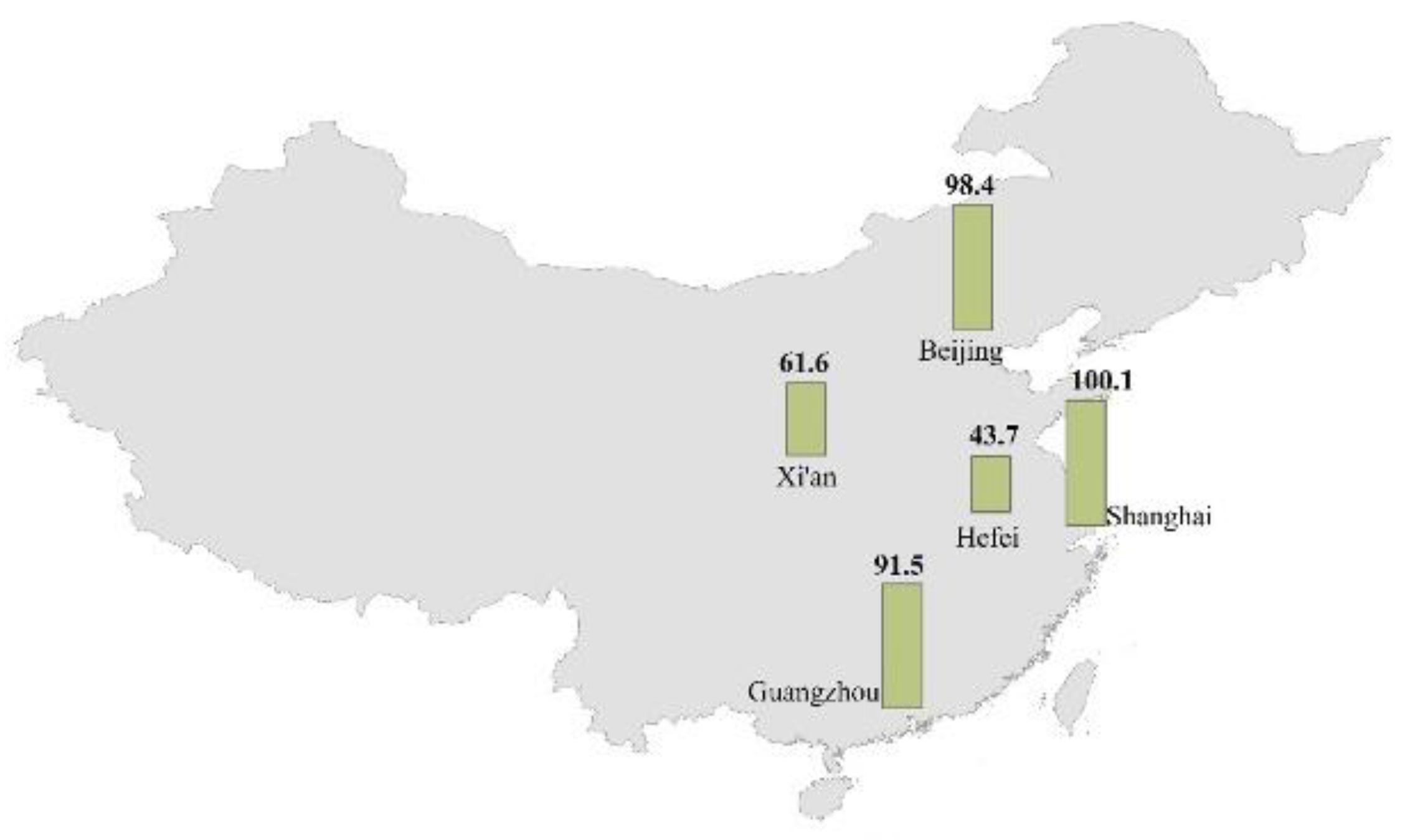
2.1. Study Cities
2.2. Data Collection
2.3. Back Trajectory Analysis
3. Results and Discussion
3.1. Overview of MDA8 O3 Levels
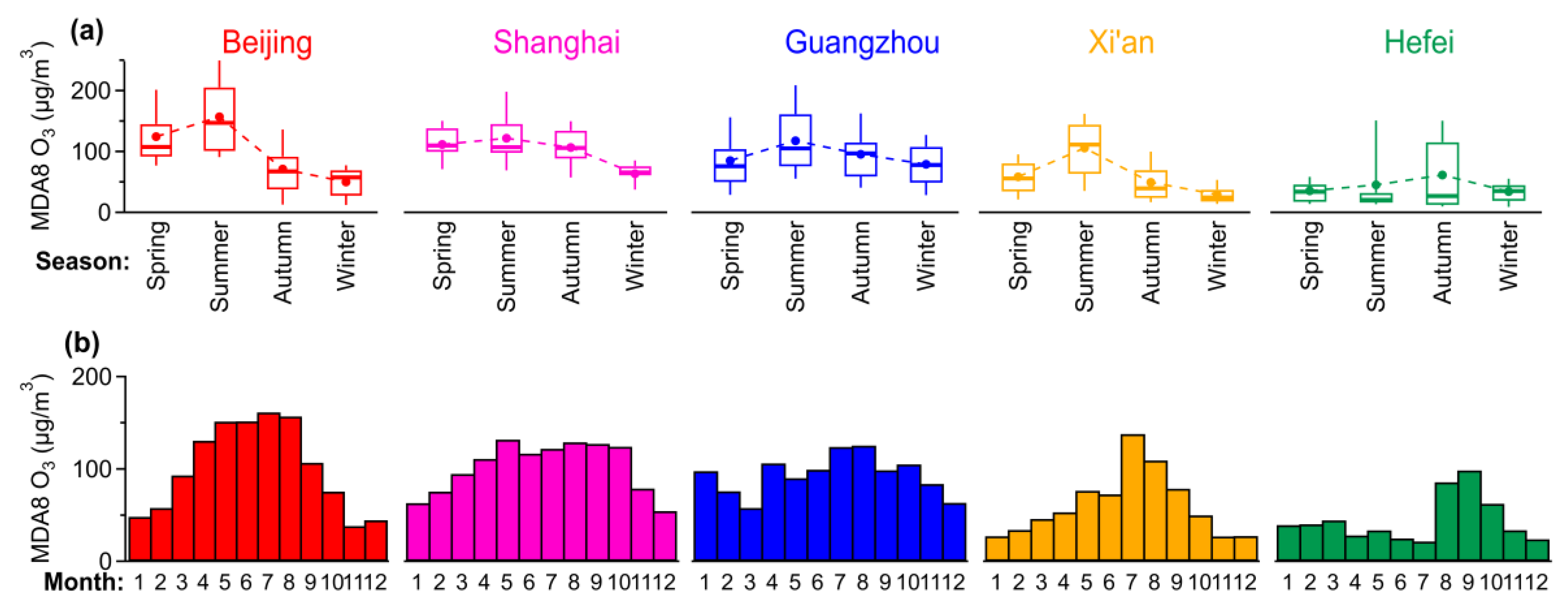
3.2. Seasonal and Monthly Variation
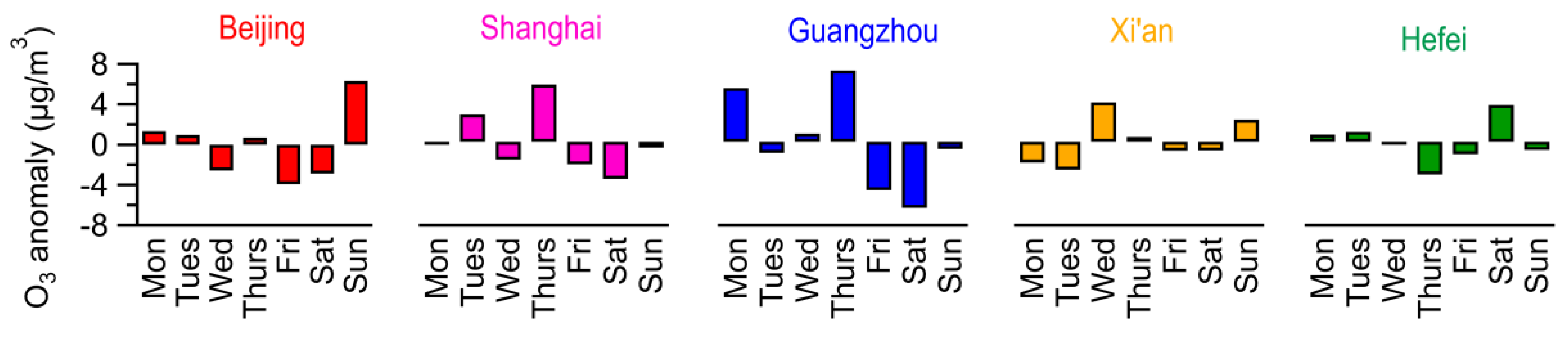
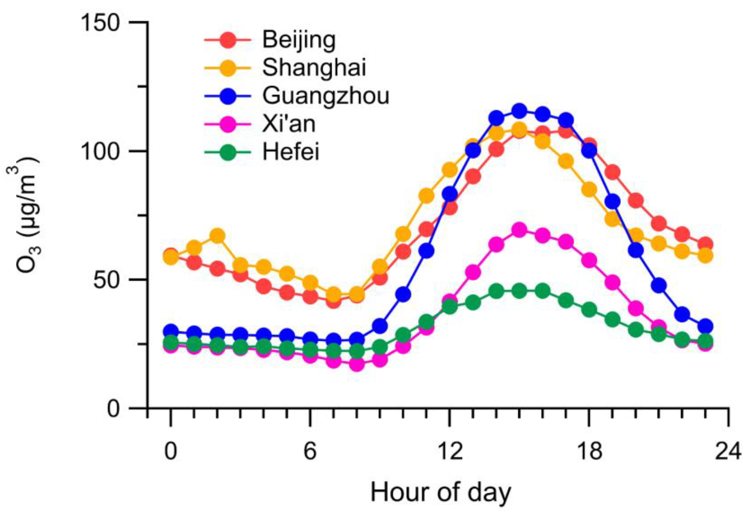
3.3. Weekly and Diurnal Patterns
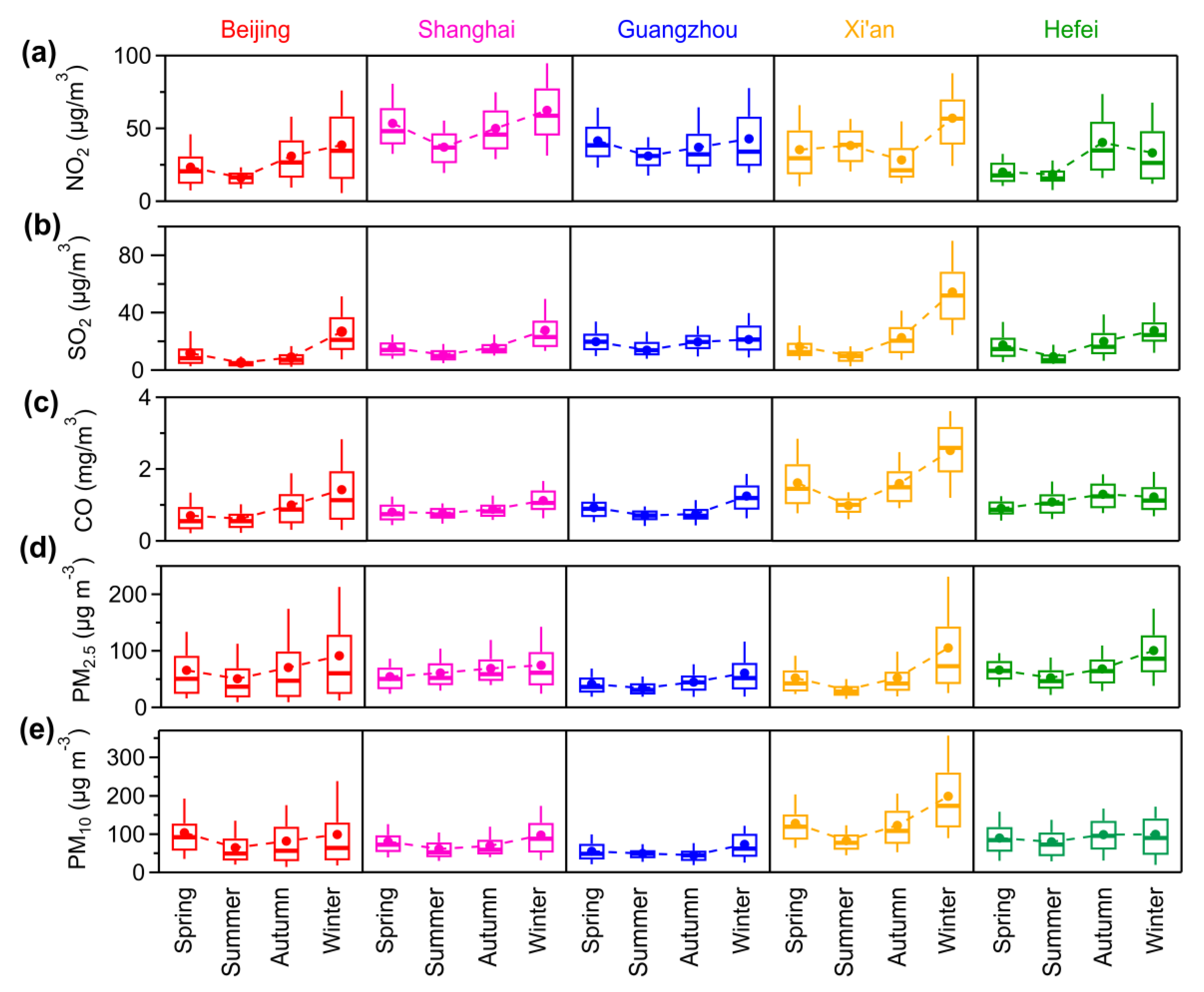
3.4. Effects of Air Pollutants and Meteorological Parameters on MDA8 O3 Levels
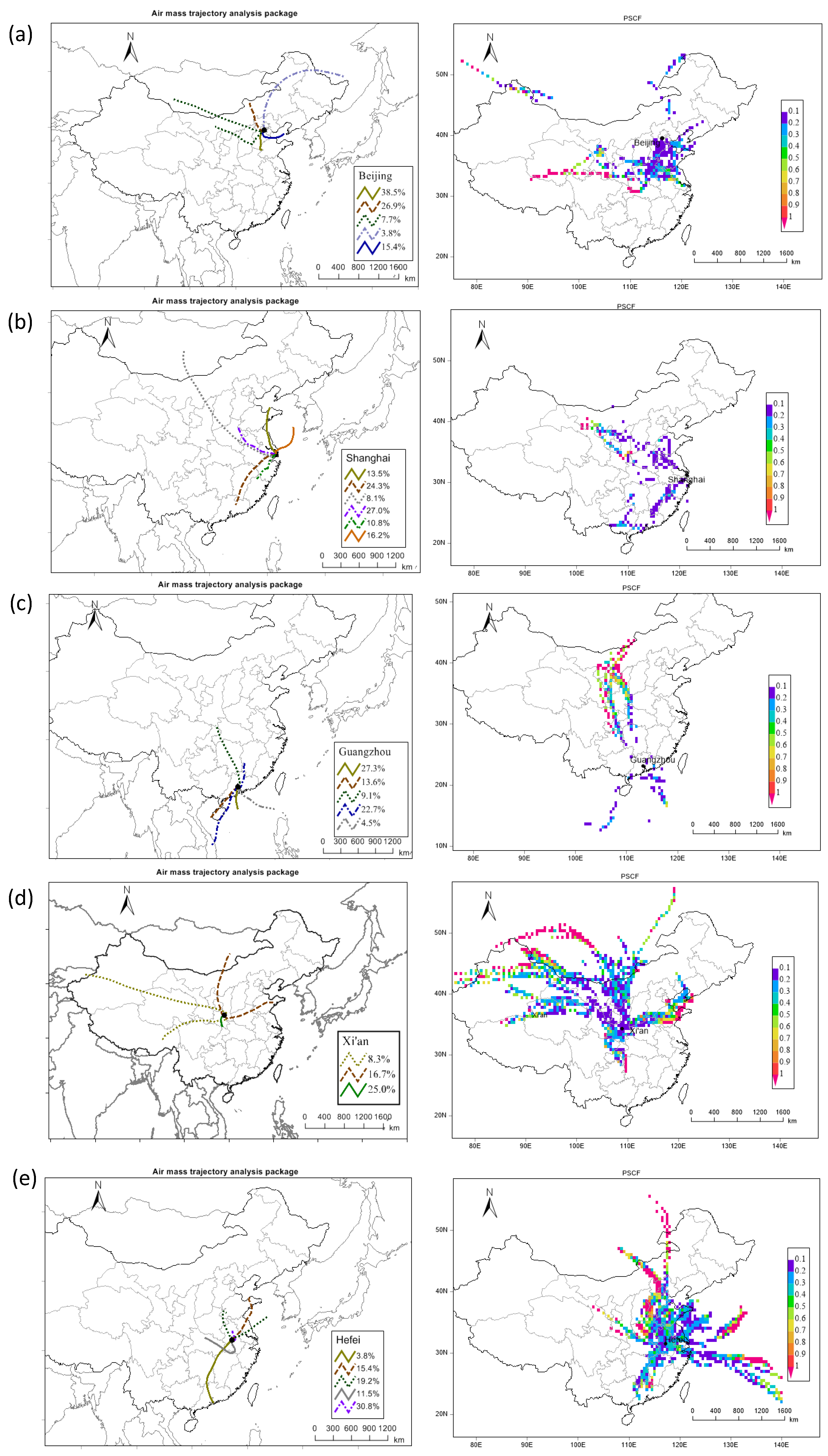
3.5. Transport Pathways of O3 or Its Precursors during O3 Episodes
4. Conclusions
Author Contributions
Funding
Conflicts of Interest
References
- Vingarzan, R. A review of surface ozone background levels and trends. Atmos. Environ. 2004, 38, 3431–3442. [Google Scholar] [CrossRef]
- Thompson, M.L.; Reynolds, J.; Cox, L.H.; Guttorp, P.; Sampson, P.D. A review of statistical methods for the meteorological adjustment of tropospheric ozone. Atmos. Environ. 2001, 35, 617–630. [Google Scholar] [CrossRef]
- Monks, P.S. Gas-phase radical chemistry in the troposphere. Chem. Soc. Rev. 2005, 34, 376–395. [Google Scholar] [CrossRef]
- Shen, Z.; Cao, J.; Zhang, L.; Zhao, Z.; Dong, J.; Wang, L.; Wang, Q.; Li, G.; Liu, S.; Zhang, Q. Characteristics of surface O3 over Qinghai Lake area in Northeast Tibetan Plateau, China. Sci. Total Environ. 2014, 500, 295–301. [Google Scholar] [CrossRef]
- Monks, P.S.; Archibald, A.; Colette, A.; Cooper, O.; Coyle, M.; Derwent, R.; Fowler, D.; Granier, C.; Law, K.S.; Mills, G. Tropospheric ozone and its precursors from the urban to the global scale from air quality to short-lived climate forcer. Atmos. Chem. Phys. 2015, 15, 8889–8973. [Google Scholar] [CrossRef]
- WHO. Review of Evidence on Health Aspects of Air Pollution: REVIHAAP project: Final Technical Report; WHO Regional Office for Europe Copenhagen: København, Danmark, 2013. [Google Scholar]
- Turner, M.C.; Jerrett, M.; Pope, C.A., III; Krewski, D.; Gapstur, S.M.; Diver, W.R.; Beckerman, B.S.; Marshall, J.D.; Su, J.; Crouse, D.L. Long-term ozone exposure and mortality in a large prospective study. Am. J. Respir. Crit. Care Med. 2016, 193, 1134–1142. [Google Scholar] [CrossRef] [PubMed]
- Jerrett, M.; Burnett, R.T.; Pope, C.A., III; Ito, K.; Thurston, G.; Krewski, D.; Shi, Y.; Calle, E.; Thun, M. Long-term ozone exposure and mortality. N. Engl. J. Med. 2009, 360, 1085–1095. [Google Scholar] [CrossRef] [PubMed]
- Fowler, D.; Amann, M.; Anderson, F.; Ashmore, M.; Cox, P.; Depledge, M.; Derwent, D.; Grennfelt, P.; Hewitt, N.; Hov, O. Ground-level ozone in the 21st century: Future trends, impacts and policy implications. In Royal Society Science Policy Report; UEA Digital Repository: Norwich, UK, 2008; Volume 15. [Google Scholar]
- Simon, H.; Reff, A.; Wells, B.; Xing, J.; Frank, N. Ozone trends across the United States over a period of decreasing NOx and VOC emissions. Environ. Sci. Technol. 2014, 49, 186–195. [Google Scholar] [CrossRef] [PubMed]
- Cooper, O.R.; Parrish, D.; Ziemke, J.; Cupeiro, M.; Galbally, I.; Gilge, S.; Horowitz, L.; Jensen, N.; Lamarque, J.-F.; Naik, V. Global distribution and trends of tropospheric ozone: An observation-based review. Elem. Sci. Anthr. 2014, 2, 000029. [Google Scholar] [CrossRef]
- Wang, T.; Xue, L.; Brimblecombe, P.; Lam, Y.F.; Li, L.; Zhang, L. Ozone pollution in China: A review of concentrations, meteorological influences, chemical precursors, and effects. Sci. Total Environ. 2017, 575, 1582–1596. [Google Scholar] [CrossRef]
- Wang, W.-N.; Cheng, T.-H.; Gu, X.-F.; Chen, H.; Guo, H.; Wang, Y.; Bao, F.-W.; Shi, S.-Y.; Xu, B.-R.; Zuo, X. Assessing spatial and temporal patterns of observed ground-level ozone in China. Sci. Rep. 2017, 7, 3651. [Google Scholar] [CrossRef] [PubMed]
- Zhang, H.; Wang, Y.; Hu, J.; Ying, Q.; Hu, X.-M. Relationships between meteorological parameters and criteria air pollutants in three megacities in China. Environ. Res. 2015, 140, 242–254. [Google Scholar] [CrossRef] [PubMed]
- Li, R.; Wang, Z.; Cui, L.; Fu, H.; Zhang, L.; Kong, L.; Chen, W.; Chen, J. Air pollution characteristics in China during 2015–2016: Spatiotemporal variations and key meteorological factors. Sci. Total Environ. 2019, 648, 902–915. [Google Scholar] [CrossRef] [PubMed]
- Gong, X.; Hong, S.; Jaffe, D.A. Ozone in China: Spatial distribution and leading meteorological factors controlling O3 in 16 Chinese cities. Aerosol Air Qual. Res. 2018, 18, 2287–2300. [Google Scholar] [CrossRef]
- Lu, X.; Hong, J.; Zhang, L.; Cooper, O.R.; Schultz, M.G.; Xu, X.; Wang, T.; Gao, M.; Zhao, Y.; Zhang, Y. Severe surface ozone pollution in China: A global perspective. Environ. Sci. Technol. Lett. 2018, 5, 487–494. [Google Scholar] [CrossRef]
- An, Z.; Huang, R.-J.; Zhang, R.; Tie, X.; Li, G.; Cao, J.; Zhou, W.; Shi, Z.; Han, Y.; Gu, Z. Severe haze in Northern China: A synergy of anthropogenic emissions and atmospheric processes. Proc. Natl. Acad. Sci. USA 2019, 116, 8657–8666. [Google Scholar] [CrossRef]
- Chinese State Council. Atmospheric Pollution Prevention and Control Action Plan; Council, C.S., Ed.; Chinese State Council: Beijing, China, 2013. Available online: http://www.gov.cn/zwgk/2013-09/12/content_2486773.htm (accessed on 9 October 2013). (In Chinese)
- Tian, G.; Qiao, Z.; Xu, X. Characteristics of particulate matter (PM10) and its relationship with meteorological factors during 2001–2012 in Beijing. Environ. Pollut. 2014, 192, 266–274. [Google Scholar] [CrossRef]
- Xue, L.; Wang, T.; Gao, J.; Ding, A.; Zhou, X.; Blake, D.; Wang, X.; Saunders, S.; Fan, S.; Zuo, H. Ground-level ozone in four Chinese cities: Precursors, regional transport and heterogeneous processes. Atmos. Chem. Phys. 2014, 14, 13175–13188. [Google Scholar] [CrossRef]
- Li, L.; Qian, J.; Ou, C.-Q.; Zhou, Y.-X.; Guo, C.; Guo, Y. Spatial and temporal analysis of Air Pollution Index and its timescale-dependent relationship with meteorological factors in Guangzhou, China, 2001–2011. Environ. Pollut. 2014, 190, 75–81. [Google Scholar] [CrossRef]
- Shen, Z.; Cao, J.; Arimoto, R.; Han, Z.; Zhang, R.; Han, Y.; Liu, S.; Okuda, T.; Nakao, S.; Tanaka, S. Ionic composition of TSP and PM2.5 during dust storms and air pollution episodes at Xi’an, China. Atmos. Environ. 2009, 43, 2911–2918. [Google Scholar] [CrossRef]
- Han, Y.; Du, P.; Cao, J.; Eric, S.P. Multivariate analysis of heavy metal contamination in urban dusts of Xi’an, Central China. Sci. Total Environ. 2006, 355, 176–186. [Google Scholar]
- Hu, J.; Wang, Y.; Ying, Q.; Zhang, H. Spatial and temporal variability of PM2.5 and PM10 over the North China Plain and the Yangtze River Delta, China. Atmos. Environ. 2014, 95, 598–609. [Google Scholar] [CrossRef]
- Wang, Y.; Zhang, X.; Draxler, R.R. TrajStat: GIS-based software that uses various trajectory statistical analysis methods to identify potential sources from long-term air pollution measurement data. Environ. Model. Softw. 2009, 24, 938–939. [Google Scholar] [CrossRef]
- Wu, Y.; Zhang, S.; Hao, J.; Liu, H.; Wu, X.; Hu, J.; Walsh, M.P.; Wallington, T.J.; Zhang, K.M.; Stevanovic, S. On-road vehicle emissions and their control in China: A review and outlook. Sci. Total Environ. 2017, 574, 332–349. [Google Scholar] [CrossRef] [PubMed]
- NBSC. China Statistical Yearbook 2015; National Bureau of Statistic of China (NBSC): Beijing, China, 2015. (In Chinese) [Google Scholar]
- MEP, C. Ambient Air Quality Standards. GB 3095-2012; China Environmental Science Press: Beijing, China, 2012. [Google Scholar]
- Wang, X.; Shen, Z.; Cao, J.; Zhang, L.; Liu, L.; Li, J.; Liu, S.; Sun, Y. Characteristics of surface ozone at an urban site of Xi’an in Northwest China. J. Environ. Monit. 2012, 14, 116–126. [Google Scholar] [CrossRef]
- Shao, M.; Zhang, Y.; Zeng, L.; Tang, X.; Zhang, J.; Zhong, L.; Wang, B. Ground-level ozone in the Pearl River Delta and the roles of VOC and NOx in its production. J. Environ. Manag. 2009, 90, 512–518. [Google Scholar] [CrossRef]
- Xie, M.; Zhu, K.; Wang, T.; Chen, P.; Han, Y.; Li, S.; Zhuang, B.; Shu, L. Temporal characterization and regional contribution to O3 and NOx at an urban and a suburban site in Nanjing, China. Sci. Total Environ. 2016, 551, 533–545. [Google Scholar] [CrossRef]
- Wang, Y.; Hu, B.; Ji, D.; Liu, Z.; Tang, G.; Xin, J.; Zhang, H.; Song, T.; Wang, L.; Gao, W.; et al. Ozone weekend effects in the Beijing–Tianjin–Hebei metropolitan area, China. Atmos. Chem. Phys. 2014, 14, 2419–2429. [Google Scholar] [CrossRef]
- Tang, W.; Zhao, C.; Geng, F.; Peng, L.; Zhou, G.; Gao, W.; Xu, J.; Tie, X. Study of ozone “weekend effect” in Shanghai. Sci. China Ser. D Earth Sci. 2008, 51, 1354–1360. [Google Scholar] [CrossRef]
- Pont, V.; Fontan, J. Comparison between weekend and weekday ozone concentration in large cities in France. Atmos. Environ. 2001, 35, 1527–1535. [Google Scholar] [CrossRef]
- Abeleira, A.J.; Farmer, D.K. Summer ozone in the northern Front Range metropolitan area: Weekend–weekday effects, temperature dependences, and the impact of drought. Atmos. Chem. Phys. 2017, 17, 6517–6529. [Google Scholar] [CrossRef]
- Tong, L.; Zhang, H.; Yu, J.; He, M.; Xu, N.; Zhang, J.; Qian, F.; Feng, J.; Xiao, H. Characteristics of surface ozone and nitrogen oxides at urban, suburban and rural sites in Ningbo, China. Atmos. Res. 2017, 187, 57–68. [Google Scholar] [CrossRef]
- Wang, T.; Cheung, V.T.; Anson, M.; Li, Y. Ozone and related gaseous pollutants in the boundary layer of eastern China: Overview of the recent measurements at a rural site. Geophys. Res. Lett. 2001, 28, 2373–2376. [Google Scholar] [CrossRef]
- Kalabokas, P.D.; Viras, L.G.; Bartzis, J.G.; Repapis, C.C. Mediterranean rural ozone characteristics around the urban area of Athens. Atmos. Environ. 2000, 34, 5199–5208. [Google Scholar] [CrossRef]
- Kley, D.; Geiss, H.; Mohnen, V.A. Tropospheric ozone at elevated sites and precursor emissions in the United States and Europe. Atmos. Environ. 1994, 28, 149–158. [Google Scholar] [CrossRef]
- Zhao, S.; Yu, Y.; Yin, D.; Qin, D.; He, J.; Dong, L. Spatial patterns and temporal variations of six criteria air pollutants during 2015 to 2017 in the city clusters of Sichuan Basin, China. Sci. Total Environ. 2018, 624, 540–557. [Google Scholar] [CrossRef]
- Wang, Y.; Ying, Q.; Hu, J.; Zhang, H. Spatial and temporal variations of six criteria air pollutants in 31 provincial capital cities in China during 2013–2014. Environ. Int. 2014, 73, 413–422. [Google Scholar] [CrossRef]
- Wang, G.; Zhang, R.; Gomez, M.E.; Yang, L.; Zamora, M.L.; Hu, M.; Lin, Y.; Peng, J.; Guo, S.; Meng, J. Persistent sulfate formation from London Fog to Chinese haze. Proc. Natl. Acad. Sci. USA 2016, 113, 13630–13635. [Google Scholar] [CrossRef]
- Coates, J.; Mar, K.A.; Ojha, N.; Butler, T.M. The influence of temperature on ozone production under varying NO x conditions–A modelling study. Atmos. Chem. Phys. 2016, 16, 11601–11615. [Google Scholar] [CrossRef]
- Tu, J.; Xia, Z.-G.; Wang, H.; Li, W. Temporal variations in surface ozone and its precursors and meteorological effects at an urban site in China. Atmos. Res. 2007, 85, 310–337. [Google Scholar] [CrossRef]
- Lal, S.; Naja, M.; Subbaraya, B. Seasonal variations in surface ozone and its precursors over an urban site in India. Atmos. Environ. 2000, 34, 2713–2724. [Google Scholar] [CrossRef]
- Roberts–Semple, D.; Song, F.; Gao, Y. Seasonal characteristics of ambient nitrogen oxides and ground–level ozone in metropolitan northeastern New Jersey. Atmos. Pollut. Res. 2012, 3, 247–257. [Google Scholar] [CrossRef]
- Gaudel, A.; Cooper, O.; Ancellet, G.; Barret, B.; Boynard, A.; Burrows, J.; Clerbaux, C.; Coheur, P.-F.; Cuesta, J.; Cuevas Agulló, E. Tropospheric Ozone Assessment Report: Present-day Distribution and Trends of Tropospheric Ozone Relevant to Climate and Global Atmospheric Chemistry Model Evaluation; University of California Press: Berkeley, CA, USA, 2018. [Google Scholar]
- Zhao, S.; Yu, Y.; Yin, D.; He, J.; Liu, N.; Qu, J.; Xiao, J. Annual and diurnal variations of gaseous and particulate pollutants in 31 provincial capital cities based on in situ air quality monitoring data from China National Environmental Monitoring Center. Environ. Int. 2016, 86, 92–106. [Google Scholar] [CrossRef] [PubMed]
- Guenther, A.; Hewitt, C.N.; Erickson, D.; Fall, R.; Geron, C.; Graedel, T.; Harley, P.; Klinger, L.; Lerdau, M.; McKay, W. A global model of natural volatile organic compound emissions. J. Geophys. Res. Atmos. 1995, 100, 8873–8892. [Google Scholar] [CrossRef]
- National Research Council. Energy Futures and Urban Air Pollution: Challenges for China and the United States; National Academies Press: Cambridge, MA, USA, 2008. [Google Scholar]


| City | O3 (µg·m−3) | Exceedance (days) 2 | |||
|---|---|---|---|---|---|
| Mean | S.D. 1 | Min | Max | ||
| Beijing | 98.4 | 64.0 | 1.0 | 311.9 | 116 |
| Shanghai | 100.1 | 43.0 | 14.4 | 272.8 | 52 |
| Guangzhou | 91.5 | 49.7 | 2.0 | 285.6 | 64 |
| Xi’an | 61.6 | 44.2 | 3.0 | 205.4 | 20 |
| Hefei | 43.7 | 44.0 | 5.0 | 235.6 | 28 |
| NO2 | CO | SO2 | PM2.5 | PM10 | Temp | RH | WS | ||
|---|---|---|---|---|---|---|---|---|---|
| Beijing, MDA8 O3 | spring | 0.12 | 0.06 | 0.08 | 0.32 ** | 0.29 ** | 0.73 ** | 0.38 ** | 0.07 |
| summer | 0.52 ** | 0.41 ** | 0.36 ** | 0.61 ** | 0.65 ** | 0.35 ** | 0.05 | 0.11 | |
| autumn | −0.58 ** | −0.44 ** | −0.31 ** | −0.22 ** | −0.19 ** | 0.71 ** | −0.21 ** | 0.15 | |
| winter | −0.77 ** | −0.68 ** | −0.50 ** | −0.61 ** | −0.47 ** | −0.12 | −0.40 ** | 0.14 | |
| Shanghai, MDA8 O3 | spring | 0.11 | −0.18 * | 0.05 | 0.25 ** | 0.36 ** | 0.51 ** | −0.21 ** | −0.01 |
| summer | 0.21 ** | 0.19 * | 0.44 ** | 0.58 ** | 0.48 ** | 0.15 | −0.17 * | −0.09 | |
| autumn | −0.21 ** | 0.03 | 0.05 | 0.10 | 0.13 | 0.61 ** | −0.15 | −0.07 | |
| winter | −0.44 ** | −0.23 ** | −0.29 ** | −0.17 * | −0.18 * | 0.10 | 0.12 | 0.21 ** | |
| Guangzhou, MDA8 O3 | spring | 0.10 | 0.01 | 0.49 ** | 0.32 ** | 0.45 ** | 0.34 ** | −0.37 ** | 0.06 |
| summer | −0.06 | 0.07 | 0.37 ** | 0.48 ** | 0.63 ** | 0.52 ** | −0.52 ** | −0.39 ** | |
| autumn | 0.26 ** | −0.13 | 0.40 ** | 0.68 ** | 0.61 ** | 0.00 | −0.14 | 0.24 ** | |
| winter | 0.06 | 0.00 | 0.45 ** | 0.48 ** | 0.43 ** | 0.05 | −0.30 ** | −0.37 ** | |
| Xi’an, MDA8 O3 | spring | −0.27 ** | −0.26** | −0.12 | −0.06 | −0.27 ** | 0.56 ** | −0.25** | 0.13 |
| summer | 0.12 | −0.15* | 0.16 * | 0.20 ** | 0.15 * | 0.54 ** | −0.30 ** | 0.32 ** | |
| autumn | −0.23 ** | −0.36** | −0.26 ** | −0.07 | −0.17 * | 0.60 ** | −0.14 | 0.27 ** | |
| winter | −0.17 * | 0.05 | −0.23 ** | −0.01 | 0.06 | 0.16 * | −0.10 | 0.15 | |
| Hefei, MDA8 O3 | spring | 0.12 | 0.14 | 0.73 ** | −0.26 ** | −0.01 | −0.19 ** | −0.02 | −0.00 |
| summer | −0.25 ** | 0.03 | 0.06 | 0.11 | 0.34 ** | −0.18 * | −0.07 | 0.01 | |
| autumn | 0.97 ** | 0.09 | 0.42 ** | 0.04 | −0.15 | −0.13 | −0.09 | 001 | |
| winter | 0.07 | 0.02 | −0.19 * | −0.12 | 0.09 | 0.02 | 0.23 ** | 0.06 | |
| City | Short-Distance Transport | Long-Distance Transport | ||
|---|---|---|---|---|
| Air Mass Source | Proportion | Transport Pathway | Proportion | |
| Beijing | Shijiazhuang | 38.5% | Mongolia-Inner Mongolia-Shanxi-Hebei | 7.7% |
| Inner Mongolia | 26.9% | Russia-Heilongjiang-Inner Mongolia-Hebei | 3.8% | |
| Tianjin | 15.4% | |||
| Shanghai | Anhui | 27.0% | Guangdong-Jiangxi-Anhui | 24.3% |
| Yellow Sea | 16.2% | |||
| Jiangsu | 13.5% | Mongolia-Inner Mongolia-Shaanxi-Shanxi-Henan-Anhui | 8.1% | |
| Zhejiang | 10.8% | |||
| Guangzhou | South China Sea | 27.3% | South Jiangxi -North Guangdong; South China Sea-Hainan Island | 22.7% |
| Chongqing-Hubei-Hunan | 9.1% | |||
| Hainan | 13.6% | Dongsha Islands | 4.5% | |
| Xi’an | Qinling Mountain | 25.0% | Mongolia-Inner Mongolia-Ningxia; Shandong-Henan | 16.7% |
| Xinjiang-Qinghai-South Gansu; East Tibet-North Sichuang | 8.3% | |||
| Hefei | Huainan | 30.8% | Shandong Peninsula-Jiangsu | 15.4% |
| Hubei-Jiangxi-South Anhui | 11.5% | |||
| East Henan-Jiangsu | 19.2% | Guangdong-Hunan-Hubei | 3.8% | |
© 2020 by the authors. Licensee MDPI, Basel, Switzerland. This article is an open access article distributed under the terms and conditions of the Creative Commons Attribution (CC BY) license (http://creativecommons.org/licenses/by/4.0/).
Share and Cite
Wang, X.; Shen, Z.; Tang, Z.; Li, G.; Lei, Y.; Zhang, Q.; Zeng, Y.; Xu, H.; Cao, J.; Zhang, R. Characteristics of Surface Ozone in Five Provincial Capital Cities of China during 2014–2015. Atmosphere 2020, 11, 107. https://doi.org/10.3390/atmos11010107
Wang X, Shen Z, Tang Z, Li G, Lei Y, Zhang Q, Zeng Y, Xu H, Cao J, Zhang R. Characteristics of Surface Ozone in Five Provincial Capital Cities of China during 2014–2015. Atmosphere. 2020; 11(1):107. https://doi.org/10.3390/atmos11010107
Chicago/Turabian StyleWang, Xin, Zhenxing Shen, Zhuoyue Tang, Guohui Li, Yali Lei, Qian Zhang, Yaling Zeng, Hongmei Xu, Junji Cao, and Renjian Zhang. 2020. "Characteristics of Surface Ozone in Five Provincial Capital Cities of China during 2014–2015" Atmosphere 11, no. 1: 107. https://doi.org/10.3390/atmos11010107
APA StyleWang, X., Shen, Z., Tang, Z., Li, G., Lei, Y., Zhang, Q., Zeng, Y., Xu, H., Cao, J., & Zhang, R. (2020). Characteristics of Surface Ozone in Five Provincial Capital Cities of China during 2014–2015. Atmosphere, 11(1), 107. https://doi.org/10.3390/atmos11010107