Abstract
The study presents a newly generated hindcast database of metocean conditions for the region of the North Sea by parametrising the newly introduced ST6 physics in a nearshore wave model. Exploring and assessing the intricacies in wave generation are vital to produce a reliable hindcast. The new parametrisations perform better, though they have a higher number of tuneable options. Parametrisation of the white capping coefficient within the ST6 package improved performance with significant differences ≈±20–30 cm. The configuration which was selected to build the database shows a good correlation ≈ for , has an overall minimal bias with the majority of locations being slightly over-estimated ±0.5–1 cm. The calibrated model was subsequently used to produce a database for 38 years, analysing and discussing the metocean condition. In terms of wave energy resource, the North Sea has not received attention due to its perceived “lower” resource. However, from analysing the long-term climatic data, it is evident that the level of metocean conditions, and subsequently wave power, can prove beneficial for development. The 95th percentile indicates that the majority of the time should be expected at 3.4–5 m, and the wave energy period at 5–7 s. Wave power resource exceeds 15 kW/m at locations very close to the coast, and it is uniformly reduced as we move to the Southern parts, near the English Channel, with values there being ≈5 kW/m, with most energetic seas originating from the North East. Results by the analysis show that in the North Sea, conditions are moderate to high, and the wave energy resource, which has been previously overlooked, is high and easily accessible due to the low distance from coasts. The study developed a regional high-fidelity model, analysed metocean parameters and properly assessed the energy content. Although, the database and its results can have multiple usages and benefit other sectors that want to operate in the harsh waters of the North Sea.
1. Introduction
The marine environment is host to a variety of human activities, and its investigation can contribute in design parameters for a plethora of applications spanning from coastal infrastructure, to energy, ship design, tourism and more. Therefore, it is safe to say that amongst the most vital components for any application in the offshore environment is the knowledge of metocean conditions that can change over time. This is becoming more prevalent due to climate change effects, which are amongst the main drivers for wave generation conditions, leading to direct effects of coastal flooding, storm surges and coastal erosion [1,2,3].
Reguero et al. [4] examined the global wave conditions, making the observation that wave power has increased potentially due to anthropogenic emissions. Metocean parameters such as significant wave height () and period(s) display differences since their 1948 levels, and will tend to alter in the years to come. However, this is not universally distributed along the globe; further exploration regional analysis must be undertaken to determine the metocean characteristics accurately. Long-term high fidelity spatio-temporal data are very important for analysis on wave conditions [5], wave power resource [6], extreme value analysis [1,7], and climate characteristics [3,8], etc.
To obtain necessary information, for climate analysis on any type of renewable resource, a minimum duration of 10 years is required [9,10,11,12,13]. Furthermore, to have a good understanding of climate conditions and their persistence, additional considerations on Climatological Standard Normals (CSN) are required. CSN suggest a minimum period that allows long-term extrapolation and proper estimation of averages for climatological parameters, computed for consecutive periods of ≥30 years [14]. Without long-term data, any estimation on coastal infrastructure, or in the case of ocean energies development/estimation of energy production, will be highly flawed, since it will not account resource changes and variability. Hence, it is important to consider the high impact value of resource assessments in any offshore activity.
To date, metocean data have been obtained by three main ways. Firstly, by in-situ measurement devices, such as buoys, acoustic Doppler current profiler (ADCP), gauges and similar deployable equipment. Secondly, via use of satellite and/or altimeter data through the various missions that are in orbit. The third way is via the use of numerical wave models, either phase resolving or phase averaged. Each of these methods has its strengths and weaknesses.
Buoys are most commonly used for in-situ measurements, and can provide a wide array of parameters such as surface elevation, lateral motion, , wave direction (, ), and spectral information. Buoys have relatively good temporal resolution with sampling intervals in the range of 10–30 min, and can be deployed over a long-period of time. However, they do not come without limitations; firstly, measurements are influenced by deployment depth. Wave heights transform as they propagate from deeper to nearshore water due to various physical processes such as depth breaking. This means that their measurements are applicable only at that location and cannot be arbitrary extended over several other “nearby" locations, which may be characterised by different depths and nearby coastal masses. Buoys are also limited by the length of their moorings, affecting their maxima of vertical displacements (in case of extreme events), often slipping around incoming crests and giving erroneous measurements [15]. Finally, their recordings are often not “full”, i.e., hours, days, weeks, months are absent, and their deployments are not continuous but subject to recurring maintenance and re-calibration.
The second source of information, increasingly promising, is satellite altimeter data. After 1991, satellite data started to become available, first datasets from satellites did not had enough temporal recordings and could not be considered for resource assessments [15]. Satellites depend on orbital trajectories, i.e., the interval of which they pass over the same location, some of the “older” satellites recordings can have gaps 10–30 days apart (pending on mission), lately, satellites orbits and samplings have increased in time and can offer information at higher resolution (i.e., every 12 h). This does not mean that they are available immediately, as in the case of buoys.
In fact, most satellite altimeter data have to be corrected and filtered, before any meaningful data are retrieved; this can take up to several months. There is the possibility of shorter releases, so-called real-time products, that are from ongoing missions and are made available within a few hours, but only for specific processes, such as wave forecasting. Another limitation is the fact that satellite altimeter data have “blind” spots when it comes to the nearshore. When trying to measure close to the coastlines ≈20 km they cannot properly distinguish land from water masses [16]. This creates some issues with regards to their performance. Cavaleri et al. [17] compared four different altimeter mission data, and came to the interesting conclusion that in the nearshore, though measurements were obtained, they did not match in magnitude, and depending on data frequency resolution displayed, “noise” measurements at ≤20 km from the coast. Smaller differences were given by surface wind recordings, but the complexity of waves increased the differences , almost by .
The third method to obtain long-term uniform datasets uses Numerical Wave Models (NWM). These tools are under continuous development, and improved upon as more insight into the complex ocean processes is gained. Since the first numerical model attempt [18], NWM provide valuable information for climate change, shipping, energy, weather forecasts, and metocean operations. NWM are able to deliver high fidelity spatio-temporal information, with suitable long-term characteristic for resource assessments. They can have varied resolution, multi-nested domains, and focus at different regions. However, this does not mean that NWM are without limitations. As in any modelling effort, it is paramount that the user/modeller has knowledge of the processes involved, and is able to select the different physical processes, pending on desired application and scale. Currently, there are several models that are able to resolve different physical processes. However, one thing that it is important to note, most processes in NWM are based on (semi-)empirical coefficients and are often very sensitive to local environments. It is of importance for the model to be configured and set-up according to the application. In addition, reliable results have to be obtained by careful validation, after model calibration [19].
Gap in Knowledge
The Netherlands are located in the North Sea and have long been exposed to harsh weather events and danger of floods. The Dutch coastlines often experience severe storms, and due to the position of some cities below the water level, coastal protection has been developed to protect the re-claimed areas. There are several measurement stations dispersed regionally, including a very detailed and well maintained buoy network [20]. The Dutch government has increased its interest in developing offshore renewables and aquaculture in the Dutch Exclusive Economic Area.
The Netherlands do not have a comprehensive resource assessment of wave conditions suitable to describe the wave resource in the nearshore. The majority of information is based on oceanic models and larger area studies, which by default encompass the North Sea in general, but at a very coarse resolution. The wave characterisation at such large scales have been done by several authors with resulted datasets providing important information on the state of Climate Change over the region [3], return values for extreme events [7,21], and climate characterisation [22]. The studies used models that are efficient at larger domains, but have inherit limitation in terms of resolving higher resolution domains and nearshore complexities [19].
The aim of the study is two-fold, first, to assess the effects on new wind scheme parametrisations in a nearshore wave model, and secondly, to fill the gap of knowledge for the metocean conditions in the North Sea. The North Sea Wave Database (NSWD) provides high resolution information, has a long-term duration from 1980 to 2017 (end of 2017, 38 years), and a high temporal resolution of various spectral parameters. Configuration of the nearshore model, specifically tuned for the region is discussed, is presented with a thorough calibration and comparison with in-situ measurements.
Parametrisations assess the performance of a new set of equations, which affect wind generation and whitecapping coefficients. The configuration discussed is applicable to be used with confidence for metocean studies in the region, as the tuning is focused without use of data assimilation or correction parametrisations, and uses open-source datasets. The best fit model is used to develop a 38 years dataset, the North Sea Wave Database (NSWD), with hourly output for various quantities.
Finally, a resource analysis is conducted based on the NSWD, estimating and discussion the spatial distributions and levels of expected variation for various parameters. It also includes an analysis of wave power and accessibility useful for future maintenance and operations activities in the region(s). These information are vital for wave climate analysis, extreme value analysis, the emerging wave power industry, offshore wind and any offshore activity. The areas of highest potential identified can be used for further, higher spatial analysis, and the metocean conditions are valuable to properly assess the energy production capabilities of wave energy converters (WECs), finding the most suitable location and/or WEC. In addition, a resource assessment of such scale is also useful for designing parameters of offshore wind farms, coastal defences and the selection of most suitable vessels (per region) to obtain increased access to assets.
2. Materials and Methods
For generation of the database a third generation spectral phased averaged model, Simulating WAves Nearshore (SWAN) was used. The model has been developed and is maintained by TU Delft [23], the version used is 41.20. However, prior to developing a reliable dataset several considerations must be addressed. Firstly, the construction of useful boundary and feed-in information. For the development of such a long-term dataset we have to ensure that proper methods are used and most importantly a suitable wave model is utilised [19]. The SWAN model is suitable to provide reliable information at the nearshore, as it contains the possibility of modelling complex non-linear interactions that exist near the coastlines. This is highly important, as most first generation wave energy converters (WECs) will be placed near the shoreline, at depths were bathymetry has influence over the metocean conditions.
The methodology for development of an analysis requires thorough calibration and validation of the dataset. Calibration of the model is conducted for the year 2015, after the calibration an “optimal” model is selected and used to generate the 38 year (1980–2017) hindcast. Buoy data are used for calibration evaluation and subsequent validation of the hindcast [20]. In the following sub-sections model inputs and considerations on physical configuration for the calibration, as well as the performance of the solution are presented.
2.1. Modelling Inputs
The model has been set-up with spherical coordinates and a resolution of , corresponding to ≈2.5 km longitude () and ≈2 km latitude (), also accounting for the Earth’s curvature. Coastline data have been obtained by Amante et al. [24] and the latest Global Self-consistent, Hierarchical, High-resolution Geography Database (GSHHG) [25]. Based on this information a bathymetry domain was constructed as input for the model, see Figure 1. The Dutch coastlines are located at a continental shelf, neighbouring Denmark and the United Kingdom. As seen in Figure 1, the depth is varying “smoothly” without the existence of very sharp depth gradients, for the domain of this database depth does not exceed 100 m.
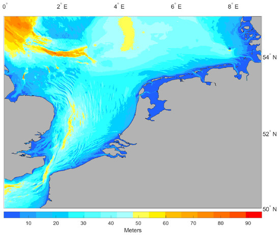
Figure 1.
Developed domain for the study, depth in meters.
As driver of wave generation the ERA-Interim wind dataset, by the European Centre for Medium-Range Weather Forecasts (ECMWF) was utilised [26]. There is a high-correlation between wind resource as a driver, wind-wave generation/propagation and model performance [27]. However, depending on the area, model, and tuning the higher temporal resolution wind fields are not always optimal, for the wider Atlantic [28] and the North Sea [29] both the ERA-Interim and a higher temporal wind field has been explored. The results indicated that “peaks” of high wave were captured better, but the overall performance was significantly lower with greater scattering and a over-bias in higher wave frequencies. Similar, behaviour between different datasets has been also reported in other studies, with ERA-Interim exhibiting good performance with reduced scattering [27]. While, other datasets can have higher temporal resolution, this public domain re-analysis dataset is based on Regional Climate Models closely relatable for the region, and the wind speeds exhibit better performance with measured data for the European continent.
Considering that NSWD is developed for various usage spanning from wave energy to climate analysis, main focus is to reduce the scattering and maintain close agreement with higher wave values therefore minimising over-predicting, as this can lead to over-estimating return values [30], and to higher capital expenditure estimates for infrastructure.
Spectral boundary conditions were re-constructed by the WAve Model (WAM) from ECMWF and applied at domain open boundaries. Most important boundary region is the open upper North side where swell waves from the Atlantic and Norwegian Sea propagate inwards. The model was set-up with a “warm-up” configuration to minimise initial ramp-up periods.
2.2. Calibration Parametrisation
SWAN is a third generation spectral phased-averaged wave model, that accounts multiple physical processes suitable for deep and shallow waters, although arguably it is more efficient for nearshore and Shelf Seas. The wave spectrum is described in time (t) by the action density equation (E), dependent upon angular frequency (), direction (), frequency (f), energy propagation (c) over latitude () and longitude (). Sink source terms are used to estimate the wave parameters (see Equation (1)), given a specific set of inputs and physical coefficients, with wind input (), triads (), quadruplet () interactions, whitecapping (), bottom friction () and () depth breaking.
In wave models, generation, propagation and spectrum evolution is dependent on various parameters. Most important source terms are mechanisms of wind , and dissipation , as they are responsible for wave generation and dissipation. Waves are created by wind surface pressure on the ocean, in wave models this term is modelled by considering a wind drag coefficient () that contributes to the growth. Wind wave generation is a summation of energy density from the (over Spherical coordinates).Wind drag coefficients can differ and may enhance or reduce the wave generation capabilities in the model. With regards to dissipation mechanisms, the most obscure and least understood is the white-capping that is predominately based on a wave steepness coefficient (), depending on a term adjustable and quite different for each methodology. It is known that wave models tend to under-estimate at lower frequencies, with accuracy affected by wind components used.
Recently, SWAN 41.20 introduced an adjusted formulation for wind and whitecapping, similar but not the same to Wavewatch3 (WW3) ST6 [31,32]. The wind drag parametrisation requires fine tuning in the whitecapping coefficient. Interestingly with this new addition the solutions both for the wind drag formulation, stress re-computation, allows for bias wind corrections. In addition, the new formulation can also be configured to include swell dissipation mechanisms. For the models developed an exponential growth coefficient is assigned, and all models have a “hot” start configuration that ensures a fully developed wave field. The sink term of wind input that gives wave generation is given by Equation (2)
where A is the linear growth, and is the exponential growth, both A and depend on wind parametrisations. This in turn affects the momentum flux that is the driver between atmosphere and the ocean surface for wave generation, as the model translates wind at 10 m () to a surface wind, see Equation (3) with an estimation wind drag coefficient () that depends on .
Wind drag estimations have limitations especially for higher wind speeds, where they are known to under-estimate and even limit wave growth, therefore, for every different configuration, the should be adjusted. Kamranzad et al. [33] indicated that even though wind drag parametrisations in models are good at generating waves, they are limited in their performance especially at higher wind values, where wave growth reduces, see Figure 2. To alleviate this limitation, a modified formulation was used and since 41.20, a similar approach to that of Rogers et al. [34] can be activated.

Figure 2.
Performance of wind drag coefficient (with author’s permission [33]).
The performance of the wave model depends highly on the parametrisation of the wind sceme, therefore, four different wind schemes have been used and parameterized to obtain the optimal solution. The explanatory naming sequence of the models is based first on the wind configuration used, more specifically for the ST6 (wind 4) package the naming is ST Wind4 x Opt x Scale x, resulting in a numeric name for the model i.e., STE121 meaning a model that utilises the WAM4 wind configuration, with option 2 (for local & cumulative dissipation) and Scale 1, see Figure 3. For Wind 1 the configuration uses Komen et al. [35] set-up, where the wind drag coefficient () is dependent on the friction velocity of wind speed () with adjustments and , see Equation (4). For Wind 2 the adjustments are based on Janssen [36], where critical height is iteratively estimated according to its non-dimensional value from , see Equation (5). For Wind 3 option drag is based on the alternative description of van der Westhuysen et al. [37], that uses a re-formulation of whitecapping to weakly and strongly forced waves.
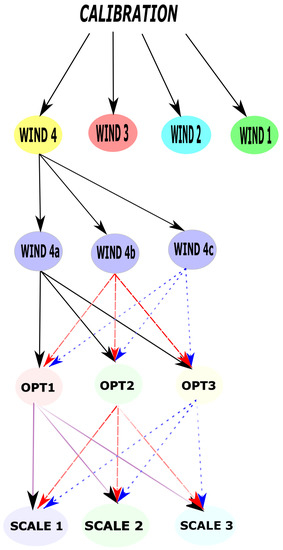
Figure 3.
Configuration for the calibration phase.
Wind 4 represents the newly added ST6 package, and evaluates a different parametrisation in wind drag (see Equation (6)), wind stress and whitecaps [38]. This newly adopted package is similar to WWIII but they are implemented differently. The package includes influence of swell dissipation in the estimations. Wind 4a the is adjusted according to Hwang et al. [39], in wind 4b according to Fan et al. [40] and Wind 4c based on Janssen [36]. Within all different wind configurations, the stress calculation is iteratively vectorally estimated. This means that higher wind speeds are better represented and higher magnitude waves are better resolved.
For whitecapping, Wind 1 and 4 use [35] (WAM3 cycle), but a noticeable difference of the ST6 package, from WWIII and the other SWAN options for whitecaps is the use of a swell steepness dependent dissipation coefficient, is set at 1.2 according to Ardhuin et al. [41]. Wind 2 uses the WAM4 cycle formulation [42]. Bottom friction has been adjusted according to Zijlema et al. [43] 0.038 , nearshore breaking, triad interactions, and diffraction are all enabled based on their respective suggested values in SWAN. Quadruplets interactions for deeper water are resolved with a fully explicit computation per sweep, which makes the computation a bit more “expensive”, but retains good agreement.
In the ST6, dissipation is described by local and cumulative terms, that can be accordingly scaled; based on previous works on derivation of these terms, the following “pairs” are utilised for dissipation (whitecapping effects) [34,38]. Option 1 has local dissipation (lds): 5.7 cumulative dissipation (cds): 8, option 2 lds: 4.7, cds: 6.6, and option 3 lds: 2.8, cds: 3.5. The scaling option parametrisation aims to correct the mean square slope, in this new term, the suggestion is that the scale is over 28. Therefore, seeking to ensure a potential noticeable improvement, we opted for three different tuning parameters, scale 1:28, scale 2:32 and scale 3:35. Whilst more scaling can be attempted, it is expected that the difference from 28 to 35 will be adequate to display any impacts on the hindcast. Tuning this option has to do with how much energy (more or less) is allowed to migrate in higher frequencies. The higher the number, the lower the amounts that are allowed there, therefore, this can be beneficial to not under-estimate lower frequencies. All calibration models were tuned using the binned distribution of 36 directions and frequencies, with the latter using a = 0.1. The calibrations were conducted with an Intel Xeon with 36 GB of RAM.
To assess model results, several indices are used, Pearson’s correlation coefficient (R) indicates how well the hindcast performed (see Equation (7)), the root-mean-square-error () underlines the differences between hindcast and buoy measurements (see Equation (8)), the Scatter Index () give an indication on the relationship between observed and modelled data (see Equation (9)). The goal of a good hindcast is to obtain high correlation values of significant wave height () 85–90%, with small showing a close “positioning” with the mean values, a low 25–30% (or high inverse 85–90%) indicating that the trends are well followed. From experience we are aware that wave models have a tendency to under-estimate, therefore, we also compare the maximum values of significant wave height (), to ensure that not only the mean bias is low (see Equation (10)), but the bias of maxima of events is also reduced by the model. This is considered helpful as it will translate to improvements in statistically estimating extreme return wave periods, and making the final model more versatile.
where is the simulated wave parameter, recorded and N measurements. Finally, the Model Performance Index (MPI) diagnosis performance, indicating the degree to which the model reproduces observed changes of the waves ().
The primary focus of the calibration is to ensure a good re-production of past wave events in order to develop a wave power database. To examine the model, wave data from buoy measurements were gathered [44], filtered by removing non-operational days, see Table 1 and Figure 4 for their locations in the domain.

Table 1.
Buoy information and compared data length.

Figure 4.
Bathymetry domain depth in meters and locations as numbered in Table 1.
3. Results and Analysis
3.1. Calibration
In total, 30 calibration models were assessed and their performance was determined by taking into account the aforementioned indices and runtime. From experience, we are aware that using the ERA-Interim dataset will reduce the maxima performance if no calibration of the whitecapping coefficient is made [29,45]; so as a final qualitative metric, we also examined the ability of modelled data to be close to maximum wave height value. Ideally, the bias will be near zero, and the maximum values will be closely followed, as they are important for extreme value analysis, moorings and structural estimations. If we were only interested in obtaining higher maxima values, we would have opted for using Climate Forecast System Reanalysis (CFSR) data which have shown a better maximum peak performance with means over-estimations and larger scattering in the North Sea [29].
In Figure 5, the histograms of significant wave height () for all calibration models are given, each model was compared with the ten buoys, see Table 1, to assess the performance. All locations were compared with in-situ measurements and the most suitable model was selected. For most locations showed a high R from 93 to 97%, the mean bias is clustered at small under-estimations for with total number of 300 compared locations by all calibrated models having a very small difference from −0.5 to 0.1 m, the is also limited with most compared data from 0.3 to 0.6 m. Finally, scattering of the results is within 18–25%, showing a strong agreement, see Table 2.
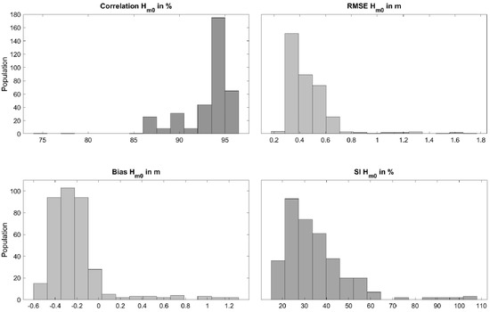
Figure 5.
Histograms of indices for all compared locations by all calibration models.
Table 2.
Aggregate calibration performance for all locations.
Performance of the mean zero crossing period () shows good agreement but with lowered correlations when compared with , see Figure 5. For the coefficient shows that most skilled models are within the range of 80–90% (see Figure 6), the RMSE is quite low from 0.5–1.5 s. This leads to a very small bias with most results showing small under-estimations in line with the performance for mean bias. Finally, the calibration mean biases are located in the density of 20–27%, see Table 2.
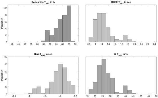
Figure 6.
Histograms of indices for all compared locations by all calibration models.
The histograms show that all configurations are able to hindcast wave quantities in close agreement, however, only one model configuration can be selected for the NSWD hindcast. Most models offer good correlations and almost all have small under-estimations. Figure 7 shows R and inverse with regards to for all the models at platform F3 ( East, North). Following the trend of histograms, most models have a good R, the highest one is given by the with 96% and SI 20% (inverse 80%). However, when also accounting for the other indices , , have better performance with lower SI (19%), a significant low bias −0.04 m, in contrast bias is −0.18 m, the is also smaller with 0.35 m for the STH “family” and 0.37 m for . For all ST6 “families” that share the same wind drag and scale coefficients, they have almost identical performance, indicatively for the F3 location there are differences based on rate of dissipation, these alteration have predominately effects on bias and maxima shown in Table 3 and Figure 7 for F3.

Figure 7.
Comparison of calibrating models, with dotted lines are the mean of each quantity for all models.
Table 3.
platform F3 calibration results .
With such small differences in use of ST6, the maximum value of is also used as a metric of merit. For example, at F3 the recorded maximum is 7.98 m, therefore it was also considered that the calibrated model should also be able to overcome the often under-performance in maxima. The calibration models with the first wind drag and third scaling coefficient achieved the highest maxima, therefore these seem to be the most “accurate” configuration, see Figure 8 and Figure 9. Since the indices have little to no difference, the run time to complete the hindcast was also assessed. The hindcast configuration has to be the one with highest correlation, closest maximum, lowest biases, , but at the same time must also be computational economical. As it can be seen from Figure 9, the generation trend is closely followed and the maxima of recorded waves are also well captured. Assessment of all buoy location was conducted for all configurations and out of the 30 calibration models, was found to be 27 times better, followed by three times for (comparison with 300 resulted points ten locations per calibration).

Figure 8.
of the “good model” based on ST6 parametrisation.
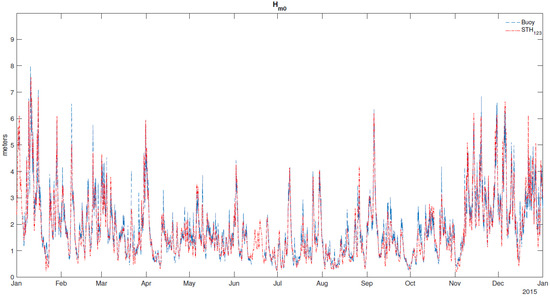
Figure 9.
Comparison of in-situ data with “good” configuration model.
When compared with the exhibits 10 cm difference in at nearshore regions and 15 cm at deeper waters (see Figure 10), indicating that there would be significant under-estimation of the propagating wave fields and subsequently of potential energy flux. The spatial differences between Hwang calibration models is very small in the effect of ≈, when also compared with the other wind configuration then majority of differences is found at deep and nearshore areas, when the “optimal” configuration is assessed with the similar option and scale but different wind drag , the highest difference is ≈12 cm at deep waters, and 1–2 cm along the coastlines. When compared with , then there is a higher difference ≈18 cm and 3–4 cm for deeper and nearshore regions respectively.

Figure 10.
differences of means in meters for versus the .
3.2. Validation
Valuable in information which can properly represent metocean conditions and allow for estimation of climate statistics, wave energy, have to include at least 10 years of un-interrupted homogenous data, with at least 3 h of temporal resolution, and favourably ≥30 years [11,14]. This is extremely important as renewable resources are climate dependent and have to be properly resolved. When estimating the resource content, and potential energy output or wave characteristics a long-term suitable dataset can be confidently used for the next 20 years.
Through the calibration an “optimal” model configuration was selected, and is applied to hindcast data for the needs of metocean and wave energy assessment in the North Sea for 38 years, from 1980–2017. Onwards this specific hindcast database will be denoted as North Sea Wave Database (NSWD). The NSWD is homogenous and all available years are compared with in-situ buoy measurements to assess confidence. In-situ measurements are dispersed and located at various depths, focus is given especially at nearshore and shallow water locations, which are both of imminent interest for wave energy deployments and where larger oceanic models have limitation. All available buoy locations were filtered, analysed and compared with NSWD, validation results are given in Table 4 and Table 5.
Table 4.
Validation of for all available locations.
Table 5.
Validation of for all available locations.
There is never gonna be a “perfect” model, however by utilising a calibrated/validated model, we can identify the areas of interest and/or limitations. Subsequently, additional analysis can be developed, with higher focus to specific regions via use of multi-domain nesting. The NSWD hindcast allows such future cases to be developed at later stages, as the primary domain contains information relevant for re-constructing internal boundary condition.
The majority of locations indicate a high agreement for with R within ≈90–94%. For Southern parts of Dutch coastlines (Brouwershavensegat, Europlatform 3, Schouwenbank, Eurogeul DWE), R shows a high agreement following the generation trend. Most of the years exhibit a good MPI with values consistently over ≥98%. Regarding the bias performance, expect from Schouwenbank, all modelled data show an over-estimation by ≈10–20 cm. In Schouwenbank, there is an under-estimation of the same magnitude. It has to be noted that while usually the bias is used as a good order of merit, we have decided to also look into the maxima values differences. Although, this can somewhat inferred by the Scatter Index (i.e., a low scatter index, may indicate good “maxima” capture). Unlike, the trend of bias slight over-estimation, most maxima values are only slightly under-estimated, usually with a difference of ≈30–80 cm. However, there is an instance where the modelled data under-estimated significantly with 1.28 m at Brouwershavensegat in 2012. For the assessment of the trend of generation R is from ≈80–86%, the MPI is consistently ≥96%, indicating a good model agreement. R for wave periods is usually lower than as it relies on the frequency distribution choose, which carry inherit assumptions of in NWMs. Scattering values for all years are with 14–16%, indicating a strong diagonal agreement, and the periods are characterised by mid to high frequency waves, simulated accurately by the model with small under-estimation in magnitude of ≈0.18–0.4 s.
Ijmuiden Munitiestort 2 and Ijgeulstroompaal 1 are located at deep and nearshore waters, respectively, at the central part of the Netherlands. Waves hidncasted have good R and high values of MPI indicating good agreement for by the model. Unlike, southern locations, biases are very low with no mean bias modelled for Ijgeulstroompaal 1 in 2012. However, values are mostly under-estimated with typical differences ≈20–60 cm. The wave period is also well modelled, as in the case of Southern points, mean bias of the periods is under-estimated and the MPI indicates that the hindcast is of high fidelity, with values ≥95.5%. Similar to the , is under-estimated from ≈20–40 s, indicating that the model is able to capture the peaks.
Buoys F161, F3, J61, L91 that are placed at the Northern part of the Netherlands experience strong influences by upper North Sea swells. The model performed well and achieved a confident hindcast of recorded conditions, R for all locations consistently ≥92%, with overestimation of ≈40 cm. In terms of , F161 and F3 have an over-estimation by a few cm difference. However, there is a large difference in the maximum value for L91 in 2012, where the recorded has a difference of 3.63 m. In terms of their F161 shows a slight over-estimation of mean and maximum , with differences of 0.14–0.16 and 0.30 s, respectively. At location F3 the bias is very low, with a slight under-estimation of 0.2 s for almost all years, is over-estimated in year 2012, 2014, 2016 ≈0.40 s, and in 2014 the hindcast over-estimates by 2.1 s. The MPI for all years and locations is above ≥95% indicating a good performance.
4. Metocean Resource Assessment with the North Sea Wave Database (NSWD)
Following calibration and validation, the selected model configuration was run from 1980 until the end of 2017 (38 years), to hindcast various metocean conditions. Primary focus of the present assessment is the description of stochastic wave conditions. When interested about wave resources, three main quantities are vital to assess the dominant characteristics, the wave period and directionality (). The first two quantities provide us with magnitude and resource frequency, while the third parameter provides us with the main direction of “origin”, useful for application that have directionality dependences. The parameters are analysed with regards to their mean values, the standard deviation (), the 95th percentile (), and the Coefficient of Variation () what examines the variability and potential rate of change for the given quantity.
For the spatial averages does not exceed 3 m at further distance locations, i.e., away from the coastlines of either the Netherlands or the United Kingdom. Due to the “smoother" bathymetry of the continental shelf seas, the average values are change rather uniformly, see Figure 11 panel (a). Nearshore the average values are ≈1.5–2 m. The indicates that most of the time, is ≤5 m at further distances, ≤4.5 m nearshore at Northern locations, and ≤3.5 m at the Southern coastlines, see Figure 11 panel (b). In the Southern boundary at the upper portion of the English Channel, average values are m and most of the time, it is ≤2 m. The dispersion from mean values is ≈1 m at deeper locations (further away of the coastline), and ≤0.5 m at nearshore and close to the coastlines, see Figure 11 panel (c). Resource magnitude is medium (“milder") with some dispersion from the mean, most evident though at longer distance regions close to the upper North Sea boundary. The resource shows a high , indicating that in long-term conditions will experience changes, see Figure 11 panel (d). Low values of are found at the Wadden islands complex (North Dutch coastlines) with ≤0.15, in Southern areas close to the Port of Rotterdam and Zuid Holland the values are low to moderate ≈0.3–0.4, however, they seem to have neighbouring areas with higher levels of expected rates in variation. Highest values of and, therefore, probabilities of difference are found in the upper part of the English Channel. As a general observation, the North Sea has quite a high level of for magnitude, which can be detrimental for operations such as wave energy that depend on without long-term variations occurring.

Figure 11.
statistics.
From the hindcast is analysed, which is a quantity derived by the zeroth and first moment of the wave energy spectrum and commonly used in wave energy assessments. In the upper portion of the North Sea, most prevalent periods are from 5–6 s, see Figure 12 panel (a). The shows that most energy periods will always be from 6–8 s, especially at the close coastal regions. At the English channel, locations neighbouring the Belgian coasts show almost a similar trend with the average ≈4–5 s, see Figure 12 panel (b). This “small" magnitude differences also have low dispersion over the region, with having low values ≈1 s, all throughout the domain. Inner coastal and sheltered areas are described by higher frequencies i.e., lower values in period from 2–3 s and an almost zero level of , see Figure 12 panel (c). In terms, of the expected variation for the exhibits that no major shifts are to be expected throughout the domain, see Figure 12 panel (d). Most of the Dutch coastlines are overall characterised by low ≤ 0.25, higher values are met off the coast of Hull and Norwich in the United Kingdom, with 0.4–0.45. Similar values of are also estimated in the Western side of Germany’s coastlines an the Northern Belgian Coast. However, it has to be noted that even at these locations the general trend is low, therefore change in the period range is not highly expected.

Figure 12.
statistics.
The energy content of irregular waves can be obtained either by their spectral resultant component [13] or by the estimation based on significant wave height and energy period as given in Equation (12), the wave energy flux of per width meter crest (kW/m).
Having obtained all relevant information, the spatial distribution of wave energy content can be determined. The highest potential is encountered in the Northern coastlines of the Netherlands. Northern provinces (– East & ≥ North) of Friesland and Groningen are exposed to the highest resources benefiting from Northern swells. At close vicinity to the coastlines average values are from 7–15 kW/m at depths of ≈20–40 m. From ≥40 m the resource is consistently high ≈25 kW/m and highly accessible, see Figure 13.

Figure 13.
NSWD 1980-2017 (38 years).
At south-westerly regions (– East & ≥ North) regions like Texel and Den Helder have similar depth profiles of ≈20–40 m and the resource is similar. However, at further distances and depth of ≥40 m, the resource slowly reduces to 15–20 kW/m. At North Holland (– North), wave energy potential diminishes and for depths ≤30 m to 5–10 kW/m, while at ≥40 m it is consistently ≥12 kW/m. The provinces of South Holland (Zuid Holland) and Zeeland (– North) follow diminishing trends, and exposed at less wave power content. In South Holland, at the areas of Leiden and the Hague, wave power at very shallow coastal regions ≤20 m is ≈3–5 kW/m, from depths ≥30 m, wave energy flux is ≥8 kW/m and as fetch increase, the content is ≥12 kW/m. At the port of Rotterdam the higher complexity of coastlines reduces the incoming wave energy resource, and at depths ≤20 m it has ≈3 kW/m. However, from ≥25 m onwards the wave energy content “builds-up” and has persistent values around 7–12 kW/m, see Figure 13. The dominant direction of the incoming wave energy flux changes at Northern and Southern locations, see Figure 14. At the Northern location Figure 14 panel (a) the higher energy content can be attributed to the swells interactions and the unhindered propagation of large waves, with peak wave direction by North East. Schouwenbank, which is at the Southern part of the Netherlands, predominately owes its resource by Southern wave groups. However, the smaller fetch and coastal interactions reduce the propagated wave energy content almost by 50% when compared to the Northern regions.
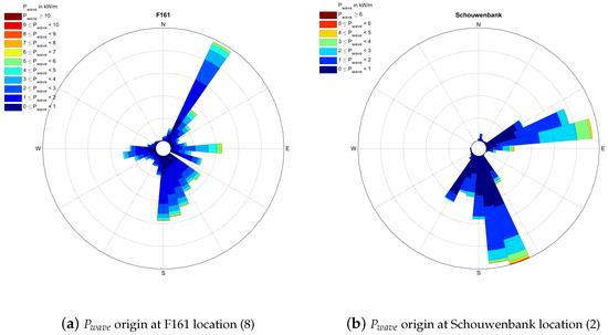
Figure 14.
at indicative Northern (a) and Southern (b) locations.
Supplementing the information necessary for any offshore activity, accessibility is an indicator of the time when conditions are favourable for operations. When maintenance and operation (M&O) is necessary, usually vessels and manned ships have to go at the location and perform repairs or investigation. These vessels depend on metocean conditions and usually can operate safely within a certain range of s. Vessels for M&O consider m [46,47]. Depending on the threshold for safe vessels sea-going, accessibility levels vary.
When the threshold is m, the accessibility at the most energetic (Northern provinces) is from 40–60%, as we move toward the Southern provinces accessibility slightly increases but does not exceed . Only regions in the inner canals, inlets and artificially made seaways have ≥90%. When the vessels employed are able to operate at 1.5 m, there is a significant increase in the accessibility. At Northern provinces, accessibility increases by 20–35%, with nearshore areas ≈75–85% and as the fetch increases accessibility values are ≈70%. As the regions of interest move Southward, accessibility levels rise significantly and are consistently ≥75% even at depths of ≥40 m, see Figure 15.
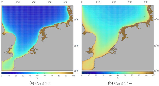
Figure 15.
Accessibility in percentage of time, based on different thresholds.
5. Discussion
The ST6 package allows re-computation of wind stress and local-cumulative dissipation terms and seems to enhance performance. Using wind drag formulation based on WAM 3 and WAM 4, mean values were over and under-estimated, respectively. With regards to WAM 4 wind drag hindcasts with a “peakier” performance, while WAM 3 consistently under-estimates. ST6 offers a “middle” ground solution; when properly tuned, dissipation can be adjusted to ensure not being turned to higher frequencies, allowing a better computation of low frequency (high period) waves. The developed model for the NSWD hindcast found that the most suitable configuration is based on adapting the Hwang wind drag coefficient, adopting dissipation terms according to option 2 and utilizing the re-computation of dissipation terms to minimise under-estimations. The scaling option had little effect, but a higher value allowed for better maxima reproduction. Moreover, it is highly advised to activate the linear growth as we noticed more under-estimates in the performance.
The model was modelled for 38 years and developed a comprehensive dataset with metocean conditions. It is often overlooked how important wave resource assessments are, and the level of intricacies they require to be considered. Especially, for extrapolation of resource characteristics and/or renewable energies, using datasets without appropriate considerations as per international peer-reviewed standards should be discouraged. Resource assessments have to be gradual and multi-levelled, as there is no perfect model. However, with detailed model calibration and validation, the assumptions can be minimised, and provide information which can quantify the uncertainty, giving confidence in any further analysis.
Resource assessment should also always consider the scope of study and potential use of their hindcast datasets. Depending on the application, several higher fidelity nested and multi-model analysis may be necessary. The current NSWD satisfies a two-fold purpose, firstly, it offers high-resolution information over the North Sea and has adequate spatio-temporal resolution to characterise the wave energy resource and identify hot-spots. Secondly, it also provides ample information on the metocean conditions that can be useful for many other offshore activities and constructions. Long-term homogenous datasets are key for the minimisation of cost in many offshore industries, as they allow for better estimation of forces on structures and accessibility and can ultimately reduce the over-size of components, thus leading to cost reductions.
6. Conclusions
Although we cannot expect that numerical wave models will be explicitly deterministic in their assessment, a major improvement has been introduced with this configuration. When also compared with other wind drag and dissipation parametrisations, it is observable that the bias is reduced, but most importantly, the highest waves are “captured”. For the calibration, several models and physical configurations were examined, with results similarly close. However, the configuration which was selected to construct the NSWD database showed a good level of consistency across the quantitative characteristics employed, the was high for all values examined and consistently around ≥98%. The NSWD managed to reduce mean under-estimations, and have a close agreement with maxima values, which are hugely important in the survivability of structures and are usually under-estimated significantly. Some locations showed an over-estimation of mean and maxima, though these locations are at regions where currents influence the wave resource, and since the NSWD model did not include such current information, it is advisable that higher resolution modelling is employed for these locations. Especially, the ones that are located in the outlets of estuaries. The biases trend indicated a close agreement with mostly a slight over-estimation that for all locations averaged 15 cm. Central and Northern parts of the Netherlands were better hindcasted and gave higher agreements with almost zero biases. Similarly, the configuration and tuning used for the NSWD reduced the under-estimation of maxima events within ±25–30 cm.
Subsequently, and after the comprehensive validation of the NSDW database, metocean conditions and statistical parameters were assessed to reveal most prevalent values. In terms of , Northern regions are exposed and influenced by swells from the Norwegian Sea having higher magnitudes with mean values being 1 m more than Southern regions, with values 5–6 and 4–5 m, respectively. In Northern provinces, the and indicate that the resource is usually 4 m and 6 s near the coastlines and at depths of ≥40 m it is ≈5 m and 8 s. At Central provinces, coastal regions such as Bergen and Leiden, the majority of values are slightly decreasing. The reductions are not sudden, with bottom-induced breaking to be “smoothed” by bathymetry of the continental shelf, providing constant - values at 3.5 m and 7 s, respectively. Towards the South, there is a small decreases due to lower exposure to swells and narrowing of the English channel, but magnitudes are similar to the Central coastlines. Further, away from the coast, at depths of ≥30 m, the resource shows similar trends as in the Northern regions.
Interestingly, variability as expressed by values is low for throughout the domain at nearshore, shallow and deeper regions with values in the range of ≈0.2–0.25. However, in the case of , there are moderate levels of expected variability, as in deeper water, the is ≈0.5, while at locations with depths ≤20 m and very coastal locations, the resource indicates minimal expected changes with values close to 0.2. This indicates that the wave energy flux, which is highly dependent on , will be affected and in an on-going study we aim to determine climate persistence effects, therefore, identifying resource trends.
NSWD is the first database of high-fidelity metocean conditions that also examined the wave energy content for the region. The North Sea is considered of low energy, however, the mean energy flux indicates that there is more energy content, and it is highly accessible. At Northern parts of the NSWD domain, both for the United Kingdom and the Netherlands, depths are ≤60 m and have an energy flux of 15–20 kW/m. Closer to the English channel, resource potential drops significantly due to orography interactions of the straits and coastal influences, with energy content reduced to 3–6 kW/m. In terms of wave energy, interesting regions are the Northern provinces, including the Wadden and Texel islands, which have a of 8–20 kW/m at low depths where WECs can bpotentiale deployed cost-effectively and benefit from high vessels accessibility ≥90%. In the United kingdom, at the Norwich and Ipswich coasts is ≤4 kW/m, but exactly across the Central and South Dutch coastlines these have a significant resource of ≥10 kW/m.
Although, not energetic as coastlines of the Irish Republic and Scotland, the North Sea benefits from good levels of wave energy resource. Wave energy converters should not only be considered for high energy resources, on the contrary, milder and moderate resources offer better potential. An added advantage of the North Sea region, are the “slow” gradients and change in bathymetry which significantly influences wave energy content. Even at very close proximity to the shore and depths from 20 m, is significant ≥7 kW/m and can arguably foster the development of ocean wave energies.
Although numerical modelling has its limitations, it is a “powerful" tool that provides information vital to reduce assumptions, especially for offshore energies, structures and performance evaluation. To that end, reliable databases are vital for any future development. When considering reliability, we should expect that there will not be a total agreement, but rather we should seek to improve the databases produced by elaborating on physical configuration and performance limitations. Knowing the limitation of each solution provides valuable information and confidence in the use of any subsequent database. The NSWD has shown a very good agreement with higher values at the Northern parts, indicating that the nearshore and swell interactions are resolved. Due to the scale NSWD’s first layer, very shallow locations show a small reduction in accuracy. Influence of currents reduce the wave resource at very nearshore areas, and influence their potential variance, indicating that further nesting is necessary. Nevertheless, NSWD offers significant information and addresses the lack of quantifiable metocean and wave power assessment for the North Sea region, revealing that the level of wave energy is higher than anticipated.
Author Contributions
Conceptualization, definition, model development and parametrisation was done by G.L. The writing and review was performed by G.L., suggestions and comments were provided by H.P.
Funding
The first author (Research Fellow) and WAVe Resource for Electrical Production (WAVREP) project has received funding from the European Union’s Horizon 2020 research and innovation programme under the Marie Skłodowska-Curie grant agreement No 787344.
Acknowledgments
We would like to thank the reviewers for their time, comments and suggestions, that helped use improve the quality of the manuscript.
Conflicts of Interest
The authors declare no conflict of interest.
Abbreviations
The following abbreviations are used in this manuscript:
| Exponential growth | |
| wave steepness coefficient | |
| direction | |
| longitude | |
| Water density | |
| angular frequency | |
| latitude | |
| Non-dimensional Wind | |
| A | linear growth |
| c | energy propagation |
| wind drag coefficient | |
| cumulative dissipation | |
| centimetres | |
| Coefficient of Variation | |
| CSN | Climatological Standard Normals |
| Mean wave direction | |
| E | action density |
| f | frequency |
| Significant wave height | |
| Maximum significant wave height | |
| g | gravitational acceleration |
| local dissipation | |
| m | Meters |
| Maintenance and operation | |
| MPI | Model Performance Index |
| NWM | Numerical Wave Models |
| Peak wave direction | |
| Percentile value | |
| R | Correlation coefficient |
| Root Mean Square Error | |
| Observed changes | |
| , s | seconds |
| Scatter Index | |
| wind input | |
| triads | |
| Quadruplet interactions | |
| Whitecapping | |
| bottom friction | |
| depth breaking | |
| t | time |
| Mean Zero Crossing period | |
| Average wave period | |
| Maximum of average wave period | |
| wave energy converters | |
| Wind speed at 10 meter height | |
| Reference Wind |
References
- Caires, S.; Groeneweg, J.; Sterl, A. Past and Futures Changes in the North Sea Extreme Waves. ICCE 2008, 19, 7666. [Google Scholar]
- Lavidas, G.; Agarwal, A.; Venugopal, V. Marine Activities Dependence on Offshore Climatic Conditions. In Energy in Transportation (EinT), ASHRAE; Deligkiozi, I., Ed.; ASHRAE: Athens, Greece, 2016; pp. 29–36. [Google Scholar]
- Agarwal, A. A Long-Term Analysis of the Wave Climate in the North East Atlantic and North Sea. Ph.D. Thesis, University of Edinburgh, Edinburgh, UK, 2015. [Google Scholar]
- Reguero, B.; Losada, I.J.; Mendez, J.F. A recent increase in global wave power as a consequence of oceanic warming. Nat. Commun. 2019, 1–14. [Google Scholar] [CrossRef] [PubMed]
- Chawla, A.; Spindler, D.M.; Tolman, H.L. Validation of a thirty year wave hindcast using the Climate Forecast System Reanalysis winds. Ocean. Model. 2013, 70, 189–206. [Google Scholar] [CrossRef]
- Reguero, B.; Losada, I.; Méndez, F. A global wave power resource and its seasonal, interannual and long-term variability. Appl. Energy 2015, 148, 366–380. [Google Scholar] [CrossRef]
- Caires, S.; Sterl, A. 100-year return value estimates for ocean wind speed and significant wave height from the ERA-40 data. J. Clim. 2005, 18, 1032–1048. [Google Scholar] [CrossRef]
- Galanis, G.; Chu, P.C.; Kallos, G.; Kuo, Y.H.; Dodson, C.T.J. Wave height characteristics in the north Atlantic ocean: A new approach based on statistical and geometrical techniques. Stoch. Environ. Res. Risk Assess. 2012, 26, 83–103. [Google Scholar] [CrossRef]
- Bailey, B.H.; McDonald, S.L.; Bernadett, D.W.; Markus, M.J.; Elsholz, K.V. Wind Resource Assessment Handbook: Fundamentals for Conducting a Successful Monitoring Program; Technical Report; National Renewable Energy Laboratory (NREL): Golden, CO, USA, 1997.
- World Bank. Best Practice Guidelines for Mesoscale Wind Mapping Projects for the World Bank; Technical Report; World Bank: Washington, DC, USA, 2010. [Google Scholar]
- Ingram, D.; Smith, G.H.; Ferriera, C.; Smith, H. Protocols for the Equitable Assessment of Marine Energy Converters; Technical Report; Institute of Energy Systems, University of Edinburgh, School of Engineering: Edinburgh, UK, 2011. [Google Scholar]
- Smith, H.; Maisondieu, C. Resource Assessment for Cornwall, Isles of Scilly and PNMI; Technical Report; University of Exeter and Ifremer: Exeter, UK, 2014. [Google Scholar]
- Lavidas, G.; Venugopal, V.; Friedrich, D. Wave energy extraction in Scotland through an improved nearshore wave atlas. Int. J. Mar. Energy 2017, 17, 64–83. [Google Scholar] [CrossRef]
- World Meteorological Organization. WMO Guidelines on the Calculation of Climate Normals; Technical Report; World Meteorological Organization: Geneva, Switzerland, 2017. [Google Scholar]
- Cavaleri, L.; Sclavo, M. The calibration of wind and wave model data in the Mediterranean Sea. Coast. Eng. 2006, 53, 613–627. [Google Scholar] [CrossRef]
- Vinoth, J.; Young, I.R. Global Estimates of Extreme Wind Speed and Wave Height. J. Clim. 2011, 24, 1647–1665. [Google Scholar] [CrossRef]
- Cavaleri, L.; Bertotti, L.; Pezzutto, P. Accuracy of altimeter data in inner and coastal seas. Ocean Sci. 2019, 15, 227–233. [Google Scholar] [CrossRef]
- WAMDI, G. The WAM Model-a Third Generation Ocean Wave Prediction Model. Phys. Oceanogr. 1988, 18, 1775–1810. [Google Scholar]
- Lavidas, G.; Venugopal, V. Application of numerical wave models at European coastlines: A review. Renew. Sustain. Energy Rev. 2018, 92, 489–500. [Google Scholar] [CrossRef]
- Rijkswaterstaat. Ministry of Infrastructure and Water Management. Available online: https://www.rijkswaterstaat.nl (accessed on 21 March 2019).
- Larsén, X.G.; Kalogeri, C.; Galanis, G.; Kallos, G. A statistical methodology for the estimation of extreme wave conditions for offshore renewable applications. Renew. Energy 2015, 80, 205–218. [Google Scholar] [CrossRef]
- Dodet, G.; Bertin, X.; Taborda, R. Wave climate variability in the North-East Atlantic Ocean over the last six decades. Ocean Model. 2010, 31, 120–131. [Google Scholar] [CrossRef]
- Delft, T. SWAN Scientific and Technical Documentation Cycle III Version 41.01; Technical Report; Delft University of Technology: Delft, The Netherlands, 2014. [Google Scholar]
- Amante, C.; Eakins, B. ETOPO1 1 Arc-Minute Global Relief Model: Procedures, Data Sources and Analysis; NOAA Technical Memorandum NESDIS NGDC-24; NOAA: Silver Spring, MD, USA, 2014. [Google Scholar]
- Wessel, P.; Smith, W.H.F. A Global Self-consistent, Hierarchical, High-resolution Shoreline Database. J. Geophys. Res. 1996, 101, 8741–8743. [Google Scholar] [CrossRef]
- Dee, D.P.; Uppala, S.M.; Simmons, A.J.; Berrisford, P.; Poli, P.; Kobayashi, S.; Andrae, U.; Balmaseda, M.A.; Balsamo, G.; Bauer, P.; et al. The ERA-Interim reanalysis: Configuration and performance of the data assimilation system. Q. J. R. Meteorol. Soc. 2011, 137, 553–597. [Google Scholar] [CrossRef]
- Akpinar, A.; Ponce de León, S. An assessment of the wind re-analyses in the modelling of an extreme sea state in the Black Sea. Dyn. Atmos. Ocean. 2016, 73, 61–75. [Google Scholar] [CrossRef]
- Stopa, J.E.; Cheung, K.F. Intercomparison of wind and wave data from the ECMWF Reanalysis Interim and the NCEP Climate Forecast System Reanalysis. Ocean. Model. 2014, 75, 65–83. [Google Scholar] [CrossRef]
- Lavidas, G.; Venugopal, V.; Friedrich, D. Sensitivity of a numerical wave model on wind re-analysis datasets. Dyn. Atmos. Ocean. 2017, 77, 1–16. [Google Scholar] [CrossRef]
- Agarwal, A.; Venugopal, V.; Harrison, G.P. The assessment of extreme wave analysis methods applied to potential marine energy sites using numerical model data. Renew. Sustain. Energy Rev. 2013, 27, 244–257. [Google Scholar] [CrossRef]
- National Oceanic and Atmospheric Administration (NOAA), WaveWatchIII. Available online: https://polar.ncep.noaa.gov/waves/wavewatch/ (accessed on 14 September 2019).
- Ponce de León, S.; Bettencourt, J.; Van Vledder, G.P.; Doohan, P.; Higgins, C.; Guedes Soares, C.; Dias, F. Performance of WAVEWATCH-III and SWAN Models in the North Sea. In Proceedings of the 37th International Conference on Ocean, Madrid, Spain, 17–22 June 2018. [Google Scholar] [CrossRef]
- Kamranzad, B.; Mori, N. Future wind and wave climate projections in the Indian Ocean based on a super-high-resolution MRI-AGCM3.2S model projection. Clim. Dyn. 2019. [Google Scholar] [CrossRef]
- Rogers, W.E.; Babanin, A.V.; Wang, D.W. Observation-Consistent Input and Whitecapping Dissipation in a Model for Wind-Generated Surface Waves: Description and Simple Calculations. J. Atmos. Ocean. Technol. 2012, 29, 1329–1346. [Google Scholar] [CrossRef]
- Komen, G.; Hasselmann, S.; Hasselmann, K. On the Existence of a Fully Developed Wind-Sea Spectrum.pdf. Phys. Oceanogr. 1984, 14, 1271–1285. [Google Scholar] [CrossRef]
- Janssen, P.A. Quasi-Linear theory of Wind-Wave Generation applied to wave forecasting. J. Phys. Oceanogr. 1991, 6, 1631–1642. [Google Scholar] [CrossRef]
- van der Westhuysen, A.J.; Zijlema, M.; Battjes, J. Nonlinear saturation-based whitecapping dissipation in SWAN for deep and shallow water. Coast. Eng. 2007, 54, 151–170. [Google Scholar] [CrossRef]
- Zieger, S.; Babanin, A.V.; Erick Rogers, W.; Young, I.R. Observation-based source terms in the third-generation wave model WAVEWATCH. Ocean Model. 2015. [Google Scholar] [CrossRef]
- Hwang, P.A. A Note on the Ocean Surface Roughness Spectrum. J. Atmos. Ocean. Technol. 2011, 28, 436–443. [Google Scholar] [CrossRef]
- Fan, Y.; Lin, S.J.; Held, I.M.; Yu, Z.; Tolman, H.L. Global Ocean Surface Wave Simulation Using a Coupled Atmosphere–Wave Model. J. Clim. 2012, 25, 6233–6252. [Google Scholar] [CrossRef]
- Ardhuin, F.; Rogers, E.; Babanin, A.V.; Filipot, J.F.; Magne, R.; Roland, A.; van der Westhuysen, A.; Queffeulou, P.; Lefevre, J.M.; Aouf, L.; et al. Semiempirical Dissipation Source Functions for Ocean Waves. Part I: Definition, Calibration, and Validation. J. Phys. Oceanogr. 2010, 40, 1917–1941. [Google Scholar] [CrossRef]
- Janssen, P.A. Wave-induced Stress and drag of air flow over sea waves. J. Phys. Oceanogr. 1988, 19, 745–754. [Google Scholar] [CrossRef]
- Zijlema, M.; van Vledder, G.P.; Holthuijsen, L. Bottom friction and wind drag for wave models. Coast. Eng. 2012, 65, 19–26. [Google Scholar] [CrossRef]
- Rijkswaterstaat. Open Data Rijkswaterstaat Waterdienst. 2018. Available online: https://bignieuws.nl/open-data-rijkswaterstaat/ (accessed on 10 February 2019).
- Lavidas, G. Wave Energy Resource Modelling and Energy Pattern Identification Using a Spectral Wave Model. Ph.D. Thesis, University of Edinburgh, School of Engineering, Edinburgh, UK, 2016. [Google Scholar]
- Katsouris, G.; Savenije, L.B. Offshore Wind Access 2017; Technical Report December 2016; Energy Centre Netherlands (ECN): Petten, The Netherlands, 2017. [Google Scholar]
- Lavidas, G.; Agarwal, A.; Venugopal, V. Availability and Accessibility for Offshore Operations in the Mediterranean Sea. J. Waterw. Port Coast. Ocean. Eng. 2018, 144, 1–13. [Google Scholar] [CrossRef]
© 2019 by the authors. Licensee MDPI, Basel, Switzerland. This article is an open access article distributed under the terms and conditions of the Creative Commons Attribution (CC BY) license (http://creativecommons.org/licenses/by/4.0/).