Wind Stress in the Coastal Zone: Observations from a Buoy in Southwestern Norway

Abstract

Several studies have focused on the investigation of the wind stress in open ocean conditions where coastal processes were negligible. However, the direction and magnitude of the wind stress vector in coastal areas are still not fully known due to the low number of available measurement datasets. Here, we present new observations of the wind stress magnitude and its deviation from the mean wind direction. The data were recorded from a surface buoy during a five-day measurement campaign in southwestern Norway and cover wind speeds up to 10 m s⁻¹ and significant wave heights up to 3.5 m in a coastal area with a steeply sloping sea floor. The adjustment of the wind stress vector due to changes in the wind and the wave conditions is illustrated and discussed by means of seven sample cases associated with both wind-following swell, cross-swell and counter-swell conditions. For this purpose, the stress vector computed in the sonic anemometer’s orthogonal coordinate system is projected into a non-orthogonal wind-swell coordinate system with its components aligned with: (1) the local wind-generated waves propagating in the wind direction; and (2) the swell wave direction. The wind stress direction was found to deviate from the wind direction by more than 20° for 46% of the recorded wind-following swell and cross-swell cases and for 54% of the counter-swell cases. The wind stress magnitude was observed to approach zero during the counter-swell period, which suggest a decoupling between the sea surface and the atmospheric surface layer. This was further investigated by means of an idealized Large Eddy Simulation results. The results in this study provide additional experimental evidence that the wind stress direction in coastal areas with a steeply sloping sea floor is influenced by the swell waves, the wave age and the wave steepness when the wind blows from undisturbed open ocean directions. For landward wind directions, the influence of the land boundary layer can, possibly in combination with atmospheric stability, adjust the magnitude and direction of the wind stress.

1. Introduction

Winds blowing over the ocean exert a forcing on the air–sea interface. As a response to the wind forcing, short surface gravity waves form at the sea surface, which increase the surface roughness and thus the wind stress and the wave height. The feedback between the wind forcing and the wave growth, i.e., the increase in sea surface roughness and wind stress, continues until the waves have reached an equilibrium with the wind forcing [1,2]. The magnitude of the wind stress on the sea surface governs the exchange of horizontal momentum between the atmosphere and the ocean, which is a key process to drive the coupled atmosphere–ocean system. Understanding the adjustment of the wind stress to the wind and wave forcing is thus crucial as it contributes to processes that govern the global climate system through the exchange of momentum, heat and gas across the air–sea interface. While the wind stress direction and the wind direction are mostly concurrent over land, wind stress measurements over the ocean have revealed differences between both directions. Numerous studies have investigated the wind stress and the associated exchange of vertical momentum flux over the ocean during the last decades. Analyzing wind stress measurements recorded at a Light Tower off the coast of Virginia, Geernaert et al. [3] found evidence that the stress vector direction turns towards the propagation direction of the swell waves during the presence of light winds and near-zero heat flux. This finding was further supported by Rieder et al. [4] and Rieder and Smith [5] who analyzed wind stress and wave data collected from aboard RP FLIP at two locations off the US west coast. They observed a turning of the stress vector towards the propagation direction of the swell waves for wind speeds up to 12 m s⁻¹. Investigating wind stress data collected during the San Clemente Ocean Probing Experiment (SCOPE), Grachev and Fairall [6] observed a counter-clockwise turning of the stress vector with decreasing wind speed in wind-following swell conditions. They reported a 180° turning of the stress vector direction relative to the wind direction for wind speeds smaller than 2 m s⁻¹. These weak wind cases were further associated with a positive vertical momentum flux and thus an upward transport of horizontal momentum, i.e., from the ocean to the atmosphere.

In recent years, the investigation of the wind stress vector magnitude and direction in coastal areas has received increased attention. These areas are characterized by a variety of interlinked processes that are expected to influence the wind stress, such as wave shoaling, wave refraction and wave breaking, coastal surface currents and internal boundary layers. Zhang et al. [7] investigated the interaction between coastal surface currents, the wave field and the stress vector direction by means of Ocean Surface Current Radar and the use of several ASIS buoys that were moored off the coast of North Carolina. They found that peak period waves were refracted away from the mean wind direction when winds were blowing across a strong surface current vorticity field, while waves which have reached equilibrium with the wind were observed to propagate into the mean wind direction. They further reported that the directional change of the most energetic waves led to the development of an off-wind stress component, the magnitude of which corresponded to the upwind vorticity field. Shabani et al. [8] performed wind stress measurements over waves within the surf zone from two sonic anemometers mounted at heights of 5 and 10 m above the water surface at an open beach in eastern Australia. For near-neutral atmospheric conditions, they found the drag coefficient (wind stress) to vary with the wind angle of approach relative to the shoreline. For onshore winds, i.e., winds blowing from the sea towards the land, they reported drag coefficients of twice the values as for open ocean conditions. The increased wind stress in the surf zone was attributed by Shabani et al. [8] to a decrease in wave celerity combined with a change in the wave shape (i.e., wave shoaling). Ortiz-Suslow et al. [9] performed eddy covariance measurements in a river inlet in North Carolina to evaluate the suitability of wind speed dependent wind stress parameterizations in coastal areas. They observed a deviation of the wind stress direction from the mean wind direction within the river inlet and up to 2 km offshore. They further observed the stress vector deviation to be correlated with the horizontal current shear, and concluded that open ocean parameterizations underestimate the drag coefficient by a factor of 2.6. Recently, Ortiz-Suslow et al. [10] observed a shift from swell- to current-dominated wind stress veering at a distance of 2 km off the coast in Monterey Bay, California. They reported a relationship between the wind stress veering and the alongshore surface current variance, within 2 km off the coast. At distances further offshore, the wind stress veering was found to be constant and attributed to the influence of the swell wave field.

Grachev et al. [11] performed eddy-covariance measurements at four met-towers that were located at subsequent landward distances from the shoreline. Although this study mainly focused on the applicability of the Monin–Obukhov Similarity Theory in the coastal zone, their results highlight the variety of different turbulent flux footprints which exist over the land transition zone. For example, they observed drag coefficients associated with land-footprints to be an order of magnitude higher than drag coefficients associated with sea-footprints, resulting from differences in the surface roughness between the land and the sea surface. The variety of flux-footprints in the coastal zone can lead to the development of an internal boundary layer which modifies the wind stress within the lower part of the atmosphere due to advection and the consecutive divergence or convergence of vertical momentum flux (e.g., Mahrt et al. [12] and Mahrt et al. [13]).Despite increased efforts to accurately determine the turbulent momentum fluxes in coastal areas, the modification of the wind stress due to interlinked coastal processes is still not fully understood and resolved in atmosphere–ocean models. The uncertainties embedded in modelled wind stress lead to imprecise estimations of the global energy balance, which highly affects the global climate system [14]. To further improve our current understanding of the wind stress close to the sea surface, and thus the horizontal transfer of momentum across the wavy air–sea interface, measurements of momentum and heat fluxes at different locations around the world are highly needed. For example, the World Climate Research Program (WCRP) Surface Flux Task Team [15] encourages the acquisition of eddy-covariance flux measurements in locations and conditions that are currently not well represented in the existing literature and datasets (see, Clayson et al. [14]).

This paper presents observations of the wind stress vector magnitude and the deviation of the wind stress from the mean wind direction. The measurements of the wind stress, i.e., the vertical momentum flux, were performed from a surface buoy at an altitude of approximately 4 m above sea level and cover wind speeds up to 10 m s⁻¹ and significant wave heights up to 3.5 m in a coastal area with a steeply sloping sea floor. The adjustment of the wind stress vector due to changes in the wind and the wave conditions is illustrated and discussed by means of seven sample cases associated with both wind-following swell, cross-swell and counter-swell conditions. The results of an idealized Large Eddy Simulation that was conducted to investigate the onset of a land-breeze resulting from the temperature difference between colder land and warmer sea are also presented. With its measurement location in southwestern Norway, this paper provides a new dataset for an area with rather complex coastal features, thus far not represented in the literature.

The methodology applied for the derivation of the wind stress magnitude and direction is described in Section 2. The experimental set-up, the environmental conditions during the deployment period and an overview of the data processing is described in Section 3. Section 4 presents the results and the discussion, while Section 5 provides a short summary and outlook.

2. Methodology

The interaction of the waves with the atmosphere leads to the formation of a wave boundary layer (WBL) between the sea surface and the lower part of the atmospheric boundary layer, in which the influence of the waves on the stress vector cannot be neglected [16]. Within the WBL, the wind velocity components are a superposition of mean, turbulent and wave-induced parts and can be written as

$$\mathbf{u}=\overline{\mathbf{u}}+{\mathbf{u}}^{\prime }+\tilde{\mathbf{u}},$$

(1)

where $\mathbf{u}=(u,v,w)$ denotes the velocity vector in which u and v are the horizontal velocity components and w the vertical velocity component. The notations ($\overline{\phantom{u}}$), (${}^{\prime }$) and ($\tilde{\phantom{u}}$) are operators denoting the mean, the turbulent and the wave-induced parts of the wind velocity vector, respectively. The stress vector $\mathbf{\tau }$ is commonly determined from sonic anemometer measurements by means of the eddy-covariance method, i.e.,

$$\mathbf{\tau }=-\rho \langle u^{\prime }{w}^{\prime }+\tilde{u}\tilde{w}\rangle \mathbf{i}-\rho \langle v^{\prime }{w}^{\prime }+\tilde{v}\tilde{w}\rangle \mathbf{j}={\mathbf{\tau }}_x+{\mathbf{\tau }}_y,$$

(2)

where $\rho$ denotes the air density, the brackets $\langle \rangle$ denote a time-average mean and $\mathbf{i}$ and $\mathbf{j}$ represent the longitudinal and lateral unit vectors, respectively. The wave-induced fluctuations are expected to decrease exponentially with height [17,18,19] and the wind stress outside the WBL is thus only supported by the turbulent fluctuations around the mean values of the wind speed components. The deviation of the wind stress direction from the wind direction, i.e., the off-wind angle, is correspondingly determined as

$$\alpha ={tan}^{-1}(\langle v^{\prime }{w}^{\prime }+\tilde{v}\tilde{w}\rangle /\langle u^{\prime }{w}^{\prime }+\tilde{u}\tilde{w}\rangle ).$$

(3)

According to Grachev et al. [20], Equation (2) can be written as follows

$$\begin{array}{cc}\hfill {\tau }_1& ={\tau }_x-{\tau }_{y}cot\theta \mathrm{and}{\tau }_2={\tau }_y/sin\theta ,\hfill \end{array}$$

(4)

where $\mathbf{\tau }={\mathbf{\tau }}_1+{\mathbf{\tau }}_2$ in which ${\tau }_1$ and ${\tau }_2$ are the wind stress along the wind-wave and wind-swell directions, and $\theta$ is the relative angle between the wind and the swell wave propagation direction. Equation (4) projects the components of the wind stress vector from an orthogonal wind vector based coordinate system onto a non-orthogonal wind-swell based coordinate system. A schematic representation of the stress vector decomposition in both coordinate systems is shown in Figure 1. Since ${\mathbf{\tau }}_{\mathbf{2}}$ is assumed to be aligned with the swell waves (in the same or opposite propagation direction), the use of this approach is limited to swell dominated seas and mixed seas with background swell. We point out that the conversion of the stress vector components between the two coordinate systems depends on the relative angle between the wind and the swell wave propagation direction. Therefore, the applicability of this approach breaks down for cases where the wind direction is aligned with, or opposite to, the swell wave propagation direction, i.e., $\theta \approx 0$.

The total net-transport of momentum across the air–sea interface can also be expressed as the sum of the shear stress ${\mathbf{\tau }}_s$ and the wave-induced stress $\tilde{\mathbf{\tau }}$, i.e.,

$$\mathbf{\tau }={\mathbf{\tau }}_s+\tilde{\mathbf{\tau }}={\mathbf{\tau }}_{visc}+{\mathbf{\tau }}^{\prime }+\tilde{\mathbf{\tau }},$$

(5)

where the shear stress is composed of the viscous stress ${\mathbf{\tau }}_{visc}$ and the turbulent stress ${\mathbf{\tau }}^{\prime }$. At the sea surface, the turbulent stress is negligible and the total stress can be approximated as the sum of the viscous stress and the wave-induced stress [20,21]. Although the shear stress has both longitudinal and lateral components, its direction is approximately aligned with the mean wind direction [20].

Swell waves are generated by distant low-pressure systems and their propagation direction is not influenced by local winds. In contrast, the propagation direction of the locally wind-generated waves is governed by the local wind direction. By assuming that there is no correlation between wind-generated and swell waves, the wave-induced stress at the sea surface can be approximated as

$$\tilde{\mathbf{\tau }}=\widetilde{{\mathbf{\tau }}_1}+\widetilde{{\mathbf{\tau }}_2}.$$

(6)

where $\widetilde{{\mathbf{\tau }}_1}$ and $\widetilde{{\mathbf{\tau }}_2}$ are components aligned with the locally wind-generated waves and the swell wave direction. Although the wave field often consists of locally wind-generated waves with different wave periods that travel in slightly different directions, it is reasonable to hypothesize that the majority of the short waves approximately propagate in the mean wind direction (cf. Masson [22]).

Accordingly, the stress vector components ${\mathbf{\tau }}_1$ and ${\mathbf{\tau }}_2$ can also be written using the shear stress and the wave-induced stresses as follows,

$$\begin{array}{c}\hfill {\mathbf{\tau }}_1\approx {\mathbf{\tau }}_s+\widetilde{{\mathbf{\tau }}_1}\mathrm{and}{\mathbf{\tau }}_2\approx \widetilde{{\mathbf{\tau }}_2}.\end{array}$$

(7)

We use a left-handed coordinate system in this study and have rotated the recorded wind velocities into the streamwise wind. The longitudinal wind component is related to the along-wind stress, i.e., ${\tau }_x\mathbf{i}\equiv -\rho \langle u^{\prime }{w}^{\prime }+\tilde{u}\tilde{w}\rangle \mathbf{i}$, which is defined as positive when ${\tau }_x\mathbf{i}$ is facing into the along-wind direction. The lateral stress component, i.e., the cross-wind stress ${\tau }_y\mathbf{j}\equiv -\rho \langle v^{\prime }{w}^{\prime }+\tilde{v}\tilde{w}\rangle \mathbf{j}$, is defined as positive (negative) if it is directed to the right (left) of the wind vector. Off-wind angles derived from Equation (3) are positive (negative) when the stress vector is orientated to the right (left) of the wind vector. For the remainder of this paper, the notation (${}^{\prime }$) is used to represent both the turbulent and wave-induced parts of the vertical momentum fluxes.

The sign and magnitude of ${\mathbf{\tau }}_1$ and ${\mathbf{\tau }}_2$ are governed by a combination of the wind speed and the sea state. The phase speed of short locally wind-generated waves ($c_p$) is typically lower than the wind speed (U) so that the short waves act as roughness elements that extract horizontal momentum from the atmosphere, i.e., ${\tau }_1>0$. The case ${\tau }_1<0$ is associated with decaying wind conditions where the wind speed quickly decreases below the phase speed of the short locally wind-generated waves [20]. In this situation, wave-induced pressure perturbations generate a pressure drag on the atmosphere which leads to upward transfer of wave-induced horizontal momentum into the atmospheric surface layer. The situation is similar for swell waves, where ${\tau }_2>0$ when the swell propagates into the wind direction during moderate to strong winds (cf. Grachev and Fairall [6], Sullivan et al. [23,24]). The magnitude of ${\mathbf{\tau }}_2$ decreases with decreasing wind speed. It is expected that ${\mathbf{\tau }}_2$ becomes negative in conditions where fast swell waves propagate into the wind direction during low winds, e.g., typically $U<2$ m s⁻¹ and wave age $c_p/U>2.5$ [25]. In these situations, wave-induced momentum is transferred from the ocean to the atmosphere (cf. Grachev and Fairall [6], Babanin et al. [19], Högström et al. [26]). In counter-swell situations, the wind drags against the waves, i.e., ${\tau }_2<0$, and momentum is extracted from the atmosphere (cf. Donelan et al. [27], Kudryavtsev and Makin [28]). The exchange of horizontal momentum from the atmosphere to the ocean, i.e., downward directed vertical momentum flux, occurs when the net wind stress is positive ($\tau >0$) [20].

Commonly, the wind stress magnitude and wind stress direction close to the sea surface are extrapolated from the sonic anemometer measurements performed at a certain height, e.g. 10 m, by assuming that the height variation of the turbulent fluctuations in Equation (2) is negligible within the atmospheric surface layer. Moreover, the wave-induced fluctuations in Equation (2) are typically neglected, as many studies assume that their eddy-covariance measurements were performed outside the wave boundary layer. However, this approach might fail to provide accurate surface stress estimates due to advection of vertical momentum flux and consecutive changes in the surface layer wind stress (cf. Mahrt et al. [12,13] Babanin et al. [19], Hare et al. [29], Miller [30]). Revisiting data from several offshore measurement campaigns, Mahrt et al. [13] noted that the vertical momentum flux, i.e., the wind stress magnitude, decreases (increases) with height over the open ocean (in coastal areas) due to momentum flux divergence (convergence). They concluded that the wind stress magnitude close to the sea surface needs to be extrapolated from eddy-covariance measurements performed at several levels above the sea surface. However, Mahrt et al. [13] also found indications that the height variations of the momentum flux might be negligible up to heights ranging between 2 and 8 m above the sea surface, depending on site specific conditions. The data presented in this study were recorded from a sonic anemometer mounted on top of a buoy, approximately 4 m above the sea surface (see, Section 3.1). As we only have one measurement level, an extrapolation of the wind stress magnitude, such as proposed by Mahrt et al. [13], cannot be performed. Given the relatively small vertical distance between the measurement height and the sea surface for the present dataset, we find it, however, reasonable to treat the stress vector computed with Equation (2) as invariant with height.

3. Data Set

3.1. Buoy Deployment Site and Measurement Set-Up

To investigate the behavior of the wind stress vector for a variety of wind-wave conditions, a surface buoy was deployed approximately 1.2 km off the islet Kvernholmen between 23 and 29 November 2013. Kvernholem is located at the southwestern part of Sotra Island, nearby Marstein Fyr, 30 km southwest of Bergen, Norway (Figure 2).

Common for the southwest coast of Norway, the area in the vicinity of the deployment site consists of several small islets with rough rocky terrain and steep topography with an altitude of 20–30 m. The highest point of the southern part of Sotra Island rises 285 m above sea level and is located 9 km east of the deployment site. The buoy’s mooring site was located over a small 320 m × 350 m wide, submerged sea mountain, at a water depth ranging 40–50 m. The water depth around the sea mountain is approximately 50 m. Moreover, the mooring site is located in the coastal zone where the bathymetry is steeply increasing from a water depth of 300 m to sea surface level within a longitudinal distance of approximately 11 km (Figure 2). Waves approaching the mooring site have a westerly fetch of 330 km towards the Faroe Islands and a 1000–2300 km northwesterly to northerly fetch towards Iceland and Greenland, respectively.

The surface buoy used in the campaign was a commercially available Fugro Oceanor Seawatch Wavescan buoy that was developed for optimized wave direction measurements in addition to current and wave height measurements in severe environmental conditions. The buoy is discus shaped and has a diameter of 2.8 m. A well in the center of the buoy contains the batteries, the buoy’s data logger and a tailor-made wave sensor. The buoy performs wave direction measurements based on the heave/slope measuring principle. In addition, the buoy has a 3.5 m high mast that is by default equipped with an air temperature and humidity sensor, a propeller anemometer or a 2D sonic anemometer and GPS and communication antennae. Data collected by the buoy’s standard sensors (i.e., current direction, current speed, water and air temperature, and relative humidity) were continuously collected and averaged over 1 h. Wave direction, peak period and significant wave height were estimated by an internal algorithm of the buoy’s data processing unit that involves spectral analysis of one-hourly high frequency heave and tilt time series.

For the purpose of the campaign, the wind sensor and the antennae were removed from the buoy’s mast and replaced by a Gill R3-100 sonic anemometer and a Crossbow NAV440 inertial measurement unit (IMU). The IMU was placed in a watertight housing and attached to the buoy’s mast at a measurement height of approximately 3 m above the sea surface. The sonic anemometer was placed collinear on top of the IMU housing so that the anemometer measurement volume was centered approximately 4 m above the sea surface. The data logger for the sonic anemometer and the IMU was located inside a watertight enclosure that was attached on top of the buoy’s well.

The sonic anemometer measured the three dimensional wind vector, while the IMU provided the corresponding Euler attitude angles (i.e., roll, pitch and yaw), as well as wave-induced angular and translational velocities and buoy drift. Both instruments were measuring in a right-handed coordinate frame and continuously operated with a sampling frequency of 50 Hz. The anemometer’s and the IMU’s x-axes were pointing forward towards the buoy’s bow and were aligned with the buoy’s major axis, which runs along the line between the buoy center and the mast (i.e., towards the buoy’s north point). The corresponding y- and z-axes were pointing to the starboard side of the buoy and upward, respectively. The Wavescan buoy was equipped with a small vane beneath its south side to orientate the buoy’s major axis into the direction of the current. However, it was observed that the current vane was not sufficient to govern the orientation of the buoy. In fact, the major axes of the buoy, the sonic anemometer and the IMU were turned downwind during most of the campaign. The analysis of the sonic anemometer’s horizontal wind vector components revealed that the 20-min mean values of the offset angle between the major axis of the sonic anemometer relative to the downstream wind direction was within ± 12° for 63% and ± 22° for 71% of the data runs presented in this paper. For the remaining data, the offset angle was found to range form −117° to 84°. We believe that the orientation of the buoy relative to the wind was a combination of the current vane response to the prevailing surface currents and the wind torque created by both the enclosure mounted on top of the buoy’s well and the IMU housing. In addition to the IMU and sonic anemometer, a Campbell scientific CC5MPX digital network camera was mounted on top of the buoy’s mast rack to record sea surface gravity waves and whitecapping events. The analysis and discussion of the camera recordings is beyond the scope of this paper and the reader is referred to the work of Bakhoday-Paskyabi et al. [31].

3.2. Environmental Conditions

Various wind and wave conditions were encountered during the course of the campaign. The time series of the wind speed, wind direction and air temperature recorded approximately 4 m above the sea surface are shown in Figure 3. To relate these measurements to the overall weather condition around the deployment site, corresponding time series from three automated meteorological stations operated by the Norwegian meteorological institute are also shown in this figure. Two of the met-stations are located near to shore at Fedje Island, approximately 68 km north of the deployment site, and at Slåtterøy Island, approximately 31 km south of the deployment site. The met-station at the Gullfaks C oil platform in the North Sea is located approximately 185 km northwest of the deployment site and situated about 140 km offshore.

From noon on 23 November, the west coast of Norway was under the influence of a high-pressure system centered over Ireland, which led to a northerly wind field at the deployment site that persisted for 48 h (not shown). The wind and temperature recorded at the buoy location are in good agreement with the corresponding time series at Fedje, Slåtterøy Island and Gullfaks C. Recorded wind speeds range between 5 and 14 m s⁻¹ and recorded air temperatures range between 2 and 8 °C.

On 25 and 26 November, the synoptic situation at the deployment site changed as a weak low-pressure system moved towards the Lofoten Islands in northern Norway, thus pushing the high-pressure system southwards and situating the west coast of southern Norway in a southwesterly to westerly wind field. This development is clearly seen in the Gullfaks C wind direction time series (Figure 3b). In contrast, winds were blowing from southeasterly to southerly directions at the deployment site and at Fedje between noon 25 November and noon 26 November. Figure 3b clearly shows that the wind direction at the deployment site and at Fedje underwent two sudden changes, from northeasterly to southeasterly winds on 25 November and from southeasterly to southwesterly winds 19 h later. We notice that the first sudden shift in wind direction at the deployment site occurred as the wind speed reached a minimum of 3 m s⁻¹ and the atmospheric stability parameter $z/L$ reached a minimum value of $z/L\approx -0.4$ (not shown). We speculate that the horizontal air temperature gradient between the land and the sea, in addition to weakening northeasterly winds and a statically unstable atmospheric stratification (due to SST warming of the air in the lower part of the marine atmospheric boundary layer), led to the onset of a land breeze in the lower part of the boundary layer. Note that the land breeze does not have diurnal variations in the wind direction, due to the fact that the land was always cooler than the sea surface. Moreover, the land breeze did not reach the Gullfaks C platform located far offshore, and consequently, wind directions recorded at the oil platform were in accordance with the synoptic situation. The weather data from Gullfaks C also show that the air temperature increased more rapidly offshore, compared to the near-shore measurement sites where the air temperature underwent a sudden jump on 26 November. The jump in the near-shore air temperature coincides with the second sudden change in the near-shore wind direction. This further underlines our speculation that the weather situation at Gullfaks C was governed by the synoptic situation, i.e., an approaching warm front, while the conditions at the deployment site were governed by local boundary layer processes.

On 27 November, the low-pressure system over northern Norway strengthened. As its center moved towards the Kola Peninsula, a sting jet on the southern flank of this low-pressure system moved over southwestern Norway. This led to winds of up to 20 m s⁻¹ on average. The met-station at Fedje recorded wind gusts of up to 29 m s⁻¹ around midnight of 27–28 November (not shown). The wind direction was governed by the passing of a cold front and changed from westerly to northwesterly winds between 27 and 29 November. The wind speed decreased after the frontal passage and reached a minimum of 4 m s⁻¹ close to midnight of 28–29 November. On the morning of 29 November, the wind speed at the deployment site increased again and reached up to 15 m s⁻¹, followed by a decrease to 5 m s⁻¹ at noon. We note that the wind direction at Gullfaks C changed towards southwesterly winds in the early hours of 29 November before a sudden change back to northwesterly winds. Meanwhile, the wind direction at Fedje and the deployment site changed from northwesterly to southeasterly.

The corresponding wave conditions during the field campaign, i.e., wave phase speed ($c_p$), wave direction, sea surface temperature (SST), relative angle $\theta$ between the wind and the swell waves, and the wave peak period ($T_p$) are shown on the left ordinate axes of Figure 3. We computed the wave phase speed by using the average wave period, found from an approach known as “zero crossing” [32]. All other wave parameters were either recorded directly by the Wavescan buoy sensors or computed by the internal Wavescan buoy software.

During 23–26 November, the wave phase speed was found to be in the range of 10–12 m s⁻¹ with a north-northwesterly wave direction (“coming from”) (Figure 3a,b). On 26 November, waves were approaching the deployment site from a westerly direction with a phase speed of 7 m s⁻¹. From 27 November until the end of the field campaign, waves approached from a northwesterly direction and the wave phase speed increased and reached a maximum of 13.5 m s⁻¹ in the early morning of 28 November.

The sea surface temperature (SST), recorded by the Wavescan buoy, underwent little variation and was approximately 9 °C, except for the period 27–28 November where the SST approached 10 °C (Figure 3c).

In this study, we estimated the sea state by the means of the inverse wave parameter, defined as $u_{*}/c_p$, where $u_{*}$ is the friction velocity (Figure 3d). In the literature (e.g., Edson et al. [25], Kudryavtsev and Makin [28]), values above $u_{*}/c_p=0.05$ are commonly associated with developing seas, i.e., short locally wind-generated waves, while values between $0.033<=u_{*}/c_p<=0.05$ are associated with fully developed (mixed) seas, i.e., both locally wind-generated and long swell waves present. Sea states with $u_{*}/c_p<0.033$ are dominated by swell waves. These ranges are indicated by the two red lines in Figure 3d). Our analysis shows that 48% of the deployment period was associated with a swell dominated sea state. Fully developed seas occurred in 39% of the deployment period and developing seas were present during 13% of the deployment period.

Figure 3d also shows the directional movement of the waves with respect to the wind direction, described by the relative angle between the wind and the swell waves ($\theta$). While the waves approached the deployment site only from west or northwest, the wide range of observed wind directions led to situations associated with wind-following swell, cross-swell and counter-swell. We define cross-swell as situations where the wind is blowing over the swell waves at angles between −135° $<\theta <$ −45° and 45° $<\theta <$ 135°. Counter-swell waves were only recorded during a 19 h period starting on 25 November.

Figure 3e shows the significant wave height $H_s$ and the corresponding wave peak period $T_s$ computed from the Wavescan buoy’s wave sensor output. The significant wave height was in the order of 3 m during the first two days of the deployment period, before decreasing to 1.3 m on early morning of 26 November. The significant wave height then increased from noon on 26 November and reached a maximum of up to 6.5 m after midnight on 28 November, which corresponds to the time period of the highest recorded winds during the field campaign.

The peak wave period provides an indication about the period of the waves with the highest energy. Wave peak periods during the field campaign were found to be in the range 10–15 s for the period 23–26 November, and 10–13 s for the period 27–29 November. These peak periods correspond to swell waves travelling over large distances. Peak periods between 6 and 10 s are associated with weak swell waves generated at medium-distances, often mixed with locally generated short wind waves. These wave conditions were found for 26 November. The time series of the peak wave period clearly indicates that swell waves were present even in time periods where the inverse wave age parameter in Figure 3d indicates a pure wind sea. We suggest that these situations are still associated with mixed seas where locally generated short waves are travelling on top of the larger swell waves.

The deployment site was located in a coastal area and the presence of coastal processes such as wave shoaling, wave breaking and wave refraction can affect the properties of the waves. The bathymetry at the deployment site is characterized by a steeply sloping sea floor. Wave shoaling occurs when the water depth h is lower than one half the deep water wave length ${\lambda }_D$ of the approaching swell waves, i.e., $h<0.5{\lambda }_D$ [33]. The data presented in this study are characterized by a wave field with (local) wave lengths of 50–100 m and a significant wave heights ranging 1–3.5 m. Considering that the water depth around the deployment site is on average approximately 40–50 m, it is reasonable to assume that wave lengths larger than 80 m, corresponding to 17% of the data used in our data analysis, might be associated with a shoaling wave field. Wave breaking occurs when $H/{\lambda }_L\approx 1/12$ for short locally wind-generated waves and $H/h\approx 0.8$ for swell waves [33]. Using data of the maximum observed wave height H recorded by the Wavescan buoy and the computed (local) wave length ${\lambda }_L$ at the deployment site, we concluded that the waves at the deployment site did not reach the theoretical limits of the above given ratios for wave breaking. Although the bathymetry around the deployment site is complex, the overall depth contours at the deployment site are approximately orientated in a south–north direction, i.e., the sea floor is sloping in an east–west direction. If the waves were subject to wave refraction due to the sloping sea floor, one would expect that the waves approach the deployment site from a solely westerly direction with the wave front aligned parallel to the shoreline. Waves were observed to approach the deployment site from westerly to northerly directions and this suggests that the effect of wave refraction at the deployment site, if present, is small or negligible.

3.3. Data Availability and Data Processing

Sonic anemometer measurements were performed continuously during the buoy’s deployment period. For the computation of the vertical momentum flux, we chose to divide the sonic anemometer data and respective IMU data into 20-min segments. This time interval minimizes the amount of rejected data due to IMU sensor overrange, data gaps and rapid yaw motions of the buoy. In addition, the first and last 30 s of every data run were discarded to avoid the Gibbs effect produced by the application of the motion correction algorithm [34,35]. Therefore, each of the analyzed data runs has a length of 19-min.

A total of 426 data runs were collected during the deployment period, while 137 data runs were discarded from the dataset due to IMU sensor overrange and compass issues, caused by severe buoy motions in the period 27–29 November. These data runs could not be corrected for wave-induced platform motions. Additionally, 16 data runs were discarded from the dataset due to file formatting issues, which reduced the collected dataset to 273 data runs for the further investigations.

A limitation of Equation (4) is that the coordinate frame conversion cannot be performed if $|sin\theta |<0.2$ [20]. Therefore, data runs for which the relative angle between the wind and the swell waves is less then 12° were discarded. Furthermore, the methodology described in Section 2 is only applicable to sonic anemometer measurements performed over swell dominated seas and mixed seas with background swell.

The sea state during the buoy’s deployment period is estimated from the inverse wave age parameter $u_{*}/c_p$ (Section 3.2). Based on the methodology applied in this study, and for the sake of simplicity, we classified the sea state into two regimes: a swell sea and wind sea regime. We empirically set the limit for a swell dominated sea as $u_{*}/c_p<0.0415$, which corresponds to a fully developed sea mixed with both locally wind-generated waves and swell waves (cf. Edson et al. [25], Drennan et al. [36]). To ensure that our sonic anemometer measurements were recorded during the presence of swell waves, the data analysis was only performed for periods where the inverse wave age parameter was less than 0.0415, and the wind speed was less than the phase speed of the wave, i.e., $\overline{U}<10$ m s⁻¹. Moreover, data runs where the range of the sonic temperature fluctuations exceeded 3 °K, possibly due to rain droplets accumulating on the sonic anemometer’s transducers, were also removed from the remaining dataset. These selection criteria left 137 data runs for the data analysis.

To further exclude data runs where the recorded $\langle u^{\prime }{w}^{\prime }\rangle$ and $\langle v^{\prime }{w}^{\prime }\rangle$ momentum fluxes were not well resolved, an ogive test, as described by Flügge et al. [35], was performed for each analyzed 19-min time series. In addition, the recorded momentum fluxes of each data run were subjected to a statistical random error test, as described by Salesky et al. [37]. For this test, we applied the rejection criterion of Li et al. [38] to ensure that accepted data runs satisfied both ${\langle u^{\prime }{w}^{\prime }\rangle }^2<{ϵ}_{u^{\prime }{w}^{\prime }}^2$ and ${\langle v^{\prime }{w}^{\prime }\rangle }^2<{ϵ}_{v^{\prime }{w}^{\prime }}^2$, where $ϵ$ is the estimated statistical error in the momentum flux time series. These two quality tests did, however, not lead to the further exclusion of data runs.

The collected sonic anemometer data were influenced by wave-induced platform motions, which were removed by applying the motion correction algorithm described by Edson et al. [39] and Miller et al. [40]. The ability of the correction algorithm to remove wave-induced platform motions from sonic anemometer measurements for wind speeds up to at least 12 m s⁻¹ was shown by Flügge et al. [35]. Nonetheless, we do not dismiss the possibility that some of our motion corrected sonic anemometer data retain wind velocity components with a non-zero mean tilt after the transformation into the local vertical, due to insufficient motion correction that might not have been detected in the data quality control. Moreover, non-zero mean tilts in the wind velocity components can also result from flow distortion induced by the buoy’s structure and the adjacent instruments [41]. The deviation of the streamlines from the horizontal will lead to cross-contamination in the motion corrected wind velocity components, which, in turn, will lead to large errors in the stress vector estimation [20,42]. To minimize the effect of residual tilts and flow distortions, the motion corrected wind velocities were rotated into the streamwise wind [43,44]. The “double rotation” removes the mean lateral and mean vertical wind components so that $\overline{v}=0$ and $\overline{w}=0$.

4. Results and Discussion

4.1. Observed Stress Estimates

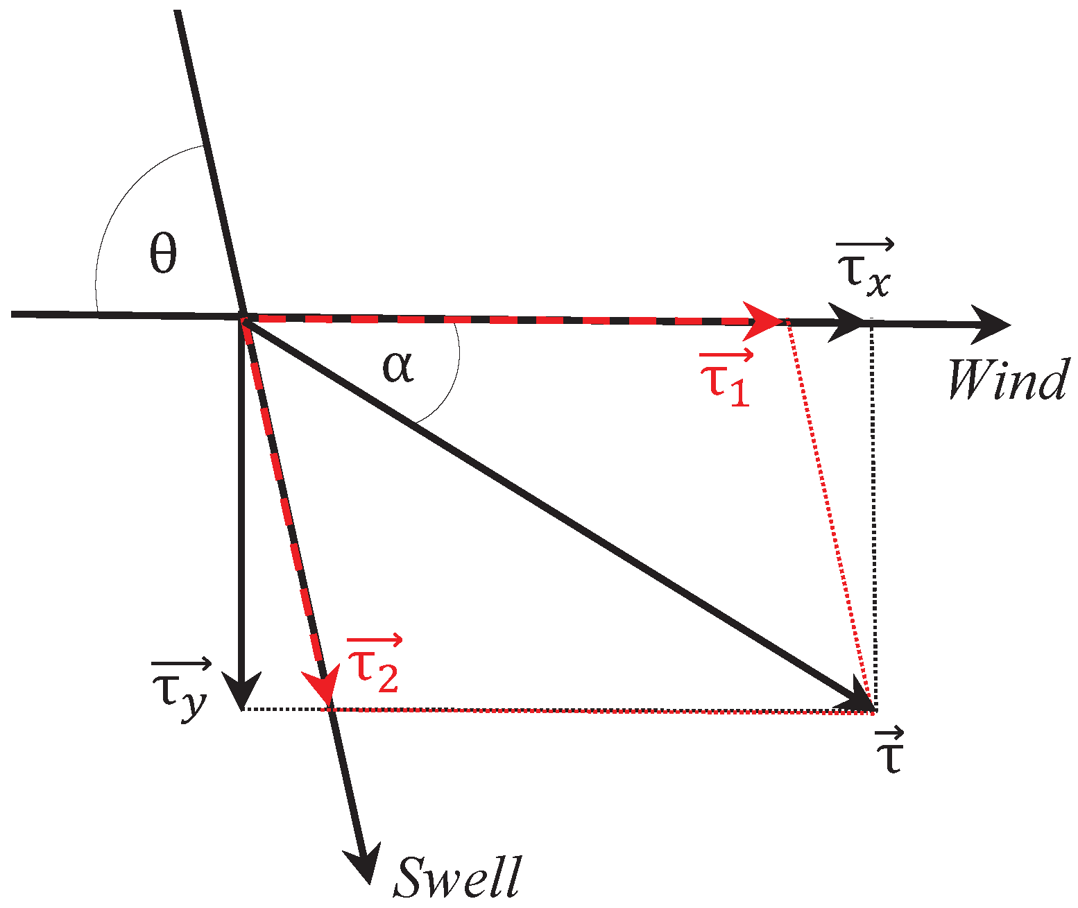
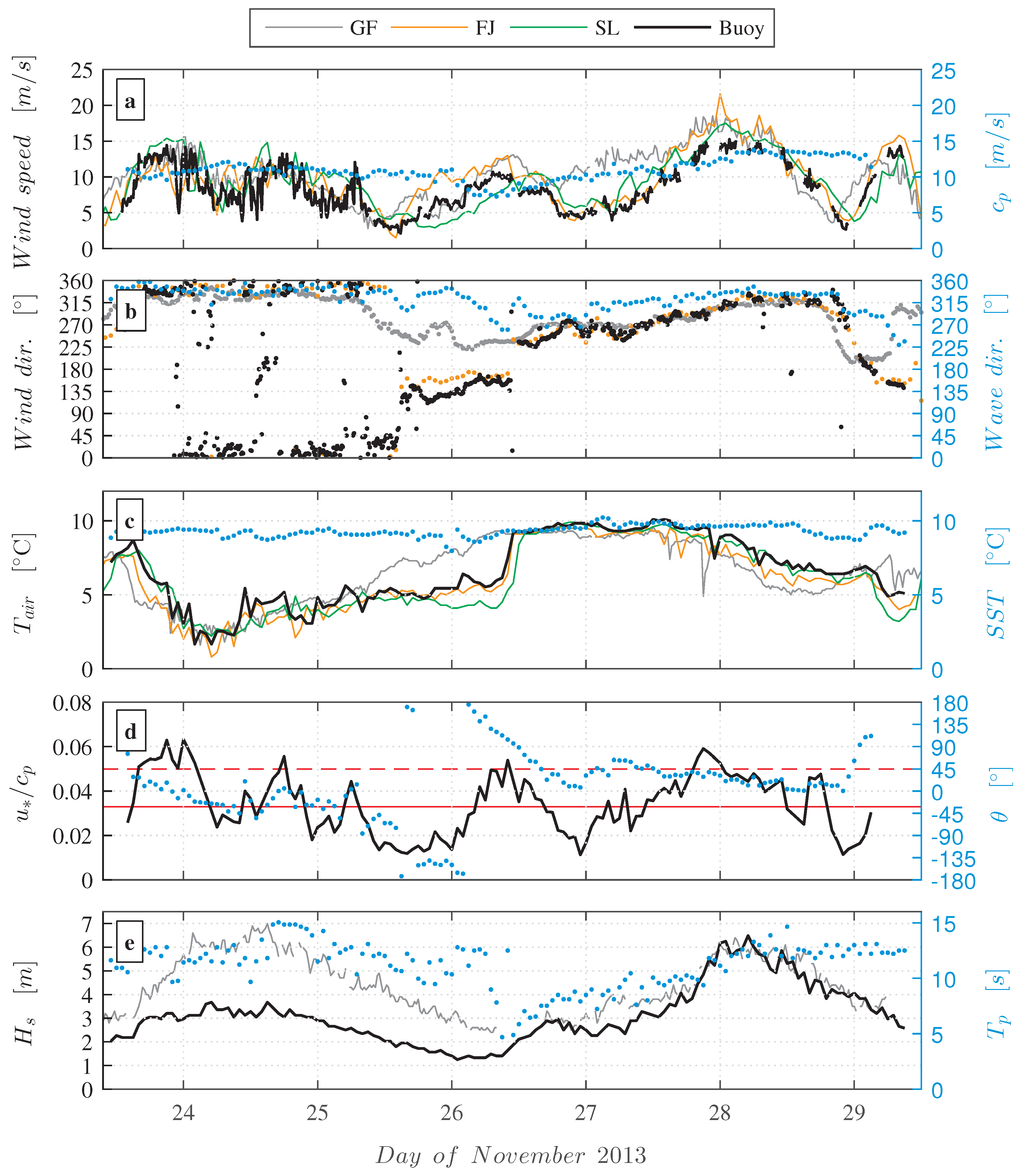
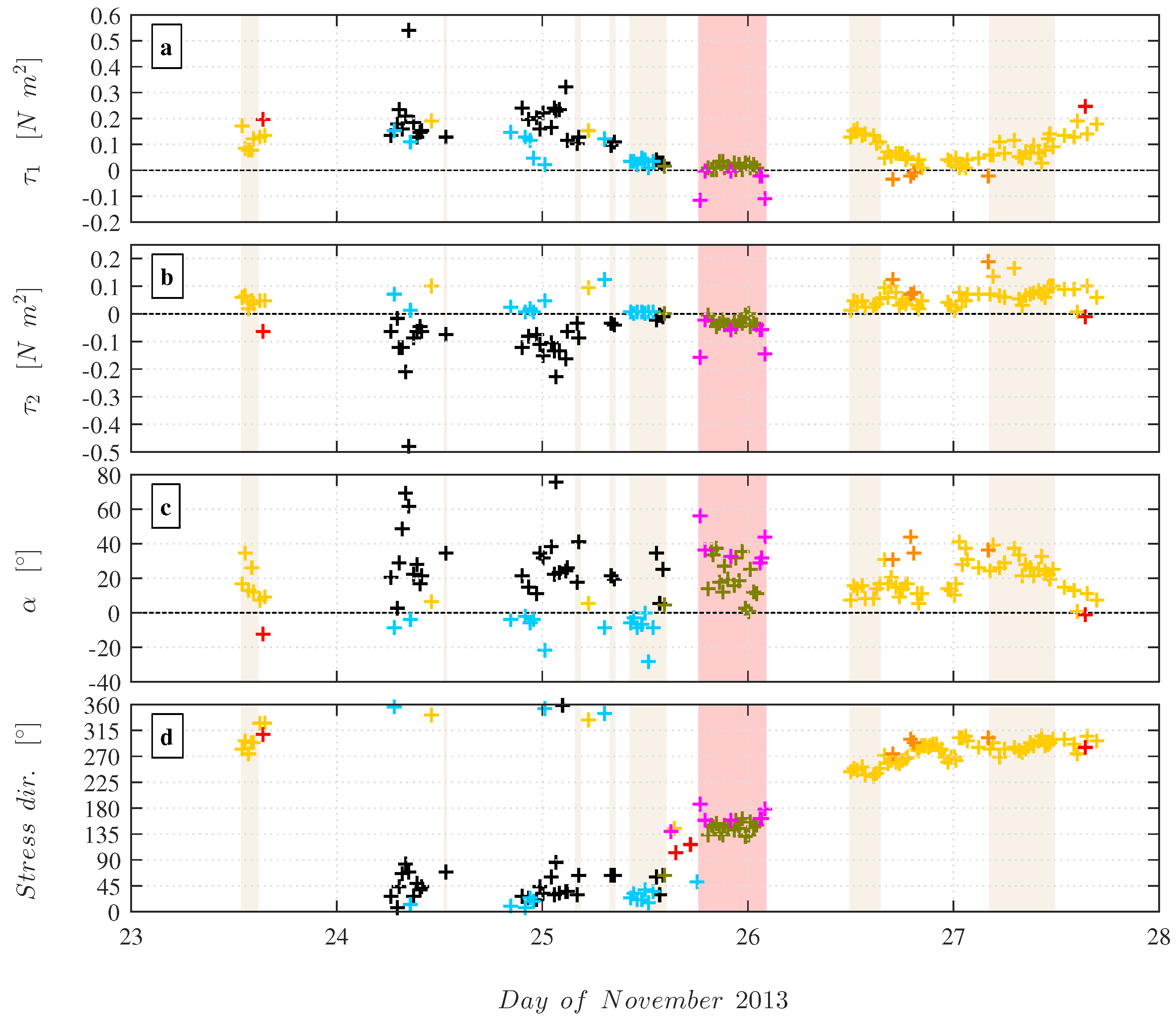
Figure 4 shows the time series of the wind speed and wave phase speed, the wind and wave direction and the along-wind and cross-wind wind stress measured in the orthogonal coordinate system. The color of the data points corresponds to seven observed combinations of the wind stress components ${\mathbf{\tau }}_1$ and ${\mathbf{\tau }}_2$, which are presented in Section 4.2. Time periods associated with cross-swell and counter-swell situations are indicated by the light grey and dark grey shading, respectively.

As expected from the rotation of the recorded wind vector into the streamwise wind, the along-wind stress (${\tau }_x$) was found to be positive for all data runs. Cross-wind stresses (${\tau }_y$) were positive (negative) when the stress off-wind angle $\alpha$ was located to the right (left) of the horizontal wind vector. The majority of the data runs recorded after 26 November were associated with a positive cross-wind stress. The magnitude of the cross-wind stress was found to be generally smaller than the along-wind stress, resulting from the rotation of the wind vector into the streamwise wind. However, the stress magnitude of both ${\tau }_x$ and ${\tau }_y$ was comparable and close to zero for data runs that are associated with cross-swell and counter-swell cases on 25 November and with wind-following swell cases before midnight on 26 November.

Figure 5 shows the magnitude of the corresponding wind stress components, ${\tau }_1$ and ${\tau }_2$, the off-wind angle $\alpha$ and the stress direction. Positive values of ${\tau }_1$ were found for the majority of the data runs. This is regularly observed when winds blow over slower propagating short locally wind-generated waves, which extracts momentum from the wind and leads to further formation and growth of the wind-generated waves [20,24]. Negative values of ${\tau }_1$, both during the counter-swell period on 25 November and also for some of the wind-following swell cases on 26 November, are associated with situations in which the wind speed decreases quickly so that the locally wind-generated waves temporarily travel faster than the wind [20]. Based on the possible combinations of the wind stress direction relative to the wind and swell wave directions, the stress component aligned with the swell wave direction (${\tau }_2$) can acquire differed signs. The stress component ${\tau }_2$ is positive when both the off-wind angle $\alpha$ and the relative angle $\theta$ between the wind and the swell waves have the same sign, and $cos\theta >0$. If the two angles have opposite signs and $cos\theta <0$, ${\tau }_2$ becomes negative. The stress component ${\tau }_2$ is always negative for counter-swell cases in which the swell waves are dragging the wind. This different directions of ${\mathbf{\tau }}_2$ are illustrated in Figure 6 (Section 4.2). Similar to the behavior of the wind stress components in the orthogonal coordinate frame, ${\tau }_1$ and ${\tau }_2$ reached values close to zero on 25 November and before midnight on 26 November. Corresponding estimates of the off-wind angle $\alpha$ between the wind and the stress vector were found to exhibit a large scatter. This is commonly observed in open ocean conditions when the wind is blowing over a swell dominated sea. Based on the sign of the off-wind angle, the stress direction is orientated to either the right or left of the wind direction.

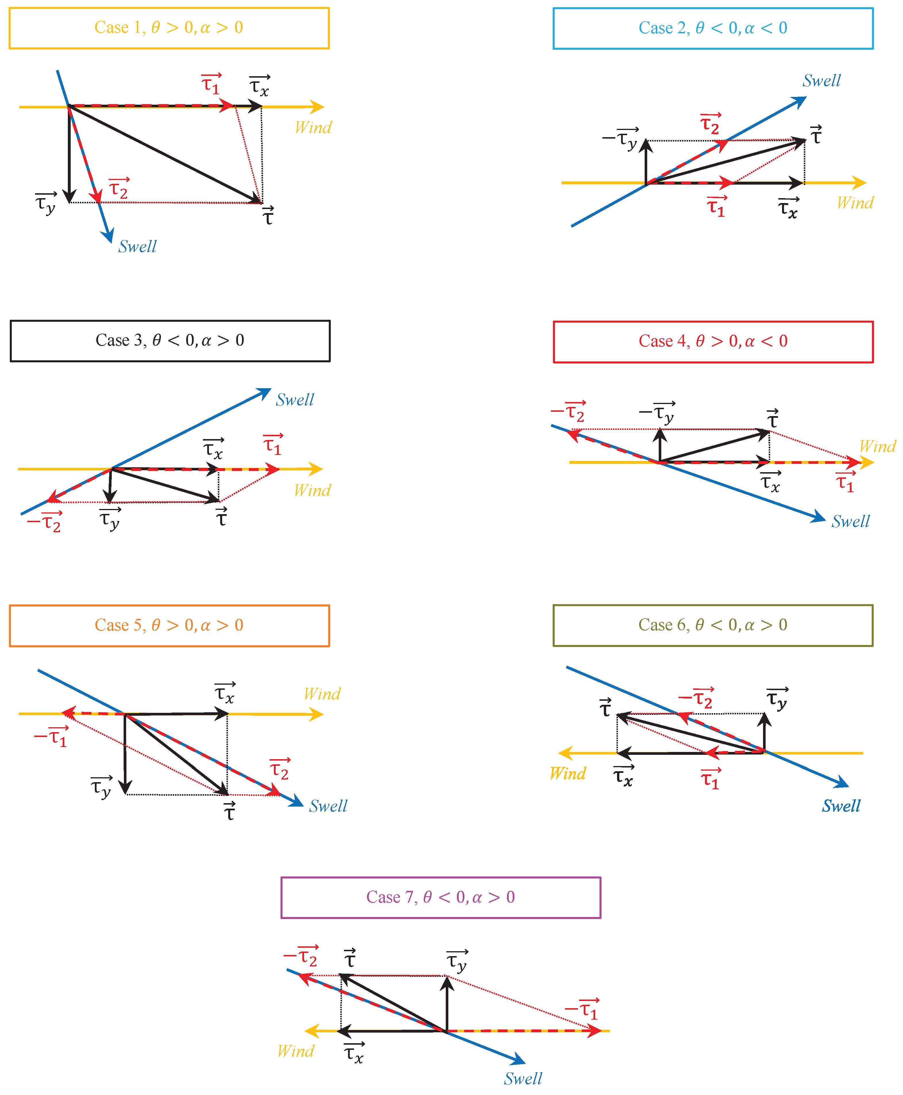
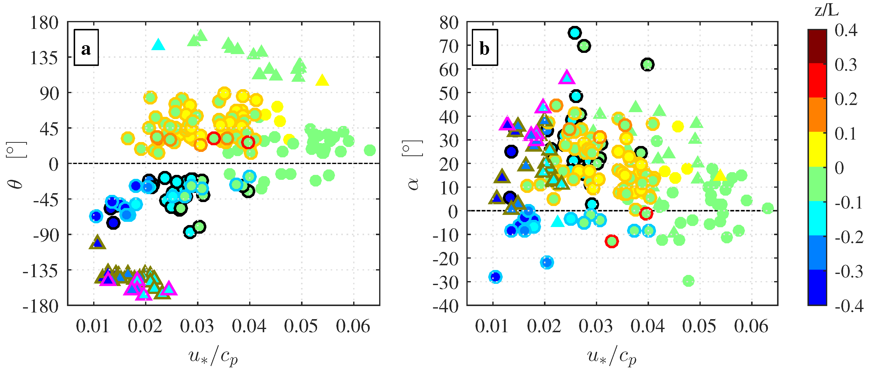
4.2. Schematic Representation of the Observed Stress Vector Components

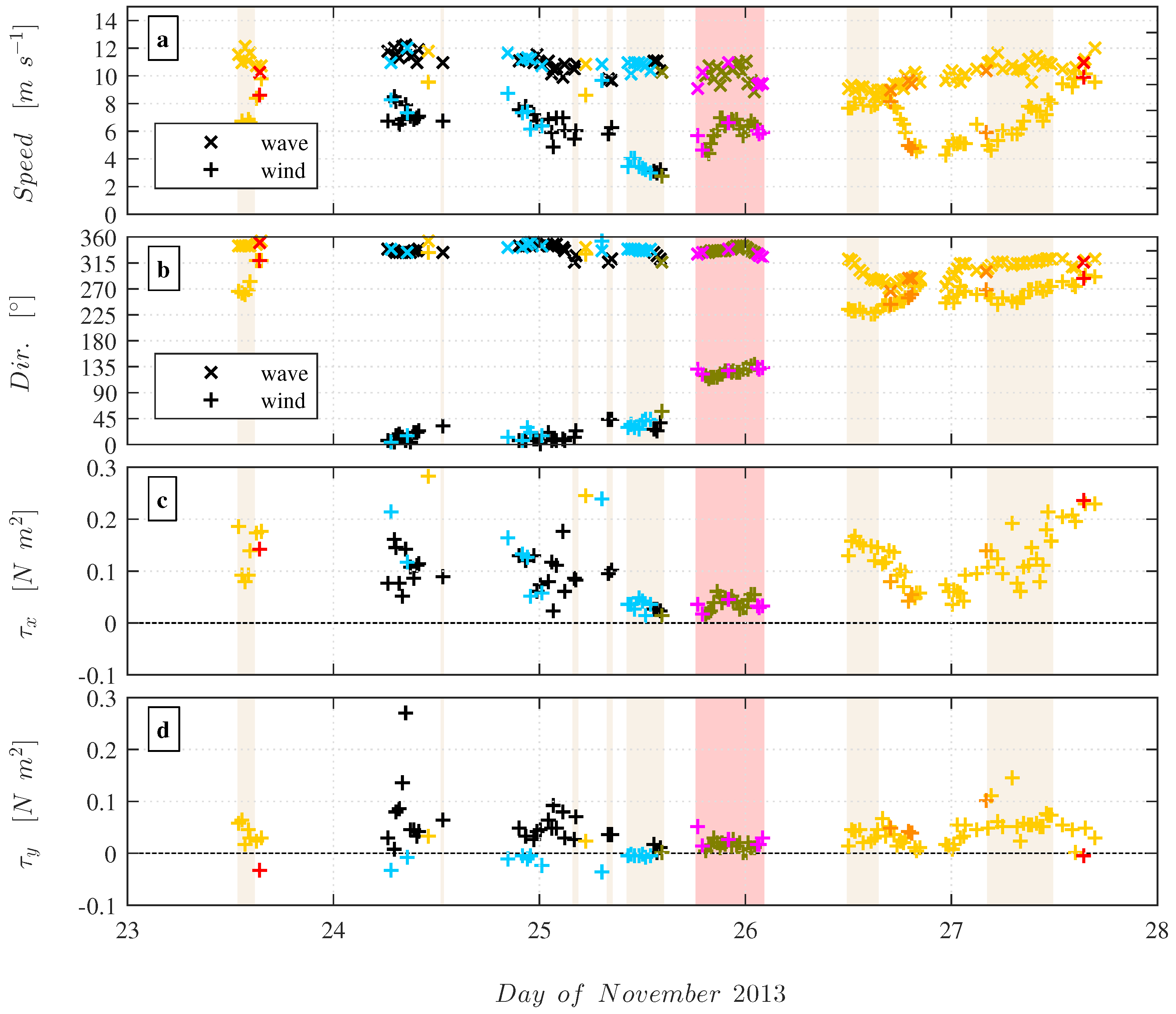
Based on the signs of the relative angle $\theta$ and the off-wind angle $\alpha$, we identified seven idealized combinations of the stress vector direction relative to the wind and swell direction within our dataset. Figure 6 shows a schematic representation of each combination, along with its corresponding stress vector components. For the remainder of this paper, we refer to the identified combinations as “cases”, as shown by different marker edge colors in Figure 4, Figure 5, Figure 6, Figure 7, Figure 8 and Figure 9. Cases 1–5 are associated with wind-following and cross-swell, where $cos\theta >0$.

The stress vector arrangement of Case 1 is typical for situations with moderate to strong winds [20], in which $\theta >0$ and $\alpha >0$. Both ${\mathbf{\tau }}_x$ and ${\mathbf{\tau }}_y$ are positive and the resulting stress vector is situated in the acute angle created by the wind and swell propagation direction, to the right of the wind vector. Consequently, the corresponding stress vector components ${\mathbf{\tau }}_1$ and ${\mathbf{\tau }}_2$ can only be positive. This case was observed at the beginning and from the second half of the deployment period (data runs shown in yellow). The inverted situation, Case 2, occurs when $\theta <0$ and $\alpha <0$. In this case, the cross-wind stress ${\mathbf{\tau }}_y$ is negative while ${\mathbf{\tau }}_1$ and ${\mathbf{\tau }}_2$ remain positive. This situation was observed during 24–26 November (data runs shown in blue).

The stress vector arrangement in Case 3 is typically observed when weak to moderate winds blow over strong swell that travels approximately into the wind direction and faster than the wind [20]. This case is associated with $\theta <0$ and $\alpha >0$, and the stress vector is situated to the right of the wind vector in an obtuse angle created by the wind direction and the direction opposite to the direction of the swell waves. ${\mathbf{\tau }}_x$, ${\mathbf{\tau }}_y$ and ${\mathbf{\tau }}_1$ are positive, while ${\mathbf{\tau }}_2$ is negative and pointing in the direction opposite to the swell propagation direction. This case occurred during 24–25 November (data runs in black). Similar to this case is the inverted situation, Case 4, in which $\theta >0$ and $\alpha <0$. Here, ${\mathbf{\tau }}_x$ and ${\mathbf{\tau }}_1$ are positive while ${\mathbf{\tau }}_y$ and ${\mathbf{\tau }}_2$ are negative and the resulting wind stress vector is situated to the left of the wind vector in an obtuse angle created by the wind direction and the direction opposite to the swell propagation. This case was sporadically observed throughout the deployment period (data runs shown in red).

Case 5 is associated with a decaying wind regime where the locally wind-generated waves travel faster than the wind and thereby exert a drag on the lower meters of atmospheric surface layer. The wind conditions for Case 5 require that the wind is not only strong enough so that ${\mathbf{\tau }}_2>0$, but also weak enough to satisfy ${\mathbf{\tau }}_1<0$ [20]. This case has similarities with Case 1 and is characterized by $\theta >0$ and $\alpha >0$, but the wind stress vector is situated in an obtuse angle created by the swell propagation direction and the opposite wind direction. Within the analyzed dataset, we identified four data runs that fall into this category (data runs shown in orange). Case 6 is associated with a counter-swell situations where $\theta <0$ and $\alpha >0$, with ${\mathbf{\tau }}_x$, ${\mathbf{\tau }}_y$ and ${\mathbf{\tau }}_1$ being positive. The stress vector is situated in the acute angle between the wind direction and the direction opposite to the swell propagation direction, and ${\mathbf{\tau }}_2$ is negative due to wave drag which extracts energy from the atmospheric surface layer [20]. Case 7 is associated with a decaying wind regime where short wind-generated waves travel faster than the wind, i.e., ${\mathbf{\tau }}_1$ and ${\mathbf{\tau }}_2$ are negative. The net stress vector is therefore situated in the obtuse angle between the direction opposite to the swell propagation and the direction opposite to the wind direction. Cases 6 and 7 were both observed on 25 November (data runs in olive and magenta, respectively). Among our seven cases, Cases 1–4 and Case 6 are typically observed during swell conditions and were previously reported by Geernaert et al. [3], Rieder et al. [4], Rieder and Smith [5], Grachev and Fairall [6] and Grachev et al. [20].

4.3. Stress Direction and Stress Magnitude

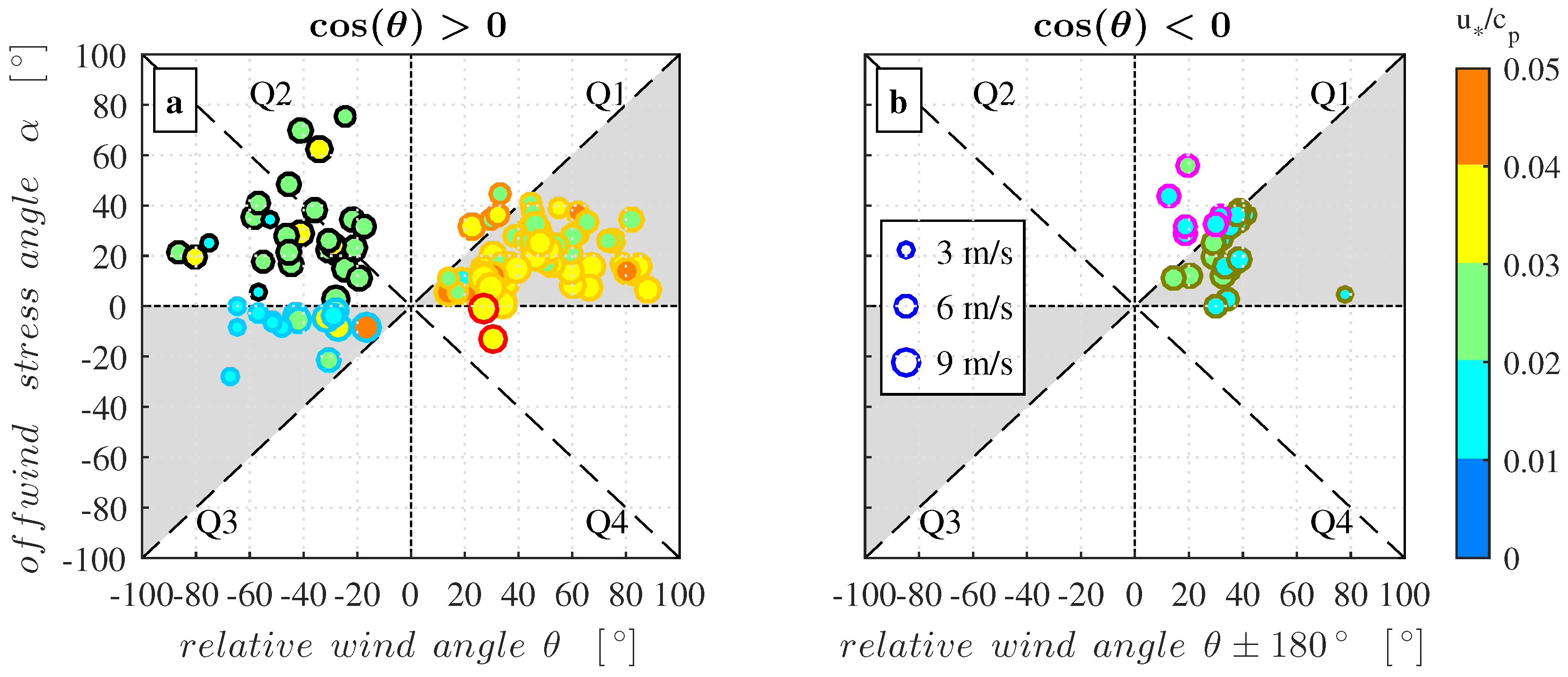
To visualize the direction of the stress vector relative to the wind and swell direction, the off-wind angle $\alpha$ between the stress vector and the wind vector is plotted against the relative angle $\theta$ between the wind and the swell direction in Figure 7. The marker color indicates the wave age, while the marker edge color follows the coding for the different cases given in Figure 6. In general, data points that are aligned with the abscissa, i.e., $\alpha =0$, correspond to runs where the stress angle is aligned with the wind direction. Data points that are located along the dashed diagonal line in Quadrant Q1 and Quadrant Q3 are associated with a wind stress vector that points in the swell propagation direction.

The different cases presented in Figure 6 are distributed as follows: (i) data points situated within the shaded areas in Quadrants Q1 and Q3 of Figure 7a correspond to Cases 1 and 2; (ii) data points situated in Quadrants Q3 and Q4 of Figure 7a correspond to Cases 3 and 4, respectively, while data points outside the shaded area in Quadrant Q1 correspond to Case 5; and (iii) the data points situated in the shaded area of Figure 7b correspond to Case 6, while those points outside this area belong to Case 7. Notably, the majority of the data runs are associated with a wind stress vector that is deviating from the mean wind direction. We found that 46% of the data runs for which $cos\theta >0$ and 54% of the cases for which $cos\theta <0$ have an off-wind angle that is larger than 20°. Moreover, the data exhibit a dependency on both the inverse wave age parameter and on the wind speed. For example, data points for Cases 1 and 5 (Figure 7a, Quadrant Q1), associated with mixed seas and strong winds ($u_{*}/c_p>0.03$, $\overline{U}=$ 7–10 m s⁻¹), have off-wind angles below 20°, while larger off-wind angles are found for data runs associated with a swell dominated sea state and moderate winds ($u_{*}/c_p\le 0.03$, $\overline{U}=$ 4–7 m s⁻¹). Furthermore, most of the data runs associated with Cases 3, 6 and 7 clearly have off-wind angles larger than 20°. Many of the counter-swell runs appear to be closely aligned with the opposite swell direction.

The size of the off-wind angle $\alpha$ is directly related to the magnitude of the stress vector components. A comparison between the wind stress aligned with the wind (${\tau }_1$) and the swell waves direction (${\tau }_2$) is shown in Figure 8. The majority (77%) of the data runs associated with wind-following and cross-swell conditions ($cos\theta >0$) are located within the shaded area in the upper two quadrants of Figure 8a. These data are typically observed for situations where $|{\tau }_1|>|{\tau }_2|$, belonging to Cases 1 and 2 in Quadrant Q1, and to Cases 3 and 4 in Quadrant Q2. Note that the seemingly elongated behavior of the data points in Quadrant Q2 is a result of self-correlation in the solutions of Equation (4). As stated by Grachev et al. [20], this self-correlation can affect the relative positions of the data points within this quadrant but it cannot change the signs of ${\tau }_1$ and ${\tau }_2$. Data runs with stress vector component $|{\tau }_2|>|{\tau }_1|$ are located in the white area of Quadrants Q1 (${\tau }_1>0$, Case 1) and Q4 (${\tau }_1<0$, Case 5). These data account for approximately 23% of the presented data for which $cos\theta >0$, whereof approximately 80% (18% of the presented data for which $cos\theta >0$) have a stress vector that is situated within ±20° of the swell direction. For counter-swell cases (Figure 8b), data associated with the typically observed Case 6 are located in Quadrant Q2, while data belonging to Case 7 are located in Quadrant Q3. We observed that 66% of the counter-swell runs were associated with a stress vector for which $|{\tau }_2|>|{\tau }_1|$ (white area of Quadrants Q2 and Q3). The stress vector was situated within ±20° to the opposite swell propagation direction in 58% of the counter-swell runs.

A dependency on both inverse wave age and wind speed is apparent in Figure 8a. The data are mainly distributed in diagonal bands with an inverse wave age parameter that is increasing with increasing wind speed and wind stress. For wind-following and cross-swell data runs associated with $cos\theta >0$, the lowest values of ${\tau }_1$ and ${\tau }_2$ are associated with strong swell, i.e., $u_{*}/c_p\le 0.02$, and wind speeds below 5 m s⁻¹ (cyan data points). The highest stress estimates are found for wind speeds exceeding 8 m s⁻¹ over a sea mixed with both swell and locally wind-generated waves (orange data points). Unexpectedly, we found that 12 of the 20 data runs which have a stress vector aligned within ±20° of the swell direction were recorded in wind speeds of about 5 m s${}^{-1}$. The remaining eight data runs were recorded in wind speeds up to 8 m s⁻¹. If an interaction between the swell waves and the atmospheric surface layer would affect the wind stress direction, we would have expected that a stress vector alignment towards the swell propagation direction would occur for wind speeds much lower than 5 m s⁻¹.

In counter-swell conditions, the wind is blowing against the waves which increases the surface drag [27,45]. Consequently, the wind stress estimates are expected to be higher than that of the wind-following swell conditions. Nonetheless, our stress estimates recorded during the counter-swell period (Figure 8b) were found to be unexpectedly low. These data runs were recorded during strong swell and wind speeds ranging 4–7 m s⁻¹. The low wind stress values recorded during the counter-swell period would suggest that the atmospheric surface layer at the measurement height was decoupled from the sea surface, so that wind stress was not influenced by the waves. This hypothesis will be further discussed in Section 4.6.

To provide a reference for the stress estimates presented in this study, data reported in Grachev et al. [20] (their Figures 11–13) are also shown in Figure 8. These data consist of three RP FLIP datasets collected by NOAA/ETL and WHOI during the San Clemente Ocean Probing Experiment (SCOPE) in 1993, the Marine Boundary Layer II (MBL II) experiment in 1995 and the Coastal Ocean Probing Experiment (COPE) in 1995 (cf. Grachev and Fairall [6], Grachev et al. [20]). Although the Marstein data were recorded in a coastal area and only 1.2 km from shore, the stress estimates associated with $cos\theta >0$ exhibit a good resemblance with the three RP FLIP datasets that were collected 15 km (SCOPE), 50 km (MBL II) and 20 km (COPE) off the US west coast. For wind-following and cross-swell cases (Figure 8a), the magnitude of the Marstein and RP FLIP wind stress components in Quadrants Q1 and Q4 are comparable, and both datasets consist of cases where ${\tau }_2>{\tau }_1$. Marstein data in Quadrant Q2 were found to be slightly shifted upward compared to the RP FLIP datasets, conceivable due to higher values of ${\tau }_1$ or due to the self-correlation in the solution of Equation (4). For counter-swell cases (Figure 8b), the wind stress magnitudes of the Marstein data are generally comparable to the RP FLIP data runs. Nonetheless, the majority of the counter-swell cases in the Marstein dataset are associated with a wind stress vector that is situated within ±20° to the opposite swell propagation direction, i.e., $|{\tau }_2|>|{\tau }_1|$. In contrast, the counter-swell cases of the three RP FLIP data are clearly associated with a wind stress vector that is more closely aligned with the wind direction vector, i.e., $|{\tau }_1|>|{\tau }_2|$; data located within the shaded area of the Quadrant Q2. Note that the RP FLIP data runs in Quadrant Q1, i.e., ${\tau }_2>0$, correspond to “forbidden” cases as a result of measurement inaccuracies [20].

4.4. Stress Direction and Stability

The relative angle $\theta$ between the wind and the swell is shown as a function of inverse wave age and the stability parameter $z/L$ in Figure 9a. To show the decreasing range of $\theta$ with increasing inverse wave age parameter, and thus increasing wind speed, this figure also includes data runs associated with a complex wind sea, i.e., short locally wind-generated waves are superimposed on top of longer swell waves such that $u_{*}/c_p>0.041$. These data runs are shown without marker edge color and were otherwise excluded from the data analysis. From the data runs included in the analysis, approximately 70% of the wind-following and cross-swell cases for which $cos\theta >0$ were recorded during near-neutral stratifications, i.e., $-0.1<z/L<0.1$ (green and yellow circles with marker edge color). Unstable stratifications ($z/L<-0.1$) occurred only during periods with strong swell ($u_{*}/c_p<0.03$), and include all analyzed counter-swell cases. Interestingly, unstable stratification is almost exclusively associated with negative values of $\theta$. Moreover, it appears that $\theta$ has a relationship with $u_{*}/c_p$ for wind-following and cross-swell cases during unstable stratification, where the relative angle between the wind and the swell wave direction increases with decreasing inverse wave age (cyan and blue circles).

Figure 9b shows the off-wind angle ($\alpha$) as function of the inverse wave age parameter and the stability parameter. Similar to the angle $\theta$, the off-wind angle exhibit a wide range over wave ages related to swell dominated and mixed seas ($u_{*}/c_p<0.041$). The range of $\alpha$ decreases with increasing inverse wave age parameter and wind speed, as reported by, e.g., Drennan et al. [45] and Li et al. [38]. We notice that approximately 87% of the data runs used in our analysis (markers with edge color) have positive off-wind angles. In contrast to the relative angle $\theta$ between the wind and swell direction, both positive and negative off-wind angles are associated with unstable stratification. No clear dependency between $\alpha$ and $z/L$ could be identified in the present dataset. Nonetheless, all data runs belonging to Cases 2 and 4 (data points with blue and red edge colors, respectively) are associated with values of $z/L<0$ and the off-wind angles range between $-10$ and 0°. Data runs recorded over a complex wind sea ($u_{*}/c_p>0.041$) are also associated with $z/L<0$. It remains ambiguous if negative values of $\theta$ and $\alpha$ at the buoy’s deployment site generally are associated with a negative stability parameter (either unstable or near-neutral stratification), or if these observations are a result of the limited number of performed measurements. It also remains unclear why data runs belonging to Cases 2 and 4 only have small negative off-wind angles. These data runs are related to moderate winds (3–5 m s⁻¹) that blow over a strong cross-swell during an unstable stratification ($u_{*}/c_p<0.02$, cyan and blue markers), and moderate to strong winds of 6–9 m s⁻¹ that blow over a wind-following swell in near-neutral conditions (green markers with edge color). The small off-wind angles suggest that the stress vector is roughly aligned with the wind direction and that, contrary to the remaining data, the swell waves have little or no influence on the wind stress direction. For example, data runs with both $\alpha <0$ and $u_{*}/c_p<0.02$ (cyan and blue markers) were found to have a lower wave steepness ($ws=$ 0.02–0.03) than the remaining cross-swell and wind-following swell cases ($ws=$ 0.03–0.06) (not shown). We speculate that the small off-wind angles associated with Cases 2 and Case 4 could result from a combination of an unstable stratification and a low wave steepness. The low wave steepness might reduce the amount of swell wave-induced dynamic pressure perturbations at the sea surface, which contributes to the form stress (cf. Högström et al. [46]). Simultaneously, the upward transport of the pressure perturbations (due to vertical displacement of the air by the swell waves) into the lower meters of the atmospheric surface layer is effectively reduced by the unstable stratification. Support for this speculation can be found in Figure 8a. Stress estimates for Case 2 associated with $u_{*}/c_p<0.02$ (cyan data points) are located close to the ordinate axis, i.e., ${\tau }_2\approx 0$. This indicates that the wind stress component ${\tau }_2$, which is aligned with the swell wave direction, is negligible for these data runs. The wind stress would thus mainly be supported by the component ${\tau }_1$, and this would explain the observed small off-wind angles for Case 2. Moreover, the results in Section 4.6 indicate that these data runs might be associated with a land-footprint and the formation of an internal boundary layer. It is reasonable to assume that the surface roughness of the land is higher than the surface roughness of the swell waves. A higher surface roughness will increase the shear stress and thus contribute to an increase of ${\tau }_1$ (Equation (7)). Therefore, a land-footprint might also contribute to keep the wind stress vector aligned with the wind direction.

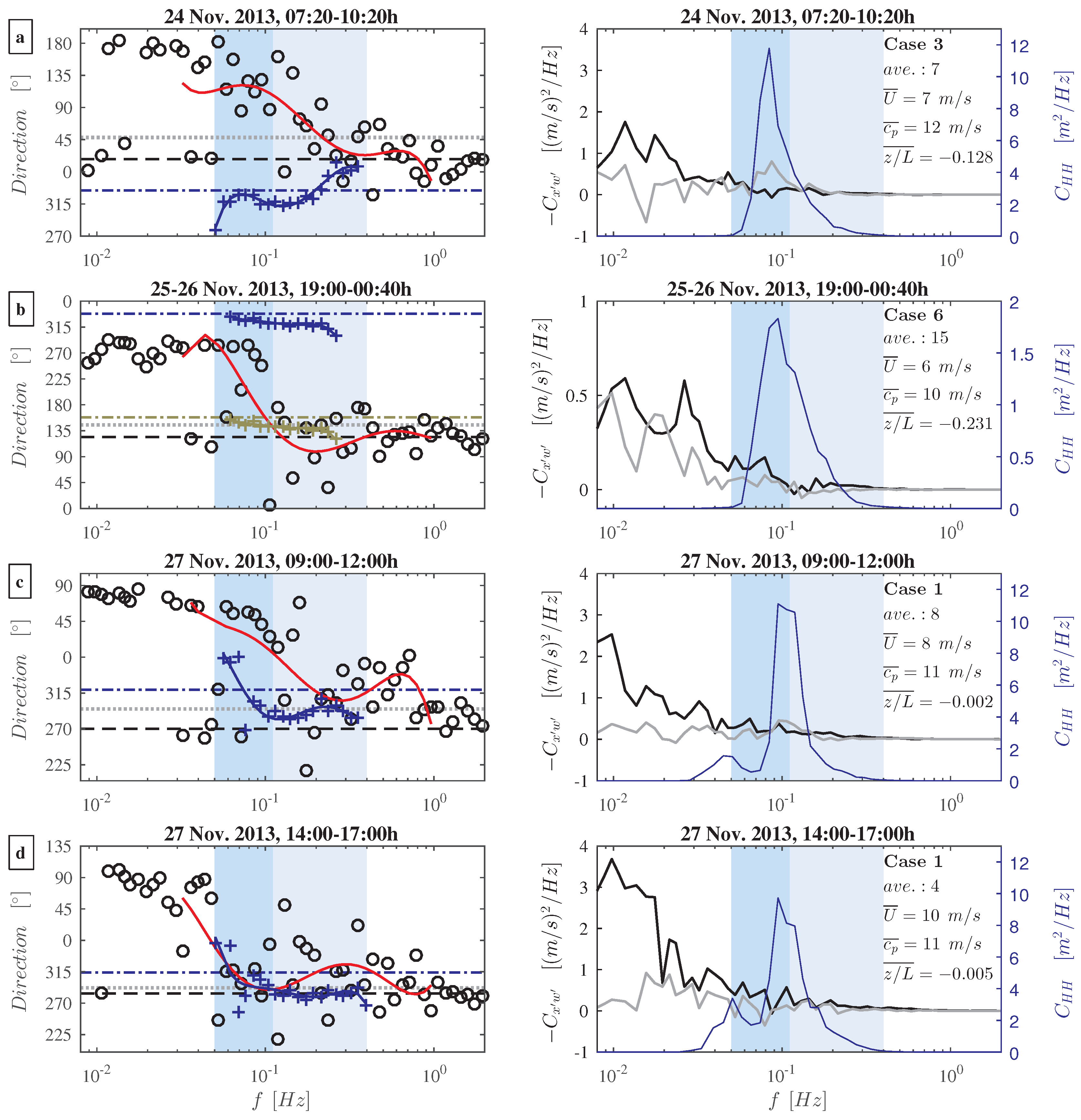
4.5. Spectral Description of the Wind Stress and Wave Direction

The deviation of the stress vector from the wind direction can be further examined from the spectral description of the wind stress direction. For this, we followed the approach of Rieder et al. [4] and computed the off-wind angle between the stress vector and the wind vector as a function of frequency:

$$A\left(f\right)={tan}^{-1}(C_{v^{\prime }{w}^{\prime }}/C_{u^{\prime }{w}^{\prime }}),$$

(8)

where $C_{u^{\prime }{w}^{\prime }}$ and $C_{v^{\prime }{w}^{\prime }}$ are the real parts of the vertical momentum flux cospectra in the along-wind and cross-wind direction, respectively. The resulting off-wind angles were then binned by logarithmic averaging over uniformly spaced “log10” frequency bands. The corresponding net-stress directions were obtained as a function of frequency by adding the mean wind direction to the binned off-wind angles of $A\left(f\right)$. The net-stress direction can be compared with the directional wave spectra to highlight interdependencies between the wind stress and the waves at different frequencies.

Data for the peak and mean wave directions were recorded by the Wavescan buoy. However, the directional wave spectra that were computed by the buoy’s internal data processing unit were not stored. To obtain estimates of the wave directions at different frequencies, we used the IMU accelerometer data and applied a modified PUV-approach, as described by Flügge et al. [35]. It is emphasized that the computed directional wave spectra are only estimates and can, on average, differ from the “true” wave directions by up to 20° [35]. Nonetheless, peak and mean wave directions computed by the modified PUV-approach were found to be in relatively good agreement with the corresponding wave direction data from the Wavescan buoy (not shown). We are therefore confident that the wave direction spectra computed by the modified PUV-approach are reliable.

To minimize errors in the wind stress directions computed with Equation (8), stress direction estimates of successive data runs were averaged together. This requires that the relative angle $\theta$ between the wind and the swell direction exhibits only small variations between successive data runs [4]. Within the present dataset, we identified four time periods in which the variation of $\theta$ between successive data runs is smaller than 8°. Estimates of the wind stress and the wave direction as function of frequency for these four time periods are shown in the left column of Figure 10. To better visualize the turning of the wind stress and wave directions, a fifth-order least-square-fit polynomial is drawn through both the stress and wave direction data (cf. Rieder et al. [4]) over the frequency range of 0.03–1 Hz, which corresponds to wave periods between 1 and 30 s. We found that a fifth-order fit is most suitable to display the change of the wind stress direction in our data. Note that three data points in Figure 10b and four data points in Figure 10c, corresponding to frequencies below $f\le$ 0.06 Hz and directions below 180° and 320°, respectively, were excluded from the calculation of the fifth-order polynomial fit in order to remove artifacts resulting from the fitting procedure. The right column of Figure 10 shows the corresponding heave variance spectra and the along-wind and cross-wind cospectra for each time period. Figure 10 also gives the numbers of averaged data runs and the corresponding mean values of the wind speed recorded at the sonic anemometer, the wave phase speed and the stability parameter at the measurement height.

Figure 10a shows estimates of the wind stress and wave directions for a 3 h period on 24 November. This time period consists of data runs belonging to Case 3 (Figure 6), which had a mean net-wind stress directed 30° to the right of the mean wind direction. The wave field contained waves with periods between 3 and 20 s and the average relative angle between the wind and the waves, $\overline{\theta }$ was −44°, i.e., to the left of the mean wind direction. Short waves with $f\ge 0.25$ Hz and the corresponding wind stress directions were roughly aligned with the mean wind direction. This supports our assumption made in Section 2 that the short waves approximately propagate into the mean wind direction. For $f<$ 0.25 Hz, the wave direction turned counter-clockwise with decreasing frequency ($\theta <0$), while the corresponding estimates of the wind stress direction turned clockwise ($\alpha >0$). Although we only have a limited amount of data, it can be speculated that the turning of the waves and wind stress into opposite directions at frequencies larger than 0.25 Hz might indicate that only short waves with periods lower than 5 s are concurrent with the wind stress in situations associated with Case 3.

Estimates of the wind stress and wave directions for a 5.5 h counter-swell period corresponding to Case 6 are shown in Figure 10b. For convenience, the opposite wave directions and the mean value of the opposite average wave direction are shown in olive green. The net-wind stress was orientated 22° to the right of the mean wind direction, in between the mean wind direction and the direction opposite to the average wave direction. The relative angle between the mean wind and the average wave direction was −145°, while the relative angle between the mean wind and the opposite average wave direction was 35°. Waves with periods between 4 and 16 s were present during the counter-swell period, and the shortest waves at $f\sim 0.25$ Hz were aligned close to the mean wind direction. The wave direction was slightly turning clockwise with decreasing frequency and the longest swell waves at $f=0.06$ Hz were closely aligned with the average wave direction. Estimates of the wind stress direction are scattered around the mean wind direction within the frequency band of the locally wind-generated waves. The fifth-order polynomial fit indicates that the wind stress was orientated to the left of the mean wind direction within most of this frequency band. Within the swell wave frequency band, the wind stress turned clockwise, i.e., to the right of the mean wind direction, with decreasing frequency.

Estimates of the wind stress and wave direction for the typically observed Case 1 are presented in Figure 10c,d, which show estimates for two different 3 h time periods on 27 November. During the first time period (Figure 10c), the wave field contained waves with periods between 3 and 20 s and the average wave direction was 49° to the right of the mean wind direction. The mean net-wind stress direction had an angle of 25° to the right of the mean wind direction and was thus situated between the mean wind and average wave direction (Figure 6, Case 1). Many of the locally generated short wind waves at $f\sim$ 0.1–0.2 and $f\ge 0.3$ Hz appear to have been roughly aligned with the mean wind direction. Waves with frequencies of 0.1–0.2 Hz seem to have a slightly different propagation direction concurrent with the net-wind stress. Nonetheless, the estimated wave directions within this frequency band might be uncertain due to limitations in the modified PUV-approach [35]. Estimates of the wind stress direction are situated between the mean wind and the average wave direction in the frequency range of 0.2–0.35 Hz, which is similar to the observations presented by Rieder et al. [4]. Wind stress directions appears to have been more aligned towards the average wave direction for frequencies of 0.35–0.8 Hz. This might indicate the existence of non-stationary processes at the measurement site, as well as residual noise from incomplete motion correction. The estimates of both the wind stress direction and the wave direction turned clockwise within the swell wave frequency band. The fifth-order polynomial fit suggests that the turning of the wind stress direction started at a slightly higher frequency ($f\sim 0.1$ Hz) than the turning of the wave direction. Consequently, the relative angle $\theta$ between the wind and the swell waves was larger for shorter swell waves and decreased with decreasing frequency for longer swell waves.

During the second period on 27 November (Figure 10d), the average wind speed increased and was close to the phase speed of the waves. The peak wave direction became more aligned with the mean wind direction as $\overline{\theta }$ decreased to 30°. Moreover, the angle between the mean wind and the net-wind stress direction decreased to 8°, and the net-wind stress direction was thus closely aligned with the mean wind direction. In comparison to the first period on 27 November, the direction for most of the locally wind-generated waves became co-directional with the mean wind direction. The corresponding estimates of the wind stress direction in this frequency band were found to be scattered around the mean wind and the average wave direction. The fifth-order polynomial fit suggests that wind stress had a tendency to be directed towards the average wave direction for $f\ge 0.2$ Hz. Within the swell wave frequency band, the estimates of the wind stress and the wave direction were found to be in reasonable agreement.

Common for all four time periods in Figure 10 is a change of the wave direction with decreasing frequency and a corresponding change of the wind stress direction, particularly in the swell wave frequency band. This is illustrated in Figure 10a–c where a clear clockwise turning of the wind stress direction can be seen in this frequency band. Moreover, the fifth-order polynomial fit in Figure 10b–d appear to resemble the turning of the waves, which is similar to the findings in Rieder et al. [4]. This suggests an interdependency between the wind stress and the swell waves, i.e., the direction of the wind stress in at the buoy’s deployment site is influenced by the swell waves despite its vicinity to the coast. Support for this observation can found from by the respective heave variance spectra and the along-wind and cross-wind cospectra in the right column of Figure 10. It is reasonable to assume that any interdependency between the wind stress and the surface gravity waves can only take place within the frequency band of the wave field, i.e., all frequencies covered by the respective heave variance spectra. The along-wind and cross-wind cospectra show that the spectral energy of the wind stress was negligible at frequencies corresponding to the locally wind-generated waves, i.e., $f\ge$ 0.2 Hz in all four time periods. The spectral energy of the wind stress is increasing with decreasing frequency and a pronounced increase in the spectral energy of the wind stress is first visible within the swell wave frequency band. This implies that an interdependency between the wind stress and the wave field must occur in the swell wave frequency band because the wind stress has not sufficient energy at higher frequencies to influence the wind stress. The influence of swell waves on the wind stress direction in the open ocean was previously reported by Geernaert et al. [3], Rieder et al. [4], Rieder and Smith [5], Grachev and Fairall [6] and Grachev et al. [20].

Interestingly, it appears that the clockwise turning of the wind stress and waves direction was out of phase during the first time period on 27 November (Figure 10c). We expected to see a similar behavior in the turning of the wind stress and wave direction, as shown in Figure 10d, due to the almost similar conditions during the two time periods. An explanation for the differences between these two time periods might be related to the increased spectral energy at the peak wave frequency in the cross-wind cospectra seen in Figure 10a (Case 3) and Figure 10c (Case 1). A corresponding increase in spectral energy in the cross-wind cospectra is absent during the second time period of 27 November (Figure 10d). We speculate that the larger angle between the mean wind and the average wave direction in the first time period led to a slightly increased cross-wind stress around the peak wave frequency, which is situated at the transition between the frequency range of the wind-generated and the swell waves (Figure 10c). The air-flow close to the sea surface might have felt the most energetic swell waves (at the peak wave frequency) that were travelling at a cross-wind angle relative to the mean wind direction ($\overline{\theta }=49{}^{\circ }$). The stress direction in Figure 10c suggests that the turning of the wind stress occurred at the peak wave frequency, while the turning of the swell wave direction occurred at slightly lower frequencies. In the second time period of 27 November (Figure 10d), the relative angle between the mean wind direction and the peak wave direction decreased to $\overline{\theta }=30{}^{\circ }$, and the wind stress directions within the swell wave frequency band were situated between the mean wind and the average wave direction. We further hypothesize that the cross-directional forcing of the most energetic swell waves on the air flow might not have been strong enough to influence the wind stress direction at the peak wave frequency. Nonetheless, the wind stress estimates in Figure 10d suggest that the stress direction did undergo a clockwise tuning which occurred at the lowest swell wave frequency, $f\sim 0.05$ Hz. At this frequency, the corresponding heave variance spectra exhibit an additional small spectral peak. We suggest that the longest swell waves, which were propagating at an angle of ∼80° and ∼50° to the mean wind direction and average wave direction, respectively, have contributed to the clockwise tuning of the wind stress direction in the second period of 27 November.

4.6. Case Study-Counter-Swell Period

The comparison between the Marstein dataset and the three datasets collected aboard RP FLIP (Section 4.3, Figure 8) shows that our wind stress estimates are in good agreement with open ocean wind stress measurements, except for the counter-swell period. When winds blow against the waves, the wind stress is expected to be higher than in the wind-following swell conditions [27,45]. Nonetheless, the wind stress recorded at Marstein was found to be unexpectedly low during the counter-swell period. In this section, we attempt to provide an explanation for this seemingly paradoxical observation.

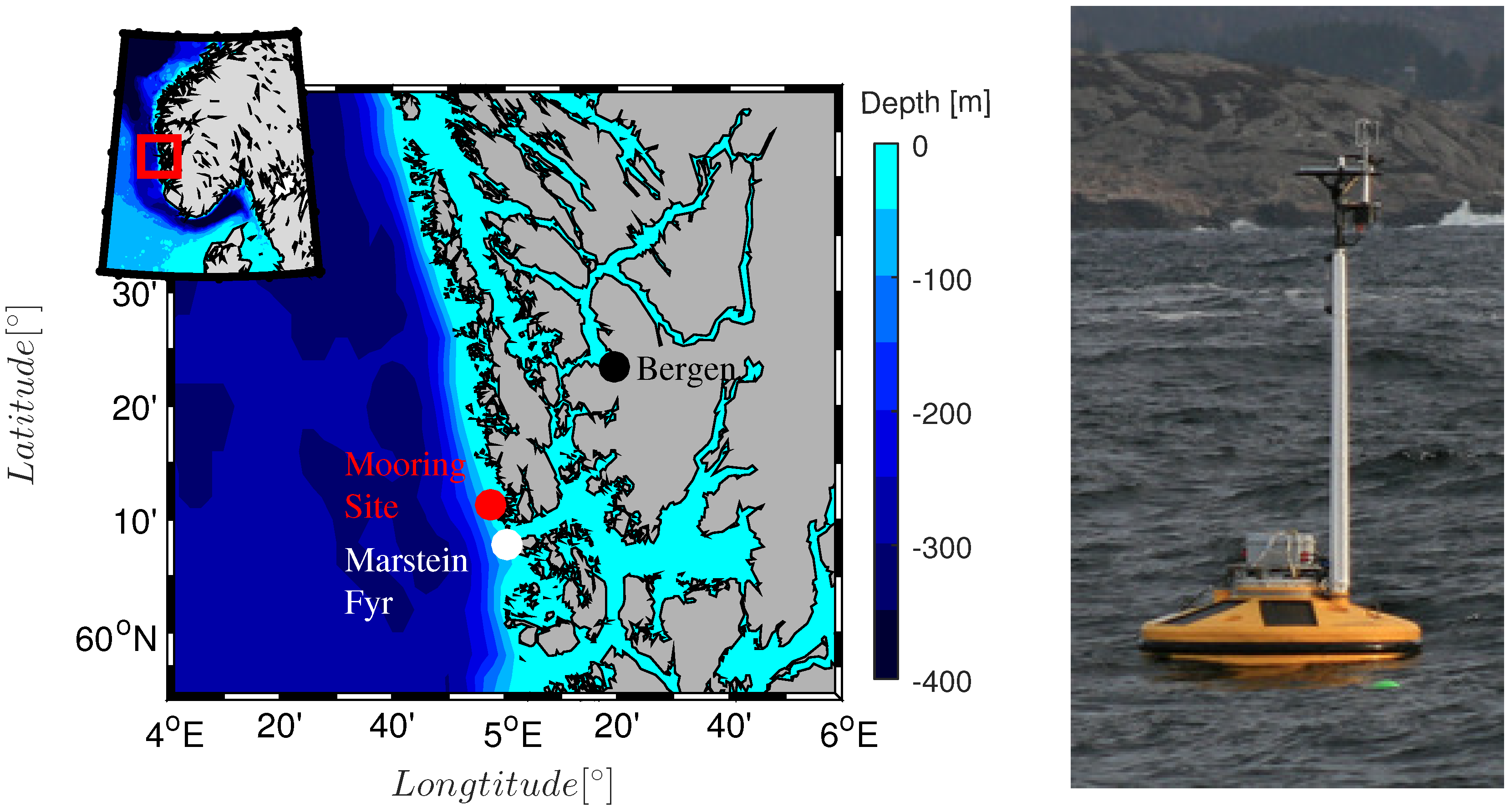
During the first two days of the buoy’s deployment period, the wind was blowing from a northwest to northerly direction (Figure 3b). On the morning of 25 November, the wind direction changed clockwise towards a northeasterly direction (25–45°) for a period of approximately 5 h, before a sudden shift in wind direction towards southeasterly (115–145°) occurred. The southeasterly winds prevailed for a period of 19 h in which the wind slowly turned more southerly, before the occurrence of a new sudden (clockwise) shift towards southwest on 26 November. The two distinct shifts in wind direction are clearly visible in Figure 3b, and were also recorded at the Fedje met-station (orange dots in Figure 3b). Moreover, the second shift in wind direction on 26 November was accompanied by a distinct increase in air temperature, which increased by approximately 4 °C and reached the same value as the sea surface temperature. Interestingly, no sudden shifts in wind direction or air temperature were recorded at the Gullfaks C oil platform in the North Sea. The wind direction at Gullfaks turned gradually counter-clockwise from northwesterly to southwesterly on 25 November, and the air temperature gradually increased by approximately 4 °C between 25 and 26 November (grey dots and line in Figure 3b,c). The sudden changes in wind direction, in combination with the sudden increase in air temperature, suggest that local boundary layer processes were affecting the WaveScan buoy’s deployment site 1.2 km offshore. Figure 3a,b shows that the turning of the wind to a north-easterly direction on 25 November is accompanied by a drop in wind speed from 10 to 5 m s⁻¹. During the 5 h period with north-easterly winds, the wind speed decreased further to approximately 3 m s⁻¹. Note that the sudden change towards a south-westerly wind direction occurred at this wind speed, which was the lowest recorded wind during the deployment period.

We hypothesize that the temperature difference between the land and the sea, in combination with the low wind speed and the unstable atmospheric stratification, led to the onset of a land breeze circulation. Winds blowing towards the sea near the ground would extended the lower part of the land boundary layer further offshore, where the cool air would warm and raise upward. If the wind direction is reversed higher up, the wind would extend the marine atmospheric boundary layer over the coastal areas of the land, where the warmer air would cool and sink downward. The land breeze would thus lead to a mixing between the marine atmospheric boundary layer and the land boundary layer.

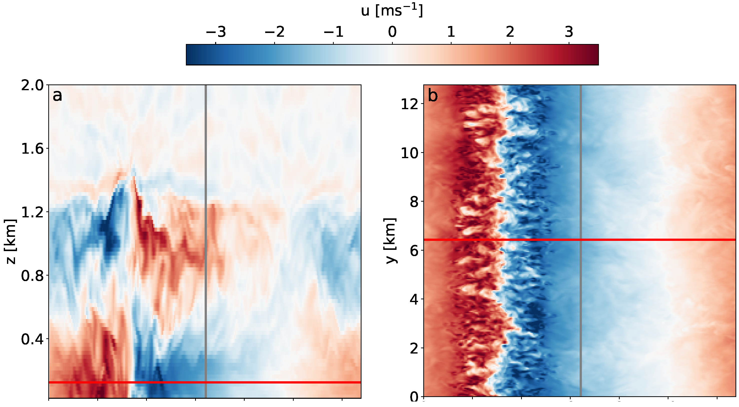
In a first attempt to evaluate the hypothesis that the southeasterly winds during the counter-swell period were associated with a land breeze circulation caused by the temperature gradient between the warmer sea and the colder land, we performed an idealized LES simulation with PALM (Parallelized Large-Eddy Simulation Model) [47]. The simplistic setup consisted of a north–south oriented coastline that separates a surface with a constant temperature of 10 °C to the west (sea) from one with 0 °C to the east (land). The simulation was initialized without background wind and run for 12 h. For more details on the PALM model in general, and the specific setup used for this study, the reader is referred to Appendix A.

Figure 11 presents a snapshot from the LES simulations after 6 h modelling time. It shows the development of a land-breeze circulation with easterly winds of about 300 m depth that reaches nearly 3 km offshore. The highest wind speeds of around 3 m s⁻¹ are found at a distance of 2 km from the coast, very close to the offshore distance of the buoy in our study. How far the mixed boundary layer extends offshore typically depends on the strength of the land breeze, the atmospheric stability and on fetch limitations. The results of our LES simulation indicate that our measurement site 1.2 km offshore is well inside the potential reach of a land breeze circulation, and thus our measurements might have been performed within a mixed boundary layer rather than in a pure marine atmospheric boundary layer during the counter-swell period with prevailing southeasterly winds.

Nonetheless, even within a mixed boundary layer, increased wind stress is expected when the wind is blowing against the waves. Given that the observed wind stress was low during the counter-swell period, we further hypothesize that the mixed boundary layer was decoupled from the undulating sea surface. The mixed boundary layer might have acted as an internal (transition) boundary layer that was situated between the wave boundary layer and the marine or land atmospheric boundary layer higher up. Turbulence generation due to shear stress and wave stress (Section 2), and hence the exchange of momentum from the atmosphere to the ocean, might only have occurred within a shallow wave boundary layer up to 3 m above the sea surface (cf. Cifuentes-Lorenzen et al. [21]), thus leaving the internal boundary layer decoupled from the wave boundary layer.

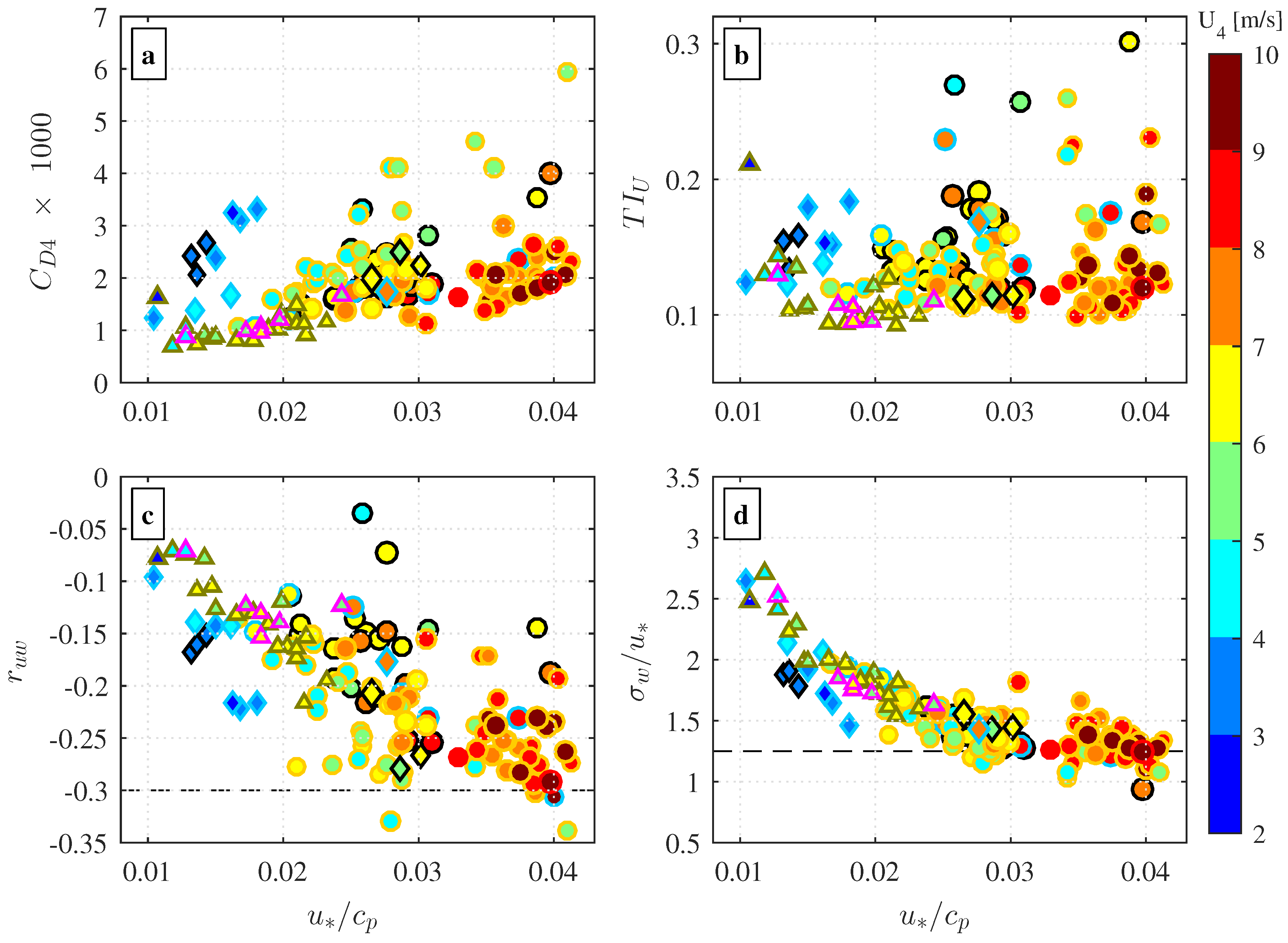
Within a decoupled internal boundary layer, one would expect only low turbulence generation and thus only weak wind stress. An indication for this can be seen in Figure 12, which shows the drag coefficients, the turbulence intensities for the along-wind component, the correlation coefficients between u and w and the normalized vertical velocity standard deviations, computed for the measurement height of 4 m above the sea surface. The drag coefficients in Figure 12a reveal the presence of three wind regimes during the buoy’s deployment period: (1) a regime for winds blowing from open ocean directions and associated with wind-following and cross-swell (shown as circles); (2) a regime for winds blowing over land towards the sea from northeasterly directions and associated with cross-swell (shown as diamonds); and (3) a regime for winds blowing over land towards the sea from southeasterly directions and associated with counter-swell (shown as triangles). The first wind regime (circles) exhibits the typically observed dependency of the drag coefficient on the inverse wave age parameter and wind speed (cf. Edson et al. [25], Smedman et al. [48]). This dependency is expected, as higher winds will increase the sea surface roughness and thus the wind stress. The second regime is characterized by high drag coefficients, especially for wind speeds below 5 m s⁻¹ (cyan and blue diamonds) where the drag coefficients appear to be much higher compared to the other two wind regimes. Moreover, turbulence intensities for wind speeds below 5 m s⁻¹, both for horizontal and vertical velocity components, were found to be equal or higher than the turbulence intensities recorded in the other two wind regimes. Note that the Case 2 data runs with wind speeds below 5 m s⁻¹ (cyan and blue diamonds with blue edge color) are associated with low off-wind angles (Figure 9). We therefore suggest that data runs associated with northeasterly winds had a land-footprint and that the deployment site, in fact, was situated within a mixed boundary layer. This is similar to recent findings presented by Grachev et al. [11]. The third wind regime succeeded the second wind regime and is clearly distinguished from the other two wind regimes by low drag coefficients and low turbulence intensities (triangles). If the boundary layer was fully coupled with the sea surface, we would expect that these data runs have high drag coefficients and turbulence intensities, resulting from enhanced wind drag on waves travelling in the opposite wind direction and from enhanced shear stress due to land-footprints. However, the analyzed data clearly show reduced drag coefficients and turbulence intensities for counter-swell cases. This suggests that shear turbulence generation processes at the measurement height of 4 m were either suppressed or absent, which supports our hypothesis of a decoupling between the undulating sea surface and the atmospheric boundary layer. Although the wind stress estimates recorded during the counter-swell period were small and therefore subject to measurement errors, the data indicate that the wind stress component aligned with the wind direction (${\mathbf{\tau }}_1$) was close to zero for most of the presented counter-swell runs. The corresponding wind stress component aligned with the (opposite) swell direction (${\mathbf{\tau }}_2$) was found to be slightly larger. In the absence of sufficient turbulent shear production, i.e., ${\mathbf{\tau }}_1={\mathbf{\tau }}_{shear}+\widetilde{{\mathbf{\tau }}_1}\approx 0$, the wind stress vector has to align itself towards the opposite swell wave propagation direction, i.e., $\mathbf{\tau }={\mathbf{\tau }}_1+{\mathbf{\tau }}_2\approx {\mathbf{\tau }}_2$. This explains why the wind stress direction for the majority (58%) of the counter-swell cases was situated within ±20° to the opposite swell propagation direction (Figure 7 and Figure 8).

The mechanism behind a decoupling between the sea surface and the atmosphere during counter-swell remains ambiguous. A decoupling between the ocean and the atmosphere would likely occur in wind-following and cross-swell situations with strong background swell and weak winds. Such a situation was reported by Smedman et al. [49,50], where fast travelling swell waves transported momentum from the ocean to the atmosphere, thus counteracting the downward transport of momentum from the atmosphere to the ocean. However, the opposite directions between the wind and the swell waves during counter-swell will always lead to an enhanced wind stress, and thus transport of momentum from the atmosphere to the ocean. Another mechanism could be related to negative values of ${\mathbf{\tau }}_1$, i.e., data runs associated with Case 7. In these situations, the short wind-generated waves travel faster than the wind and transfer momentum to the atmosphere. During periods of decreasing weak winds with low shear turbulence production, the upward transport of momentum from the short waves could counteract the weak downward transport of momentum from the atmosphere to the ocean. However, as the wind generates the short waves, the sea state will adapt itself after a short period of time so that this special situation cannot last long. Therefore, it seems unlikely that air–sea interaction processes could be responsible for a decoupling between the atmosphere and the ocean during counter-swell.

Nonetheless, we noticed that the last hour before the onset of the counter-swell period was characterized by a wind stress vector arrangement corresponding to Case 3 (Figure 6), in which ${\tau }_1>0$ and ${\tau }_2<0$ (Figure 5). Negative values of ${\tau }_2$ indicate that the swell waves travel faster than the wind and thus transfer momentum upward into the atmosphere. The net-momentum transport $\mathbf{\tau }$ across the air–sea interface depends on the magnitude of the stress components ${\mathbf{\tau }}_1$ and ${\mathbf{\tau }}_2$, and on the shear stress ${\mathbf{\tau }}_{shear}$ (Equation (5)). The three Case 3 data runs that were recorded directly before the onset of the counter-swell period are located near the center of the coordinate system in Figure 8 (cyan markers with black edge color). The stress estimates are closely aligned to the $|{\tau }_1|=|{\tau }_2|$ line, which indicates that both stress components might have counteracted each other so that $\tilde{\mathbf{\tau }}\approx 0$ (Equation (6)). Therefore, only the shear stress close to the sea surface would have controlled the exchange of momentum across the air–sea interface. As these data runs are associated with wind speeds close to 3 m s⁻¹, an unstable atmospheric stratification and a low wave steepness (not shown), it is reasonable to assume that the shear stress was low prior to the onset of the counter-swell period. Such a situation would support the onset of a land breeze circulation and the establishment of an internal boundary layer (with land-footprints) that could have been decoupled from the sea surface.

For all three wind regimes, we found that the correlation coefficients $r_{uw}$ decreased and the normalized vertical velocity standard deviation ${\sigma }_w/u_{*}$ increased with decreasing inverse wave age (Figure 12c,d). The dashed lines in Figure 12c,d indicate the respective constant values observed for neutral conditions over land [51,52]. The deviation of our data from the constant values is related to atmospheric stratification (not shown), but also implies a wave age dependency [52]. This would suggest that the Monin–Obukhov similarity theory is no longer valid for data runs that were recorded during strong swell, such as reported in several studies (cf. Edson et al. [25], Högström et al. [26], Drennan et al. [36,45], Smedman et al. [50]). The lower values for data runs associated with northeasterly winds (diamonds) provide another indication for the presence of a land-footprint in data runs associated with northeasterly winds. Counter-swell cases (triangles) are expected to follow the Monin–Obukhov similarity theory [45]. However, the deviation of the counter-swell data points from the land-based constants suggest that the Monin–Obukhov similarity theory was not valid in this wind regime.

Interestingly, the counter-swell values for the drag coefficients, $r_{uw}$ and ${\sigma }_w/u_{*}$ ,have some similarities with observations over wind-following and cross-swell reported by Smedman et al. [49,50]. They describe a period in which winds below 3 m s⁻¹ blew over swell waves with $c_p/U\approx 1.2$ and $\theta <60{}^{\circ }$, and reported an average 10-m drag coefficient of $\approx 0.7\times {10}^{-3}$, a low kinematic momentum flux ($\overline{u^{\prime }{w}^{\prime }}$) in the lowest 100–200 m, a constant wind speed up to 500 m and high turbulence intensities. They further reported a reduction of $r_{uw}$ from $\approx -0.35$ to values between $-0.2$ and 0, and an increase of the normalized velocity standard deviations, ${\sigma }_w/u_{*}$, from $\approx 1.4$ to 3. These observations were attributed to the presence of “inactive turbulence” that was “imported” from the upper part of the boundary layer into the surface layer by pressure transport. Smedman et al. [50] argued that a downward transfer of momentum took place in a shallow surface layer just above the undulating sea surface, and that this downward transfer was counteracted by an upward transfer of momentum produced by pressure fluctuations of the swell waves. Consequently, the net-momentum transport was close to zero, thus leaving only “inactive turbulence” to explain their observation of high turbulence intensities.

Despite the similarities between our values for the drag coefficients, $r_{uw}$ and ${\sigma }_w/u_{*}$, and those reported by Smedman et al. [50], we only observed low turbulence intensities during the counter-swell period. This indicates that shear generation of turbulence was either suppressed or absent during this period. Unfortunately, since turbulence and wind speed were not observed at higher levels, a more detailed investigation of the boundary layer structure cannot be performed. Nonetheless, we speculate that those similarities can be an indication that Monin–Obukhov similarity theory might not be sufficient to describe the complex interaction between the land and the ocean in the coastal zone (cf. Yang et al. [53,54]).

5. Summary and Conclusions

This study presents a new dataset with observations of the wind stress magnitude and direction in a coastal area characterized by a steeply sloping sea floor. The measurements were performed from a surface buoy moored 1.2 km from the coast, during a five-day field campaign in southwestern Norway. Data presented in this study cover a variety of wind and wave conditions with wind speeds up to 10 m s⁻¹ and significant wave heights up to 3.5 m. The adjustment of the wind stress vector to different wind and wave conditions is illustrated by seven idealized sample cases associated with both wind-following swell, cross-swell and counter-swell conditions. For this purpose, the stress vector computed in the sonic anemometer’s orthogonal coordinate system is projected into a non-orthogonal wind-swell coordinate system with its components aligned with: (1) the local wind-generated waves propagating in the wind direction; and (2) the swell wave direction.

The wind stress direction is found to deviate from the wind direction by more than 20° in 46% of the analyzed wind-following and cross-swell data runs. Moreover, 18% of the presented wind-following and cross-swell cases have a stress vector that is situated within ±20° of the swell direction. In counter-swell conditions, the wind stress deviates by more than 20° in 54% of the cases and the stress vector is aligned within ±20° to the opposite swell direction in 58% of the analyzed data.

The results in this study suggest that swell waves can have an influence on the wind stress direction at distances of up to 1 km from the coast, depending on the bathymetry. If the sea floor is steeply sloping or falling off, coastal processes such as wave shoaling and wave refraction will only occur within a short surf zone close to the shoreline.

Drag coefficients reveal that the data were collected during the presence of three different wind regimes: (1) a regime for winds blowing from open ocean wind direction and associated with wind-following and cross-swell; (2) a regime for winds blowing over land towards the sea from northeasterly directions and associated with cross-swell; and (3) a regime for winds blowing over land towards the sea from southeasterly directions and associated with counter-swell.

For open ocean wind directions, the drag coefficients exhibit an expected dependency on inverse wave age and the wind stress directions at the buoy’s deployment site is governed by the swell waves. The second wind regime with northeasterly winds is associated with high drag coefficients and turbulence intensities that are higher than those observed in the other two wind regimes. Furthermore, data recorded in these wind regimes have only small off-wind angles and were recorded during unstable stratifications and low wave steepness. We suggest that the small off-wind angles observed in this wind regime result from a land-footprint that enhances the shear stress, which increases the stress vector component ${\mathbf{\tau }}_1$, while the unstable stratification and low wave steepness reduce the stress component ${\mathbf{\tau }}_2$. The third wind regime was observed during the counter-swell period and is associated with unexpectedly low drag coefficients and turbulence intensities. We hypothesize that this wind regime results from a land-breeze circulation that extended the lower part of the land boundary layer over the sea, thus leading to the formation of an internal boundary layer that was decoupled from the sea surface. This hypothesis was investigated by means of a simple LES simulation. For a modeled temperature difference of 10 °C between the land and the sea, the LES simulation shows the development of a land-breeze circulation of about 300 m depth, which reached nearly 3 km offshore. The model suggests winds of 3 m s⁻¹ at the offshore distance at which our buoy was moored. This value is close to the recorded wind speed before the onset of the third wind regime. Although observed stress estimates during the counter-swell period were low, they suggest that the stress component ${\mathbf{\tau }}_1$ was negligible and the stress direction was governed by the component ${\mathbf{\tau }}_2$, which is aligned with the opposite swell direction. This explains our observation that the majority of the analyzed counter-swell cases have a stress vector that is aligned close to the swell opposite swell direction.

References

1. Jenkins, A.D.; Bakhoday-Paskyabi, M.; Fer, I.; Gupta, A.; Adakudlu, M. Modelling the effect of ocean waves on the atmospheric and ocean boundary layers. Energy Procedia 2012, 24. [Google Scholar] [CrossRef]
2. Bakhoday-Paskyabi, M.; Zieger, S.; Jenkins, A.D.; Babanin, A.V.; Chalikov, D. Sea surface gravity wave-wind interaction in the marine atmospheric boundary layer. Energy Procedia 2014, 53, 184–192. [Google Scholar] [CrossRef]
3. Geernaert, G.L.; Hansen, F.; Courtney, M.; Herbers, T. Directional attributes of the ocean surface wind stress vector. J. Geophys. Res. Oceans 1993, 98, 16571–16582. [Google Scholar] [CrossRef]
4. Rieder, K.F.; Smith, J.A.; Weller, R.A. Observed directional characteristics of the wind, wind stress, and surface waves on the open ocean. J. Geophys. Res. 1994, 99. [Google Scholar] [CrossRef]
5. Rieder, K.F.; Smith, J.A. Removing wave effects from the wind stress vector. J. Geophys. Res. Oceans 1998, 103, 1363–1374. [Google Scholar] [CrossRef]
6. Grachev, A.A.; Fairall, C.W. Upward momentum transfer in the marine boundary layer. J. Phys. Oceanogr. 2001, 31, 1698–1711. [Google Scholar] [CrossRef]
7. Zhang, F.W.; Drennan, W.M.; Haus, B.K.; Graber, H.C. On wind-wave-current interactions during the Shoaling Waves Experiment. J. Geophys. Res. Oceans 2009, 114. [Google Scholar] [CrossRef] [Green Version]
8. Shabani, B.; Nielsen, P.; Baldock, T. Direct measurements of wind stress over the surf zone. J. Geophys. Res. Oceans 2014, 119, 2949–2973. [Google Scholar] [CrossRef] [Green Version]
9. Ortiz-Suslow, D.G.; Haus, B.K.; Williams, N.J.; Laxague, N.J.M.; Reniers, A.J.H.M.; Graber, H.C. The spatial-temporal variability of air-sea momentum fluxes observed at a tidal inlet. J. Geophys. Res. Oceans 2015, 120, 660–676. [Google Scholar] [CrossRef]
10. Ortiz-Suslow, D.G.; Haus, B.K.; Williams, N.J.; Graber, H.C.; MacMahan, J.H. Observations of air-sea momentum flux variability across the inner shelf. J. Geophys. Res. Oceans 2018, 123. [Google Scholar] [CrossRef]
11. Grachev, A.A.; Leo, L.S.; Fernando, H.J.S.; Fairall, C.W.; Creegan, E.; Blomquist, B.W.; Christman, A.J.; Hocut, C.M. Air–sea/land interaction in the coastal zone. Bound.-Layer Meteorol. 2018, 167, 181–210. [Google Scholar] [CrossRef]
12. Mahrt, L.; Andreas, E.L.; Edson, J.B.; Vickers, D.; Sun, J.; Patton, E.G. Coastal zone surface stress with stable stratification. J. Phys. Oceanogr. 2016, 46, 95–105. [Google Scholar] [CrossRef]
13. Mahrt, L.; Miller, S.D.; Hristov, T.S.; Edson, J.B. On estimating the surface wind stress over the sea. J. Phys. Oceanogr. 2018, 48, 1533–1541. [Google Scholar] [CrossRef]
14. Clayson, C.A.; Rutgersson, A.; Ward, B.; de Souze, R.B.; Edson, J.; Gleckler, P.; Heil, P.; Ichii, K.; Jung, M.; Miralles, D.; et al. WCRP Surface Flux Task Team—A White Paper Outlining the Need for a Coordinated High-Level Approach to Improving Our Understanding of Surface-Atmosphere Fluxes; World Climate Research Programme: Geneva, Switzerland, 2019. [Google Scholar]
15. Clayson, C.A. WDAC Surface Flux Task Team. Available online: www.earthsystemcog.org/projects/surflux/ (accessed on 5 July 2019).
16. Hristov, T.S.; Miller, S.D.; Friehe, C.A. Dynamical coupling of wind and ocean waves through wave-induced air flow. Nature 2003, 422, 55–58. [Google Scholar] [CrossRef]
17. Soloviev, Y.P.; Kudryavtsev, V.N. Wind-speed undulations over swell: Field experiment and interpretation. Bound.-Layer Meteorol. 2010, 136. [Google Scholar] [CrossRef]
18. Grare, L.; Lenain, L.; Kendall, M.W. Vertical profiles of the wave-induced airflow above ocean surface waves. J. Phys. Oceanogr. 2018, 48. [Google Scholar] [CrossRef]
19. Babanin, A.V.; McConochie, J.; Chalikov, D. Winds near the surface of waves: Observations and modeling. J. Phys. Oceanogr. 2018, 48. [Google Scholar] [CrossRef]
20. Grachev, A.A.; Fairall, C.W.; Hare, J.E.; Edson, J.B.; Miller, S.D. Wind stress vector over ocean waves. J. Phys. Oceanogr. 2003, 33, 2408–2429. [Google Scholar] [CrossRef]
21. Cifuentes-Lorenzen, A.; Edson, J.B.; Zappa, C.J. Air–sea interaction in the southern ocean: Exploring the height of the wave boundary layer at the air–sea interface. Bound.-Layer Meteorol. 2018, 169, 461–482. [Google Scholar] [CrossRef]
22. Masson, D. Observations of the response of sea waves to veering winds. J. Phys. Oceanogr. 1990, 20, 1876–1885. [Google Scholar] [CrossRef]
23. Sullivan, P.P.; Edson, J.B.; Hristov, T.; McWilliams, J.C. Large-eddy simulations and observations of atmospheric marine boundary layers above nonequilibrium surface waves. J. Atmos. Scie. 2008, 65. [Google Scholar] [CrossRef]
24. Sullivan, P.P.; McWilliams, J.C.; Patton, E.G. Large-Eddy simulation of marine atmospheric boundary layers above a spectrum of moving waves. J. Atmos. Sci. 2014, 71. [Google Scholar] [CrossRef]
25. Edson, J.B.; Jampana, V.; Weller, R.A.; Bigorre, S.P.; Plueddemann, A.J.; Fairall, C.W.; Miller, S.D.; Mahrt, L.; Vickers, D.; Hersbach, H. On the exchange of momentum over the open ocean. J. Phys. Oceanogr. 2013, 43, 1589–1610. [Google Scholar] [CrossRef]
26. Högström, U.; Sahlée, E.; Smedman, A.S.; Rutgersson, A.; Nilsson, E.; Kahma, K.K.; Drennan, W.M. The transition from downward to upward air–sea momentum flux in swell-dominated light wind conditions. J. Atmos. Sci. 2018, 75, 2579–2588. [Google Scholar] [CrossRef]
27. Donelan, M.A.; Drennan, W.M.; Katsaros, K.B. The air-sea momentum flux in conditions of wind sea and swell. J. Phys. Oceanogr. 1997, 27, 2087–2099. [Google Scholar] [CrossRef]
28. Kudryavtsev, V.N.; Makin, V.K. Impact of swell on the marine atmospheric boundary layer. J. Phys. Oceanogr. 2004, 34, 934–949. [Google Scholar] [CrossRef]
29. Hare, J.E.; Hara, T.; Edson, J.B.; Wilczak, J.M. A similarity analysis of the structure of airflow over surface waves. J. Phys. Oceanogr. 1997, 27, 1018–1037. [Google Scholar] [CrossRef]
30. Miller, S.D. The Structure of Turbulent and Wave-Induced Wind Fields Over Open-Ocean Waves. Ph.D. Thesis, University of California, Irvine, CA, USA, 1998. [Google Scholar]
31. Bakhoday-Paskyabi, M.; Reuder, J.; Flügge, M. Automated measurements of whitecaps on the ocean surface from a buoy-mounted camera. Methods Oceanogr. 2016, 17, 14–31. [Google Scholar] [CrossRef]
32. Cartwright D., E.; Longuet-Higgins, M.S.; Deacon, G.E.R. The statistical distribution of the maxima of a random function. Proc. R. Soci. Lon. Ser. A Math. Phys. Sci. 1956, 237. [Google Scholar] [CrossRef]
33. Pond, S.; Pickard, G.L. Introductory dynamical oceanography (second edition), Chapter 12—Waves. In Introductory Dynamical Oceanography, 2nd ed.; Butterworth-Heinemann: Oxford, UK 1983; pp. 207–252. [Google Scholar] [CrossRef]
34. Weller, R.A.; Bigorre, S.P.; Lord, J.; Ware, J.D.; Edson, J.B. A surface mooring for air-sea interaction eesearch in the gulf stream. Part I: Mooring design and instrumentation. J. Atmos. Ocean. Technol. 2012, 29, 1363–1376. [Google Scholar] [CrossRef]
35. Flügge, M.; Bakhoday-Paskyabi, M.; Reuder, J.; Edson, J.B.; Plueddemann, A.J. Comparison of direct covariance flux measurements from an offshore tower and a buoy. J. Atmos. Oceani. Technol. 2016, 33, 873–890. [Google Scholar] [CrossRef]
36. Drennan, W.M.; Graber, H.C.; Hauser, D.; Quentin, C. On the wave age dependence of wind stress over pure wind seas. J. Geophys. Res.-Oceans 2003, 108, 13. [Google Scholar] [CrossRef]
37. Salesky, S.T.; Chamecki, M.; Dias, N.L. Estimating the random error in eddy-covariance based fluxes and other turbulence statistics: The filtering method. Bound.-Layer Meteorol. 2012, 144. [Google Scholar] [CrossRef]
38. Li, Q.; Bou-Zeid, E.; Vercauteren, N.; Parlange, M. Signatures of air–wave interactions over a large lake. Bound.-Layer Meteorol. 2018, 167, 445–468. [Google Scholar] [CrossRef]
39. Edson, J.B.; Hinton, A.A.; Prada, K.E.; Hare, J.E.; Fairall, C.W. Direct covariance flux estimates from mobile platforms at sea. J. Atmos. Ocean. Technol. 1998, 15, 547–562. [Google Scholar] [CrossRef]
40. Miller, S.D.; Hristov, T.S.; Edson, J.B.; Friehe, C.A. Platform motion effects on measurements of turbulence and air-sea exchange over the open ocean. J. Atmos. Ocean. Technol. 2008, 25, 1683–1694. [Google Scholar] [CrossRef]
41. Bigorre, S.P.; Weller, R.A.; Edson, J.B.; Ware, J.D. A Surface mooring for air-sea interaction research in the Gulf stream. Part II: Analysis of the observations and their accuracies. J. Atmos. Ocean. Technol. 2013, 30, 450–469. [Google Scholar] [CrossRef]
42. Wilczak, J.M.; Oncley, S.P.; Stage, S.A. Sonic anemometer tilt correction algorithms. Bound.-Layer Meteorol. 2001, 99, 127–150. [Google Scholar] [CrossRef]
43. Wyngaard, J.C. The effects of probe-induced flow distortion on atmospheric turbulence measurements. J. Appl. Meteorol. 1981, 20, 784–794. [Google Scholar] [CrossRef]
44. Oost, W.A.; Fairall, C.W.; Edson, J.B.; Smith, S.D.; Anderson, R.J.; Wills, J.A.B.; Katsaros, K.B.; Decosmo, J. Flow distortion calculations and their application in HEXMAX. J. Atmos. Ocean. Technol. 1994, 11, 366–386. [Google Scholar] [CrossRef]
45. Drennan, W.M.; Kahma, K.K.; Donelan, M.A. On momentum flux and velocity spectra over waves. Bound.-Layer Meteorol. 1999, 92, 489–515. [Google Scholar] [CrossRef]
46. Högström, U.; Sahlée, E.; Smedman, A.S.; Rutgersson, A.; Nilsson, E.; Kahma, K.K.; Drennan, W.M. Surface stress over the ocean in swell-dominated conditions during moderate winds. J. Atmos. Sci. 2015, 72, 4777–4795. [Google Scholar] [CrossRef]
47. Maronga, B.; Gryschka, M.; Heinze, R.; Hoffmann, F.; Kanani-Sühring, F.; Keck, M.; Ketelsen, K.; Letzel, M.O.; Sühring, M.; Raasch, S. The parallelized Large-Eddy Simulation Model (PALM) version 4.0 for atmospheric and oceanic flows: Model formulation, recent developments, and future perspectives. Geosci. Model Develop. 2015, 8, 2515–2551. [Google Scholar] [CrossRef]
48. Smedman, A.S.; Larsen, X.G.; Hogstrom, U.; Kahma, K.K.; Pettersson, H. Effect of sea state on the momentum exchange over the sea during neutral conditions. J. Geophys. Res.-Oceans 2003, 108. [Google Scholar] [CrossRef] [Green Version]
49. Smedman, A.S.; Tjernstrom, M.; Högström, U. The near-neutral marine atmospheric boundary-layer with no surface shearing stress—A case-study. J. Atmos. Sci. 1994, 51, 3399–3411. [Google Scholar] [CrossRef]
50. Smedman, A.; Högström, U.; Bergstrom, H.; Rutgersson, A.; Kahma, K.K.; Pettersson, H. A case study of air-sea interaction during swell conditions. J. Geophys. Res.-Oceans 1999, 104, 25833–25851. [Google Scholar] [CrossRef]
51. Kader, B.A.; Yaglom, A.M. Mean Fields snd Fluctuation Moments in Unstably Stratified Turbulent Boundary Layers. J. Fluid Mech. 1990, 212, 637–662. [Google Scholar] [CrossRef]
52. Tamura, H.; Drennan, W.M.; Collins, C.O.; Graber, H.C. Turbulent airflow and wave-induced stress over the ocean. Bound.-Layer Meteorol. 2018, 169, 47–66. [Google Scholar] [CrossRef]
53. Yang, Z.; Calderer, A.; He, S.; Sotiropoulos, F.; Doyle, J.D.; Flagg, D.D.; MacMahan, J.; Wang, Q.; Haus, B.K.; Graber, H.C.; et al. Numerical study on the effect of air–sea–land interaction on the atmospheric boundary layer in coastal area. Atmosphere 2018, 9, 51. [Google Scholar] [CrossRef]
54. Yang, Z.; Calderer, A.; He, S.; Sotiropoulos, F.; Krishnamurthy, R.; Leo, L.S.; Fernando, H.J.S.; Hocut, C.M.; Shen, L. Measurement-based numerical study of the effects of realistic land topography and stratification on the coastal marine atmospheric surface layer. Bound.-Layer Meteorol. 2019, 171, 289–314. [Google Scholar] [CrossRef]
55. Kanani-Sühring, F.; Raasch, S. Spatial Variability of Scalar Concentrations and Fluxes Downstream of a Clearing-to-Forest Transition: A Large-Eddy Simulation Study. Bound.-Layer Meteorol. 2015, 155, 1–27. [Google Scholar] [CrossRef]
56. El Guernaoui, O.; Reuder, J.; Esau, I.; Wolf, T.; Maronga, B. Scaling the decay of turbulence kinetic energy in the free-convective boundary layer. Bound.-Layer Meteorol. 2019. [Google Scholar] [CrossRef]
57. Deardorff, J.W. Stratocumulus-capped mixed layers derived from a three-dimensional model. Bound.-Layer Meteorol. 1980, 18, 495–527. [Google Scholar] [CrossRef]
58. Williamson, J.H. Low-storage Runge-Kutta schemes. J. Comput. Phys. 1980, 35, 48–56. [Google Scholar] [CrossRef]
Figure 1. Schematic representation of the stress vector decomposition in both an orthogonal coordinate frame associated with the horizontal wind vector components, i.e., τ x and τ y , and in a non-orthogonal coordinate frame associated with: (1) the local wind-generated waves propagating in the wind direction, τ 1 ; and (2) the swell wave direction, τ 2 . The relative angle θ between the wind direction and the swell wave propagation direction and the off-wind angle α between the wind direction and the wind stress direction are also shown. In this figure, the angles θ and α are positive, i.e., swell wave propagation direction and the stress vector τ are lying to the right of the wind direction.
Atmosphere 10 00491 g001
Figure 2. (Left) Site map of the Bergen area showing the locations both of Marstein Fyr and the mooring site on the southwestern coast of Norway. (Right) The Fugro Seawatch Wavescan buoy deployed at the measurement site. A Gill R3-100 ultra-sonic anemometer and a Crossbow NAV440 IMU system were attached to the buoy’s mast, approximately 4 m above the sea surface.
Atmosphere 10 00491 g002
Figure 3. Environmental conditions recorded during the course of the field deployment. Black and blue curves show data recorded from the Wavescan buoy sensors. Grey, orange and green curves show data recorded at automated met-stations operated by the Norwegian meteorological institute at the Gullfaks C oil platform in the North Sea (GF), at Fedje (FJ) and at Slåtterøy (SL), respectively. (a) Wind speed and wave phase speed; (b) wind direction and average wave direction; (c) air and sea surface temperature; (d) inverse wave age and relative angle θ between the wind and the swell wave propagation direction; and (e) significant wave height and wave peak period. The red line and the dashed red line in (d) indicate the limits between swell dominated and fully developed seas and fully developed and developing seas, respectively.
Atmosphere 10 00491 g003
Figure 4. Time series of: (a) wind speed recorded at the sonic anemometer and corresponding wave phase speed; (b) wind directions recorded at the sonic anemometer and the corresponding wave directions averaged over the whole spectrum; (c) along-wind stress component; and (d) cross-wind stress component. The data represent runs averaged over 19 min and are sorted according to the seven wind-swell cases presented in this study. Periods associated with cross-swell and counter-swell are indicated by the light brown and light red shading, respectively.
Atmosphere 10 00491 g004
Figure 5. Time series of: (a) wind wave stress component τ 1 ; (b) swell wave stress component τ 2 ; (c) stress off-wind angle α ; and (d) true stress direction. The data represent runs averaged over 19 min and are sorted according to the seven wind-swell cases presented in this study. Periods associated with cross-swell and counter-swell are indicated by the light brown and light red shading, respectively.
Atmosphere 10 00491 g005
Figure 6. Schematic representation of the stress vector ( τ ) orientation relative to the wind and swell direction for the seven idealized cases which were identified based of the signs of the relative angle θ and the off-wind angle α (cf. Figure 3c and Figure 5c). The stress vector components are shown in both the traditional wind vector based orthogonal coordinate system ( τ x and τ y ) and in the non-orthogonal wind-swell coordinate system ( τ 1 and τ 2 ). Cases 1–5 are associated with both wind-following swell and cross-swell where cos θ > 0 , while and Cases 6 and 7 are associated with counter-swell ( cos θ < 0 ).
Atmosphere 10 00491 g006
Figure 7. Off-wind angle α between the stress vector and the wind vector versus relative angle θ between the wind and the swell direction: (a) wind-following swell and cross-swell cases ( cos θ > 0 ); and (b) counter-swell cases ( cos θ < 0 ). The dashed lines correspond to x = y and the shaded areas indicate the sector for which the stress vector is situated between the wind and the swell propagation direction. Note that the abscissa in (b) shows the relative angle between the wind and the direction opposite to the swell propagation direction. The marker color indicates the inverse wave age parameter u * / c p and the marker edge color corresponds to the seven wind-swell cases presented in Figure 6. The marker size indicates the wind speed in the range 3–10 m s−1, with corresponding marker reference shown in (b).
Atmosphere 10 00491 g007
Figure 8. Decomposition of the stress vector in the wind-swell coordinate system for: (a) wind-following swell and cross-swell cases ( cos θ > 0 ); and (b) for counter-swell cases ( cos θ < 0 ). The dashed lines correspond to | τ 1 | = | τ 2 | and the shaded areas indicate the sector where | τ 1 | > | τ 2 | . The marker color indicates the inverse wave age parameter u * / c p and the marker edge color corresponds to the seven wind-swell cases presented in Figure 6. The marker size indicates the wind speed in the range 3–10 m s−1, with corresponding marker reference shown in (b). For comparison with our wind stress estimates, data from three different field campaigns presented by Grachev et al. [20] (their Figures 11–13) are shown in grey: grey circles (∘) are data from SCOPE, grey triangles (△) are data from MBL II and grey diamonds (⋄) are data from COPE.
Atmosphere 10 00491 g008
Figure 9. Relative angle θ between the wind and the swell direction (a); and off-wind angle α between the stress vector and the wind vector (b) plotted as function of the inverse wave age parameter. The marker color indicates the stability parameter z / L and the marker edge color corresponds to the seven wind-swell cases presented Figure 6. To illustrate the decreasing range of θ and α with increasing inverse wave age, data runs associated with a complex wind sea and strong winds (typically above 10 m s−1) that were excluded from the data analysis are also shown without marker edge color. Data runs for which cos θ > 0 (wind-following and cross-swell) are shown as circles (°) and data runs for which cos θ < 0 (cross-swell and counter-swell) are shown as triangles (△).
Atmosphere 10 00491 g009
Figure 10. Left column: Estimates of wind stress (black circles) and wave directions (blue crosses) as function of frequency for four time periods: (a) 24 November, 07:20–10:20; (b) 25–26 November, 19:00–00:40; (c) 27 November, 09:00–12:00; and (d) 27 November, 14:00–17:00. Within the wave band frequency range 0.03–1 Hz, a fifth-order polynomial was fitted to the wind stress (red line) and the wave direction (blue line) estimates against the logarithm of the frequency. The dashed black line, the dash-dotted blue line and the dotted grey line indicate the mean value of the wind direction, the wave direction and the net-stress direction for each period, respectively. Data in (b) correspond to counter-swell cases and both the opposite wave directions and the mean value of the opposite average wave direction are shown in olive green. Right column: The corresponding along-wind (black line) and cross-wind (grey line) cospectra (denoted as C x w ) and the IMU heave variance spectra (blue line, denoted as C H H ) for each time period. The numbers of averaged data runs and the corresponding mean values of the wind speed ( U ¯ ) recorded at 4 m, the wave phase speed ( c p ¯ ) and the stability parameter ( z / L ¯ ) at 4 m are given in the right column panels for each time period. The case number corresponding to the idealized seven cases shown in Figure 6 is also given. The frequency ranges of the locally wind-generated waves and the longer swell waves are indicated by the light blue and dark blue shading, respectively.
Atmosphere 10 00491 g010
Figure 11. Wind speed across an idealized shoreline (in grey) with water of a constant temperature of 10 °C to the left (west) and land with a constant temperature of 0 °C to the right (east), as simulated with the LES model PALM (for details see Appendix A): (a) a vertical cross section in the center of the horizontal domain at y = 6.4 km (marked by the red line in (b)); and (b) a horizontal cross section at a height of 125 m (red line in (a)). Positive values (red) indicate flow from the west, negative values (blue) from the east.
Atmosphere 10 00491 g011
Figure 12. Drag coefficient C D 4 = ( u * / U 4 r ) 2 , where U 4 r is the wind speed relative to the surface current (a); turbulence intensity T I u = σ u / U (b); correlation coefficient r u w = u w / ( σ u σ w ) (c); and normalized vertical velocity standard deviation (d) at 4 m height plotted as function of the inverse wave age parameter u * / c p . The marker color indicates the wind speed recorded at 4 m and the marker edge color corresponds to the seven wind-swell cases presented in Figure 6. The marker size indicates the significant wave height in the range 1–3.5 m. Data runs associated with wind-following and cross-swell for which the wind comes from open ocean directions are shown as circles (°). Data runs associated with cross-swell during northeasterly offshore blowing winds are shown as diamonds (⋄), and data runs associated with counter-swell during southeasterly offshore blowing winds are shown as triangles (△). The dashed lines in (c,d) are constants observed for neutral condition in the atmospheric surface layer over land.
Atmosphere 10 00491 g012