Comparison of Anthropogenic Aerosol Climate Effects among Three Climate Models with Reduced Complexity


Abstract
1. Introduction
2. Models, Methods, and Experiments
2.1. MACv2-SP
2.2. Participating Models
2.3. Description of Experiments
2.4. Methods Used to Estimate Aerosol Effects
3. Results
3.1. Anthropogenic Aerosol Forcings Used in Participating Models
3.2. The Climate Effects of Anthropogenic Aerosols
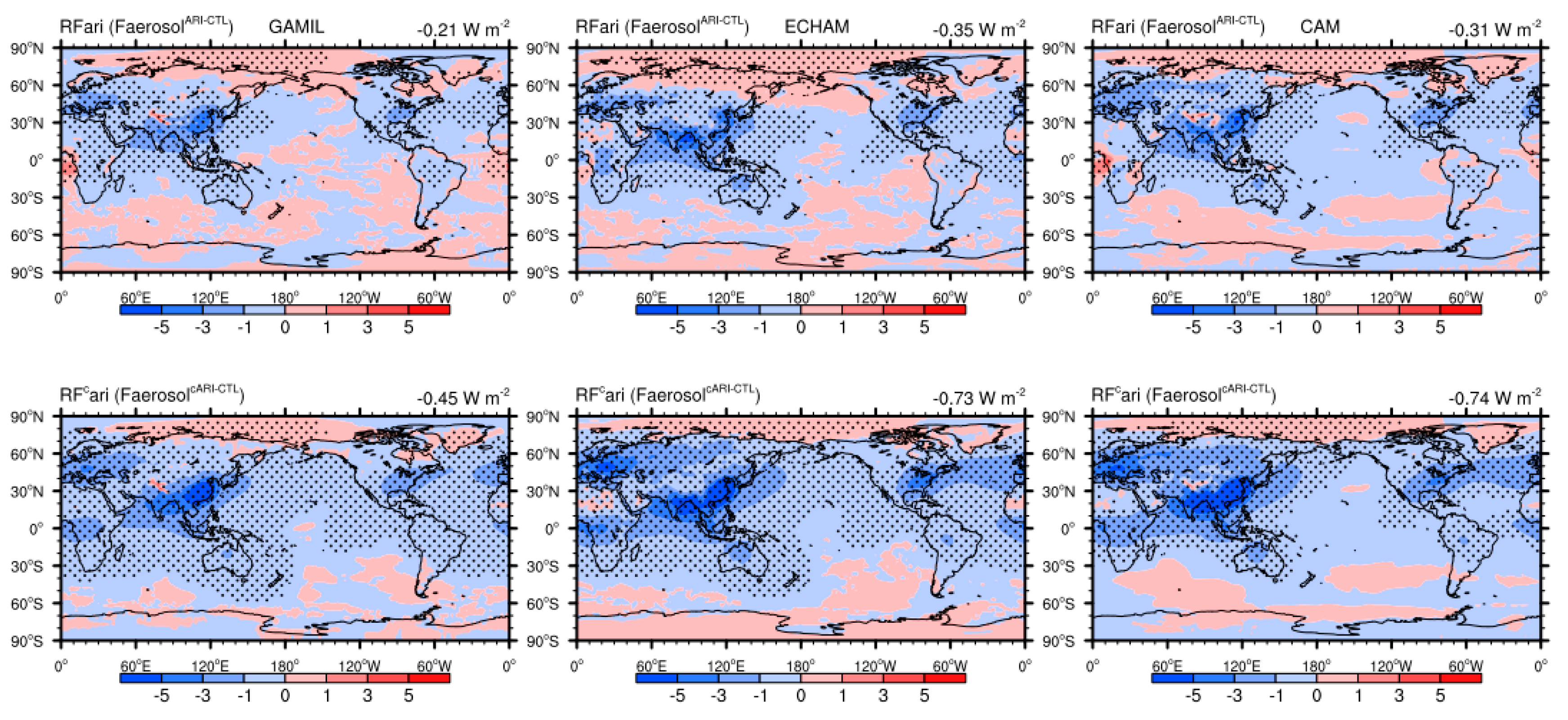
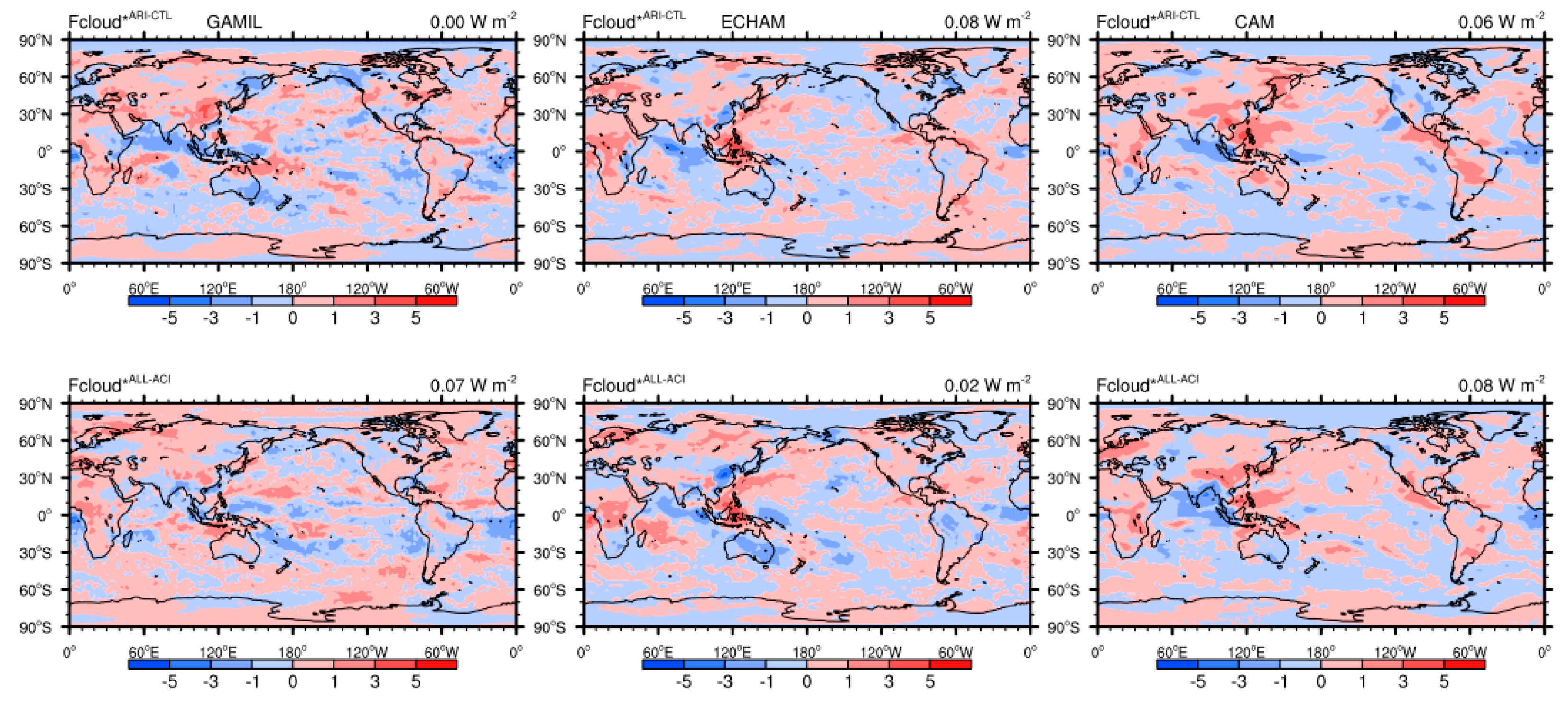
3.3. Contributions from “Ari”
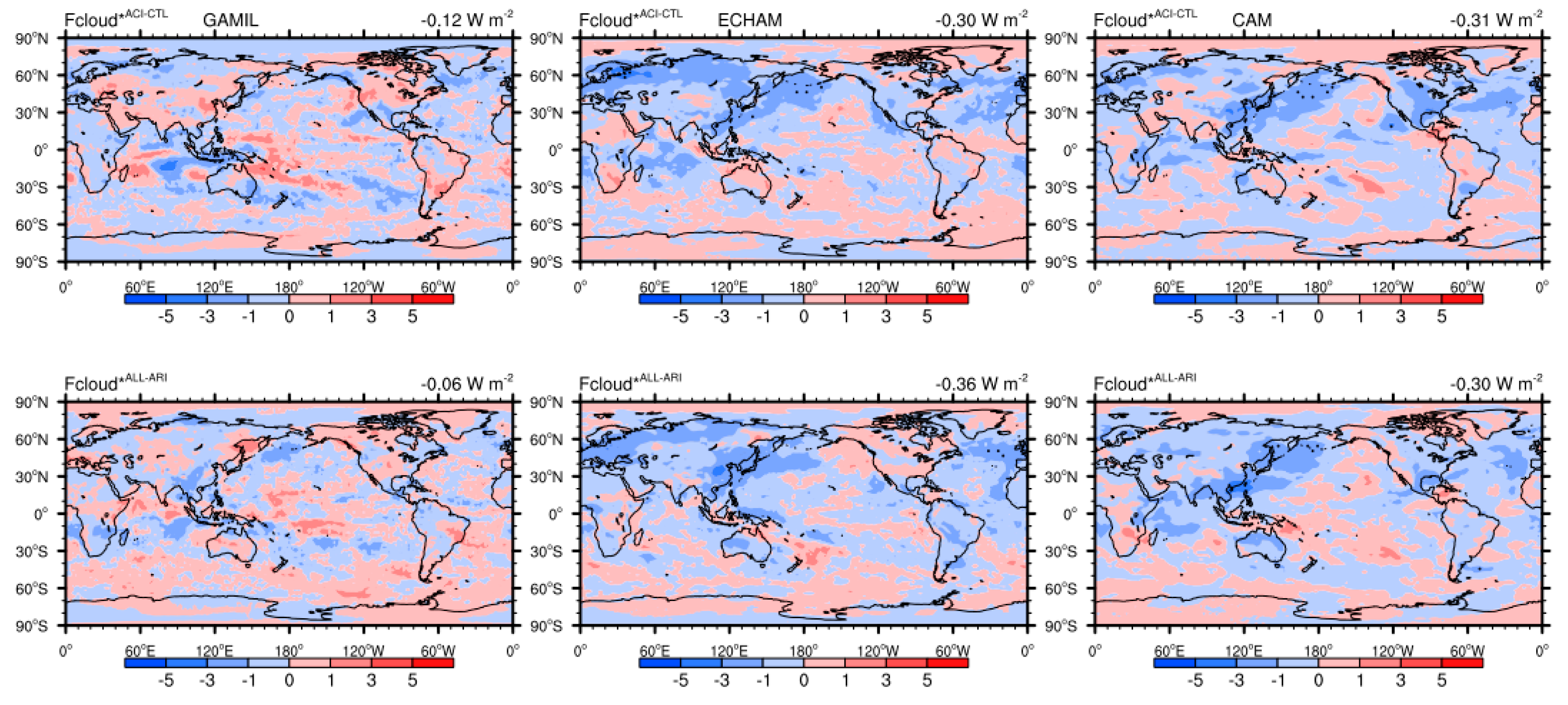
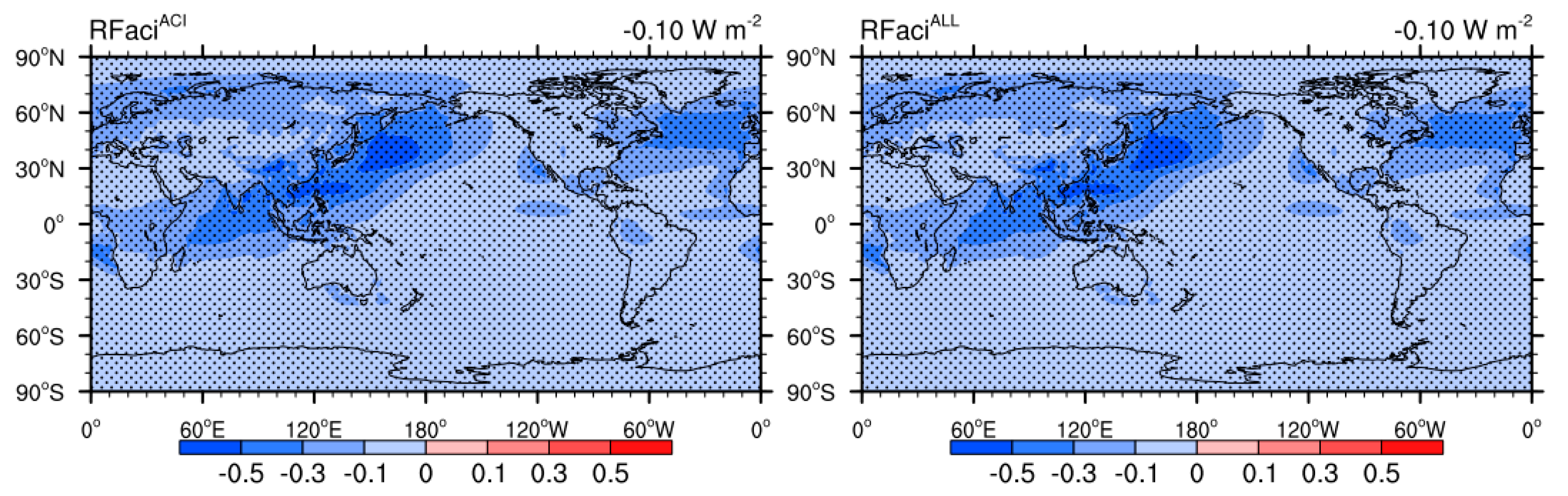
3.4. Contributions from “Aci”
4. Conclusions
Author Contributions
Funding
Acknowledgments
Conflicts of Interest
References
- Lohmann, U. Aerosol effects on clouds and climate. Space Sci. Rev. 2006, 125, 129–137. [Google Scholar] [CrossRef]
- Murphy, D.M.; Solomon, S.; Portmann, R.W.; Rosenlof, K.H.; Forster, P.M.; Wong, T. An observationally based energy balance for the Earth since 1950. J. Geophys. Res. Atmos. 2009, 114, D17107. [Google Scholar] [CrossRef]
- IPCC. Climate Change 2013: The Physical Science Basis; Cambridge University Press: Cambridge, UK, 2013; p. 1535. [Google Scholar]
- Myhre, G.; Myhre, C.E.L.; Samset, B.H.; Storelvmo, T. Aerosols and their Relation to Global Climate and Climate Sensitivity. Nat. Educ. Knowl. 2013, 4, 7. [Google Scholar]
- Myhre, G.; Shindell, D.; Bréon, F.M.; Collins, W.; Fuglestvedt, J.; Huang, J.; Koch, D.; Lamarque, J.F.; Lee, D.; Mendoza, B.; et al. Anthropogenic and Natural Radiative Forcing. In Climate Change 2013: The Physical Science Basis; Cambridge University Press: Cambridge, UK, 2013. [Google Scholar]
- Mielonen, T.; Laakso, A.; Karhunen, A.; Kokkola, H.; Partanen, A.I.; Korhonen, H.; Romakkaniemi, S.; Lehtinen, K.E.J. From nuclear power to coal power: Aerosol induced health and radiative effects. J. Geophys. Res. Atmos. 2015, 120, 12631–12643. [Google Scholar] [CrossRef]
- Eyring, V.; Bony, S.; Meehl, G.A.; Senior, C.A.; Stevens, B.; Stouffer, R.J.; Taylor, K.E. Overview of the Coupled Model Intercomparison Project Phase 6 (CMIP6) experimental design and organization. Geosci. Model Dev. 2016, 9, 1937–1958. [Google Scholar] [CrossRef]
- Regayre, L.A.; Johnson, J.S.; Yoshioka, M.; Pringle, K.J.; Sexton, D.M.H.; Booth, B.B.B.; Lee, L.A.; Bellouin, N.; Carslaw, K.S. Aerosol and physical atmosphere model parameters are both important sources of uncertainty in aerosol ERF. Atmos. Chem. Phys. 2018, 18, 9975–10006. [Google Scholar] [CrossRef]
- Irving, D.B.; Wijffels, S.; Church, J.A. Anthropogenic Aerosols, Greenhouse Gases, and the Uptake, Transport, and Storage of Excess Heat in the Climate System. Geophys. Res. Lett. 2019, 46, 4894–4903. [Google Scholar] [CrossRef]
- Lohmann, U.; Stier, P.; Hoose, C.; Ferrachat, S.; Kloster, S.; Roeckner, E.; Zhang, J. Cloud microphysics and aerosol indirect effects in the global climate model ECHAM5-HAM. Atmos. Chem. Phys. 2007, 7, 3425–3446. [Google Scholar] [CrossRef]
- Liu, X.; Easter, R.C.; Ghan, S.J.; Zaveri, R.; Rasch, P.; Shi, X.; Lamarque, J.F.; Gettelman, A.; Morrison, H.; Vitt, F.; et al. Toward a minimal representation of aerosols in climate models: Description and evaluation in the Community Atmosphere Model CAM5. Geosci. Model Dev. 2012, 5, 709–739. [Google Scholar] [CrossRef]
- Zhang, K.; O’Donnell, D.; Kazil, J.; Stier, P.; Kinne, S.; Lohmann, U.; Ferrachat, S.; Croft, B.; Quaas, J.; Wan, H.; et al. The global aerosol-climate model ECHAM-HAM, version 2: Sensitivity to improvements in process representations. Atmos. Chem. Phys. 2012, 12, 8911–8949. [Google Scholar] [CrossRef]
- Kirkevåg, A.; Iversen, T.; Seland, Ø.; Hoose, C.; Kristjánsson, J.E.; Struthers, H.; Ekman, A.M.; Ghan, S.; Griesfeller, J.; Nilsson, E.D.; et al. Aerosol-climate interactions in the norwegian earth system model—Noresm1-m. Geosci. Model Dev. 2013, 6, 207–244. [Google Scholar] [CrossRef]
- Boucher, O.; Randall, D.; Artaxo, P.; Bretherton, C.; Feingold, G.; Forster, P.; Kerminen, V.M.; Kondo, Y.; Liao, H.; Lohmann, U.; et al. Clouds and Aerosols. In Climate Change 2013: The Physical Science Basis; Cambridge University Press: Cambridge, UK, 2013. [Google Scholar]
- Carslaw, K.S.; Lee, L.A.; Reddington, C.L.; Pringle, K.J.; Rap, A.; Forster, P.M.; Mann, G.W.; Spracklen, D.V.; Woodhouse, M.T.; Regayre, L.A.; et al. Large contribution of natural aerosols to uncertainty in indirect forcing. Nature 2013, 503, 67–71. [Google Scholar] [CrossRef] [PubMed]
- Sanchez, K.J.; Roberts, G.C.; Calmer, R.; Nicoll, K.; Hashimshoni, E.; Rosenfeld, D.; Ovadnevaite, J.; Preissler, J.; Ceburnis, D.; O’Dowd, C.; et al. Top-down and bottom-up aerosol-cloud closure: Towards understanding sources of uncertainty in deriving cloud shortwave radiative flux. Atmos. Chem. Phys. 2017, 17, 9797–9814. [Google Scholar] [CrossRef]
- Ma, P.L.; Rasch, P.J.; Wang, M.; Wang, H.; Ghan, S.J.; Easter, R.C.; Gustafson, W.I.; Liu, X.; Zhang, Y.; Ma, H.Y. How does increasing horizontal resolution in a global climate model improve the simulation of aerosol-cloud interactions? Geophys. Res. Lett. 2015, 42, 5058–5065. [Google Scholar] [CrossRef]
- Weigum, N.; Schutgens, N.; Stier, P. Effect of aerosol subgrid variability on aerosol optical depth and cloud condensation nuclei: Implications for global aerosol modelling. Atmos. Chem. Phys. 2016, 16, 13619–13639. [Google Scholar] [CrossRef]
- Lee, S.S.; Li, Z.; Zhang, Y.; Yoo, H. Effects of model resolution and parameterizations on the simulations of clouds, precipitation, and their interactions with aerosols. Atmos. Chem. Phys. Discuss. 2017, 2017, 1–56. [Google Scholar] [CrossRef]
- Ghan, S.J.; Abdul-Razzak, H.; Nenes, A.; Ming, Y.; Liu, X.; Ovchinnikov, M.; Shipway, B.; Meskhidze, N.; Xu, J.; Shi, X. Droplet Nucleation: Physically-Based Parameterizations and Comparative Evaluation. J. Adv. Model. Earth Syst. 2011, 3. [Google Scholar] [CrossRef]
- Shindell, D.T.; Lamarque, J.F.; Schulz, M.; Flanner, M.; Jiao, C.; Chin, M.; Young, P.J.; Lee, Y.H.; Rotstayn, L.; Mahowald, N.; et al. Radiative forcing in the ACCMIP historical and future climate simulations. Atmos. Chem. Phys. 2013, 13, 2939–2974. [Google Scholar] [CrossRef]
- Stevens, B.; Fiedler, S.; Kinne, S.; Peters, K.; Rast, S.; Müsse, J.; Smith, S.J.; Mauritsen, T. MACv2-SP: A parameterization of anthropogenic aerosol optical properties and an associated Twomey effect for use in CMIP6. Geosci. Model Dev. 2017, 10, 433–452. [Google Scholar] [CrossRef]
- Stouffer, R.J.; Eyring, V.; Meehl, G.A.; Bony, S.; Senior, C.; Stevens, B.; Taylor, K.E. CMIP5 Scientific Gaps and Recommendations for CMIP6. Bull. Am. Meteorol. Soc. 2017, 98, 95–105. [Google Scholar] [CrossRef]
- Pascoe, C.; Lawrence, B.N.; Guilyardi, E.; Juckes, M.; Taylor, K.E. Designing and Documenting Experiments in CMIP6. Geosci. Model Dev. Discuss. 2019. in review. [Google Scholar] [CrossRef]
- Pincus, R.; Forster, P.M.; Stevens, B. The Radiative Forcing Model Intercomparison Project (RFMIP): Experimental protocol for CMIP6. Geosci. Model Dev. 2016, 9, 3447–3460. [Google Scholar] [CrossRef]
- Zhou, C.; Zelinka, M.D.; Klein, S.A. Impact of decadal cloud variations on the Earth’s energy budget. Nat. Geosci. 2016, 9, 871–874. [Google Scholar] [CrossRef]
- Ghan, S.; Wang, M.; Zhang, S.; Ferrachat, S.; Gettelman, A.; Griesfeller, J.; Kipling, Z.; Lohmann, U.; Morrison, H.; Neubauer, D.; et al. Challenges in constraining anthropogenic aerosol effects on cloud radiative forcing using present-day spatiotemporal variability. Proc. Natl. Acad. Sci. USA 2016, 113, 5804–5811. [Google Scholar] [CrossRef]
- Ceppi, P.; Brient, F.; Zelinka, M.D.; Hartmann, D.L. Cloud feedback mechanisms and their representation in global climate models. Wiley Interdiscip. Rev. Clim. Chang. 2017, 8, e465. [Google Scholar] [CrossRef]
- Fiedler, S.; Kinne, S.; Huang, W.T.; Räisänen, P.; O’Donnell, D.; Bellouin, N.; Stier, P.; Merikanto, J.; Noije, T.V.; Makkonen, R.; et al. Anthropogenic aerosol forcing—Insights from multiple estimates from aerosol-climate models with reduced complexity. Atmos. Chem. Phys. 2019, 19, 6821–6841. [Google Scholar] [CrossRef]
- Storelvmo, T.; Lohmann, U.; Bennartz, R. What governs the spread in shortwave forcings in the transient IPCC AR4 models? Geophys. Res. Lett. 2009, 36. [Google Scholar] [CrossRef]
- Lohmann, U.; Ferrachat, S. Impact of parametric uncertainties on the present-day climate and on the anthropogenic aerosol effect. Atmos. Chem. Phys. 2010, 10, 11373–11383. [Google Scholar] [CrossRef]
- Bond, T.C.; Doherty, S.J.; Fahey, D.W.; Forster, P.M.; Berntsen, T.; DeAngelo, B.J.; Flanner, M.G.; Ghan, S.; Kärcher, B.; Koch, D.; et al. Bounding the role of black carbon in the climate system: A scientific assessment. J. Geophys. Res. Atmos. 2013, 118, 5380–5552. [Google Scholar] [CrossRef]
- Fiedler, S.; Stevens, B.; Mauritsen, T. On the sensitivity of anthropogenic aerosol forcing to model-internal variability and parameterizing a Twomey effect. J. Adv. Model. Earth Syst. 2017, 9, 1325–1341. [Google Scholar] [CrossRef]
- Li, L.; Wang, B.; Wang, Y.; Wan, H. Improvements in Climate Simulation with Modifications to the Tiedtke Convective Parameterization in the Grid-Point Atmospheric Model of IAP LASG (GAMIL). Adv. Atmos. Sci. 2007, 24, 323–335. [Google Scholar] [CrossRef][Green Version]
- Li, L.; Lin, P.; Yu, Y.; Wang, B.; Zhou, T.; Liu, L.; Liu, J.; Bao, Q.; Xu, S.; Huang, W.; et al. The flexible global ocean-atmosphere-land system model, Grid-point Version 2: FGOALS-g2. Adv. Atmos. Sci. 2013, 30, 543–560. [Google Scholar] [CrossRef]
- Li, L.; Wang, B.; Dong, L.; Liu, L.; Shen, S.; Hu, N.; Sun, W.; Wang, Y.; Huang, W.; Shi, X.; et al. Evaluation of grid-point atmospheric model of IAP LASG version 2 (GAMIL2). Adv. Atmos. Sci. 2013, 30, 855–867. [Google Scholar] [CrossRef]
- Briegleb, B.P. Delta-Eddington approximation for solar radiation in the NCAR community climate model. J. Geophys. Res. Atmos. 1992, 97, 7603–7612. [Google Scholar] [CrossRef]
- Collins, W.D. A global signature of enhanced shortwave absorption by clouds. J. Geophys. Res. Atmos. 1998, 103, 31669–31679. [Google Scholar] [CrossRef]
- Shi, X.J.; Wang, B.; Liu, X.H.; Wang, M.H.; Li, L.J.; Dong, L. Aerosol Indirect Effects on Warm Clouds in the Grid-Point Atmospheric Model of IAP LASG (GAMIL). Atmos. Ocean. Sci. Lett. 2010, 3, 237–241. [Google Scholar]
- Shi, X.; Wang, B.; Liu, X.; Wang, M. Two-moment bulk stratiform cloud microphysics in the grid-point atmospheric model of IAP LASG (GAMIL). Adv. Atmos. Sci. 2013, 30, 868–883. [Google Scholar] [CrossRef]
- Cao, J.; Wang, B.; Yang, Y.M.; Ma, L.; Li, J.; Sun, B.; Bao, Y.; He, J.; Zhou, X.; Wu, L. The NUIST Earth System Model (NESM) version 3: Description and preliminary evaluation. Geosci. Model Dev. 2018, 11, 2975–2993. [Google Scholar] [CrossRef]
- Giorgetta, M.A.; Roeckner, E.; Mauritsen, T.; Stevens, B.; Bader, J.; Crueger, T.; Esch, M.; Rast, S.; Kornblueh, L.; Schmidt, H.; et al. The Atmospheric General Circulation Model ECHAM6–Model Description; Max Planck Institute for Meteorology: Hamburg, Germany, 2012. [Google Scholar]
- Lohmann, U.; Roeckner, E. Design and performance of a new cloud microphysics scheme developed for the ECHAM general circulation model. Clim. Dyn. 1996, 12, 557–572. [Google Scholar] [CrossRef]
- Gettelman, A.; Morrison, H.; Ghan, S.J. A new two-moment bulk stratiform cloud microphysics scheme in the community atmosphere model, version 3 (CAM3). Part II: Single-colunm and global results. J. Clim. 2008, 21, 3660–3679. [Google Scholar] [CrossRef]
- Morrison, H.; Gettelman, A. A new two-moment bulk stratiform cloud microphysics scheme in the community atmosphere model, version 3 (CAM3). Part I: Description and numerical tests. J. Clim. 2008, 21, 3642–3659. [Google Scholar] [CrossRef]
- Ghan, S.J.; Liu, X.; Easter, R.C.; Zaveri, R.; Rasch, P.J.; Yoon, J.H.; Eaton, B. Toward a Minimal Representation of Aerosols in Climate Models: Comparative Decomposition of Aerosol Direct, Semidirect, and Indirect Radiative Forcing. J. Clim. 2012, 25, 6461–6476. [Google Scholar] [CrossRef]
- Iacono, M.J.; Delamere, J.S.; Mlawer, E.J.; Shephard, M.W.; Clough, S.A.; Collins, W.D. Radiative forcing by long-lived greenhouse gases: Calculations with the AER radiative transfer models. J. Geophys. Res. Atmos. 2008, 113. [Google Scholar] [CrossRef]
- Sherwood, S.C.; Bony, S.; Boucher, O.; Bretherton, C.; Forster, P.M.; Gregory, J.M.; Stevens, B. Adjustments in the Forcing-Feedback Framework for Understanding Climate Change. Bull. Am. Meteorol. Soc. 2015, 96, 217–228. [Google Scholar] [CrossRef]
- Hansen, J. Efficacy of climate forcings. J. Geophys. Res. 2005, 110. [Google Scholar] [CrossRef]
- Ghan, S.J. Technical Note: Estimating aerosol effects on cloud radiative forcing. Atmos. Chem. Phys. 2013, 13, 9971–9974. [Google Scholar] [CrossRef]
- Nenes, A. Impacts of marine biogenic compounds on CCN properties, predicted cloud droplet number and indirect forcing. Geochim. Cosmochim. Acta 2009, 73, A937. [Google Scholar]
- Wang, M.; Ghan, S.; Ovchinnikov, M.; Liu, X.; Easter, R.; Kassianov, E.; Qian, Y.; Morrison, H. Aerosol indirect effects in a multi-scale aerosol-climate model PNNL-MMF. Atmos. Chem. Phys. 2011, 11, 5431–5455. [Google Scholar] [CrossRef]
- Twomey, S. The Influence of Pollution on the Shortwave Albedo of Clouds. J. Atmos. Sci. 1977, 34, 1149–1152. [Google Scholar] [CrossRef]
- Smith, C.J.; Kramer, R.J.; Myhre, G.; Forster, P.M.; Soden, B.J.; Andrews, T.; Boucher, O.; Faluvegi, G.; Flaschner, D.; Hodnebrog, O.; et al. Understanding Rapid Adjustments to Diverse Forcing Agents. Geophys. Res. Lett. 2018, 45, 12023–12031. [Google Scholar] [CrossRef]


| Names | Description |
|---|---|
| CTL | Simulation using model default pre-industrial times (PI, the year of 1850) aerosol forcings (i.e., anthropogenic aerosol forcings are excluded). |
| ARI | Same as CTL, but present-day (PD, the year of 2000) anthropogenic aerosol optical properties from the second version of the Max Planck Institute Aerosol Climatology (MACv2-SP) are considered. |
| ACI | Same as CTL, but PD anthropogenic aerosol Twomey effect from MACv2-SP is considered. |
| ALL | Same as CTL, but PD anthropogenic aerosol optical properties and Twomey effect from MACv2-SP are considered. |
| OLD | Same as CTL, but with model default PD aerosol forcings. |
| Names | Description |
|---|---|
| F (W∙m−2) | The all-sky shortwave net radiative fluxes at the top of the atmosphere (TOA). |
| Fc (W∙m−2) | The clear-sky F. |
| F* (W∙m−2) | Same as F, but calculated from radiation call without aerosol radiative effect. |
| Fc* (W∙m−2) | The clear-sky F*. |
| F# (W∙m−2) | Same as F, but derived from cloud optical properties without aerosol Twomey effect. |
| Faerosol (W∙m−2) | The shortwave aerosol forcing, Faerosol = F − F*. |
| Faerosolc (W∙m−2) | The clear-sky Faerosol, Faerosolc = Fc − Fc,*. |
| Fcloud (W∙m−2) | The shortwave cloud forcing, Fcloud = F − Fc. |
| Fcloud* (W∙m−2) | Fcloud without aerosol radiative effect, Fcloud*= F* − Fc,*. |
| dFcloud (W∙m−2) | The impact of aerosol radiative effect on calculating Fcloud, dFcloud = Fcloud − Fcloud*. |
| RFaci (W∙m−2) | The instantaneous aerosol Twomey effect, RFaci = F − F#. |
| AOD | The aerosol optical depth in the visible band. |
| AODa | The anthropogenic aerosol optical depth in the visible band calculated from MACv2-SP. |
| dN | The normalized change in drop number, calculated from MACv2-SP. |
| CLD (%) | The total cloud fraction. |
| LWP (g∙m−2) | The liquid water path. |
| CDNC (1010 m−2) | The background column-integrated grid-mean cloud droplet number concentration. |
| COD | The cloud optical depth in the visible band. |
| GAMIL | ECHAM | CAM | |||||||
|---|---|---|---|---|---|---|---|---|---|
| CTL | ALL | OLD | CTL | ALL | OLD | CTL | ALL | OLD | |
| −CTL | −CTL | −CTL | −CTL | −CTL | −CTL | ||||
| F | 237.98 | −0.27 | −1.98 | 239.35 | −0.63 | −0.21 | 240.34 | −0.54 | −2.22 |
| (0.10) | (0.06) | (0.08) | (0.09) | (0.06) | (0.06) | ||||
| F* | 243.72 | −0.06 | −2.04 | 241.82 | −0.30 | 0.04 | 241.79 | −0.25 | −2.15 |
| (0.10) | (0.06) | (0.08) | (0.09) | (0.06) | (0.06) | ||||
| Fc | 285.17 | −0.45 | −0.08 | 286.73 | −0.74 | −0.62 | 291.75 | −0.75 | −0.48 |
| (0.02) | (0.03) | (0.02) | (0.02) | (0.05) | (0.04) | ||||
| Fc* | 293.74 | −0.01 | −0.09 | 291.17 | −0.02 | 0.02 | 294.46 | −0.01 | −0.03 |
| (0.02) | (0.03) | (0.02) | (0.02) | (0.04) | (0.03) | ||||
| Faerosol | −5.74 | −0.21 | 0.06 | −2.47 | −0.33 | −0.26 | −1.49 | −0.29 | −0.07 |
| (0.01) | (0) | (0.01) | (0) | (0.01) | (0.01) | ||||
| Faerosolc | −8.58 | −0.45 | 0.01 | −4.44 | −0.73 | −0.65 | −2.70 | −0.74 | −0.45 |
| (0) | (0) | (0) | (0) | (0.01) | (0.01) | ||||
| Fcloud | −47.19 | 0.19 | −1.90 | −47.38 | 0.11 | 0.41 | −51.42 | 0.21 | −1.74 |
| (0.11) | (0.05) | (0.07) | (0.08) | (0.05) | (0.05) | ||||
| Fcloud* | −50.02 | −0.05 | −1.95 | −49.35 | −0.28 | 0.02 | −52.67 | −0.24 | −2.12 |
| (0.11) | (0.06) | (0.05) | (0.09) | (0.05) | (0.05) | ||||
| dFcloud | 2.83 | 0.24 | 0.06 | 1.97 | 0.39 | 0.39 | 1.25 | 0.44 | 0.38 |
| (0.01) | (0) | (0) | (0) | (0.01) | (0.01) | ||||
| AOD | 0.144 | 0.032 | 0 | 0.103 | 0.025 | 0.021 | 0.102 | 0.027 | 0.018 |
| (0) | (0) | (0) | (0) | (0.001) | (0.01) | ||||
| COD | 9.545 | 0.051 | 1.985 | 8.881 | 0.164 | −0.016 | 9.666 | 0.092 | 0.580 |
| (0.019) | (0.016) | (0.021) | (0.022) | (0.012) | (0.023) | ||||
| CLD | 54.22 | 0.03 | −0.07 | 62.42 | 0.04 | −0.01 | 63.83 | 0.02 | 0.29 |
| (0.07) | (0.03) | (0.05) | (0.07) | (0.05) | (0.05) | ||||
| LWP | 65.32 | −0.24 | 11.56 | 75.11 | 0.29 | 0.31 | 40.93 | −0.20 | 3.53 |
| (0.15) | (0.09) | (0.21) | (0.23) | (0.10) | (0.10) | ||||
| CDNC | 1.65 | −0.01 | 0.84 | 1.82 | 0 | 0 | 0.99 | 0 | 0.39 |
| (0) | (0) | (0) | (0) | (0) | (0) | ||||
| GAMIL | ECHAM | CAM | ||||
|---|---|---|---|---|---|---|
| ARI | ALL | ARI | ALL | ARI | ALL | |
| −CTL | −ACI | −CTL | −ACI | −CTL | −ACI | |
| F | −0.21 | −0.14 | −0.25 | −0.31 | −0.24 | −0.21 |
| (0.05) | (0.05) | (0.07) | (0.10) | (0.08) | (0.08) | |
| F* | 0 | 0.07 | 0.09 | 0.03 | 0.07 | 0.08 |
| (0.05) | (0.06) | (0.08) | (0.11) | (0.09) | (0.08) | |
| Fc | −0.45 | −0.45 | −0.71 | −0.72 | −0.74 | −0.73 |
| (0.02) | (0.02) | (0.02) | (0.02) | (0.04) | (0.03) | |
| Fc* | 0 | 0 | 0.02 | 0.01 | 0 | 0.01 |
| (0.02) | (0.02) | (0.02) | (0.02) | (0.04) | (0.04) | |
| Faerosol | −0.21 | −0.21 | −0.35 | −0.34 | −0.31 | −0.30 |
| (0) | (0) | (0) | (0.01) | (0.01) | (0.01) | |
| Faerosolc | −0.45 | −0.45 | −0.73 | −0.73 | −0.74 | −0.74 |
| (0) | (0) | (0) | (0) | (0.01) | (0.01) | |
| Fcloud | 0.24 | 0.30 | 0.46 | 0.41 | 0.50 | 0.51 |
| (0.05) | (0.05) | (0.07) | (0.10) | (0.07) | (0.08) | |
| Fcloud* | 0 | 0.07 | 0.08 | 0.02 | 0.06 | 0.08 |
| (0.05) | (0.05) | (0.07) | (0.10) | (0.07) | (0.08) | |
| dFcloud | 0.24 | 0.24 | 0.38 | 0.39 | 0.43 | 0.44 |
| (0) | (0) | (0) | (0) | (0) | (0.01) | |
| AOD | 0.032 | 0.032 | 0.025 | 0.025 | 0.027 | 0.027 |
| (0) | (0) | (0) | (0) | (0) | (0) | |
| COD | −0.037 | −0.044 | −0.034 | −0.011 | −0.018 | −0.027 |
| (0.022) | (0.012) | (0.017) | (0.020) | (0.020) | (0.026) | |
| CLD | 0.07 | 0.01 | −0.03 | 0.02 | −0.01 | 0 |
| (0.06) | (0.05) | (0.07) | (0.10) | (0.04) | (0.06) | |
| LWP | −0.20 | −0.23 | 0.17 | 0.36 | −0.04 | −0.11 |
| (0.10) | (0.09) | (0.17) | (0.19) | (0.08) | (0.12) | |
| CDNC | 0 | −0.01 | 0 | 0 | 0 | 0 |
| (0) | (0) | (0) | (0) | (0) | (0) | |
| GAMIL | ECHAM | CAM | ||||
|---|---|---|---|---|---|---|
| ACI | ALL | ACI | ALL | ACI | ALL | |
| −CTL | −ARI | −CTL | −ARI | −CTL | −ARI | |
| F | −0.12 | −0.06 | −0.32 | −0.37 | −0.33 | −0.30 |
| (0.08) | (0.13) | (0.08) | (0.06) | (0.07) | (0.05) | |
| F* | −0.12 | −0.06 | −0.32 | −0.39 | −0.33 | −0.32 |
| (0.08) | (0.14) | (0.08) | (0.06) | (0.07) | (0.06) | |
| Fc | −0.01 | −0.01 | −0.02 | −0.03 | −0.02 | −0.01 |
| (0.02) | (0.02) | (0.02) | (0.02) | (0.05) | (0.04) | |
| Fc* | −0.01 | 0 | −0.02 | −0.03 | −0.02 | −0.02 |
| (0.02) | (0.02) | (0.02) | (0.02) | (0.04) | (0.04) | |
| Faerosol | 0 | 0 | 0.01 | 0.02 | 0 | 0.02 |
| (0) | (0.01) | (0) | (0.01) | (0.01) | (0.01) | |
| Faerosolc | 0 | 0 | 0 | 0 | 0 | 0.01 |
| (0) | (0) | (0) | (0) | (0.01) | (0.01) | |
| Fcloud | −0.12 | −0.06 | −0.29 | −0.34 | −0.31 | −0.29 |
| (0.07) | (0.14) | (0.08) | (0.06) | (0.05) | (0.06) | |
| Fcloud* | −0.12 | −0.06 | −0.30 | −0.36 | −0.31 | −0.30 |
| (0.08) | (0.15) | (0.08) | (0.06) | (0.05) | (0.06) | |
| dFcloud | 0 | 0 | 0.01 | 0.02 | 0.01 | 0.01 |
| (0) | (0.01) | (0) | (0) | (0.01) | (0) | |
| AOD | 0 | 0 | 0 | 0 | 0 | 0 |
| (0) | (0) | (0) | (0) | (0.001) | (0.001) | |
| COD | 0.096 | 0.089 | 0.175 | 0.198 | 0.120 | 0.110 |
| (0.017) | (0.034) | (0.017) | (0.016) | (0.029) | (0.012) | |
| CLD | 0.02 | −0.04 | 0.02 | 0.07 | 0.02 | 0.03 |
| (0.04) | (0.10) | (0.09) | (0.09) | (0.06) | (0.04) | |
| LWP | −0.01 | −0.05 | −0.08 | 0.13 | 0.03 | −0.04 |
| (0.12) | (0.22) | (0.20) | (0.16) | (0.12) | (0.06) | |
| CDNC | 0 | 0 | 0 | 0 | 0 | 0 |
| (0) | (0.01) | (0) | (0) | (0) | (0) | |
| Names (Calculating Methods) | GAMIL | ECHAM | CAM |
|---|---|---|---|
| ERFall (FOLD−CTL) | −1.98 (0.06) | −0.21 (0.09) | −2.22 (0.06) |
| ERFari (FaerosolOLD−CTL) | 0.06 (0) | −0.26 (0) | −0.07 (0.01) |
| Fcloud*OLD−CTL | −1.95 (0.06) | 0.02 (0.09) | −2.12 (0.05) |
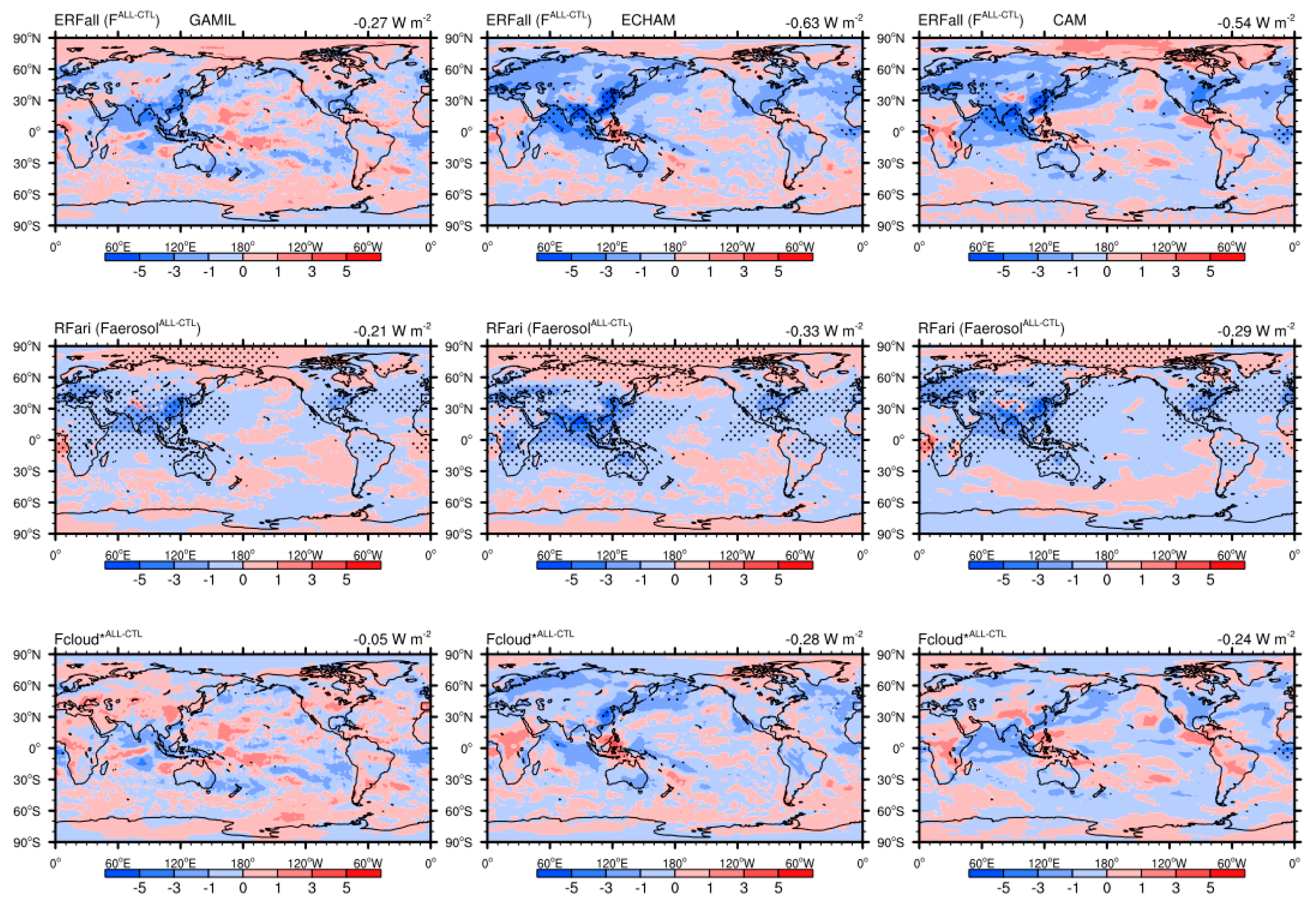
| ERFall (FALL−CTL) | −0.27 (0.10) | −0.63 (0.08) | −0.54 (0.06) |
| RFari (FaerosolALL−CTL) | −0.21 (0.01) | −0.33 (0.01) | −0.29 (0.01) |
| Fcloud*ALL−CTL | −0.05 (0.11) | −0.28 (0.05) | −0.24 (0.05) |
| ERFari (FARI−CTL) | −0.21 (0.05) | −0.25 (0.07) | −0.24 (0.08) |
| ERFari (FALL−ACI) | −0.14 (0.05) | −0.31 (0.10) | −0.21 (0.08) |
| ERFari (0.5FARI−CTL + 0.5FALL−ACI) | −0.18 | −0.28 | −0.23 |
| RFari (FaerosolARI−CTL) | −0.21 (0) | −0.35 (0) | −0.31 (0.01) |
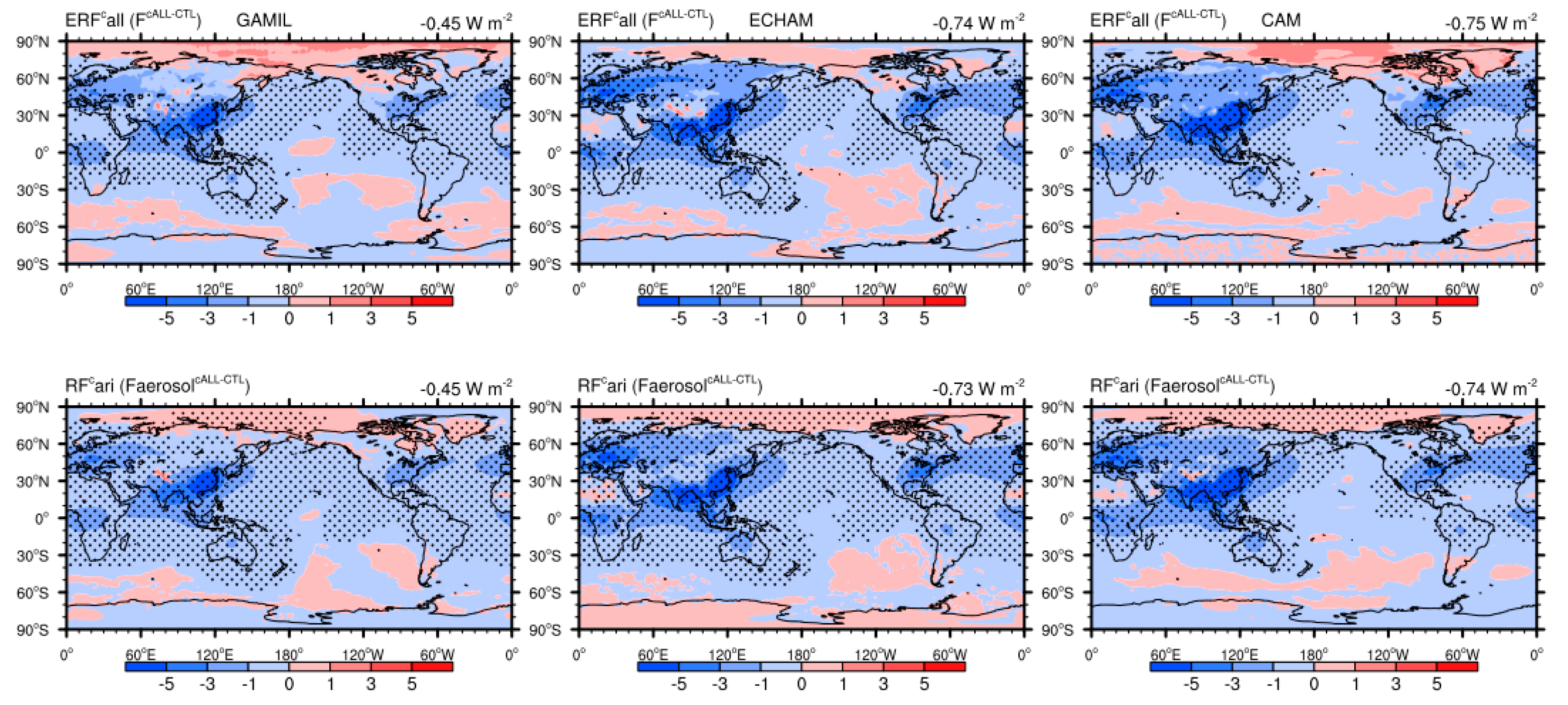
| RFari (FaerosolALL−ACI) | −0.21 (0) | −0.34 (0.01) | −0.30 (0.01) |
| RFari (0.5FaerosolARI−CTL + 0.5FaerosolALL−ACI) | −0.21 | −0.35 | −0.31 |
| Fcloud*ARI−CTL | 0 (0.05) | 0.08 (0.07) | 0.06 (0.07) |
| Fcloud*ALL−ACI | 0.07 (0.05) | 0.02 (0.10) | 0.08 (0.08) |
| 0.5Fcloud*ARI−CTL + 0.5Fcloud*ALL−ACI | 0.04 | 0.05 | 0.07 |
| ERFari (FACI−CTL) | −0.12 (0.08) | −0.32 (0.08) | −0.33 (0.07) |
| ERFari (FALL−ARI) | −0.06 (0.13) | −0.37 (0.06) | −0.30 (0.05) |
| ERFari (0.5FACI−CTL + 0.5FALL−ARI) | −0.09 | −0.35 | −0.32 |
| Fcloud*ACI−CTL | −0.12 (0.08) | −0.30 (0.08) | −0.31 (0.05) |
| Fcloud*ALL−ARI | −0.06 (0.15) | −0.36 (0.06) | −0.30 (0.06) |
| 0.5Fcloud*ACI−CTL + 0.5Fcloud*ALL−ARI | −0.09 | −0.33 | −0.31 |
© 2019 by the authors. Licensee MDPI, Basel, Switzerland. This article is an open access article distributed under the terms and conditions of the Creative Commons Attribution (CC BY) license (http://creativecommons.org/licenses/by/4.0/).
Share and Cite
Shi, X.; Zhang, W.; Liu, J. Comparison of Anthropogenic Aerosol Climate Effects among Three Climate Models with Reduced Complexity. Atmosphere 2019, 10, 456. https://doi.org/10.3390/atmos10080456
Shi X, Zhang W, Liu J. Comparison of Anthropogenic Aerosol Climate Effects among Three Climate Models with Reduced Complexity. Atmosphere. 2019; 10(8):456. https://doi.org/10.3390/atmos10080456
Chicago/Turabian StyleShi, Xiangjun, Wentao Zhang, and Jiaojiao Liu. 2019. "Comparison of Anthropogenic Aerosol Climate Effects among Three Climate Models with Reduced Complexity" Atmosphere 10, no. 8: 456. https://doi.org/10.3390/atmos10080456
APA StyleShi, X., Zhang, W., & Liu, J. (2019). Comparison of Anthropogenic Aerosol Climate Effects among Three Climate Models with Reduced Complexity. Atmosphere, 10(8), 456. https://doi.org/10.3390/atmos10080456