Appropriateness of Potential Evapotranspiration Models for Climate Change Impact Analysis in Yarlung Zangbo River Basin, China


Abstract
1. Introduction
2. Study Area and Data
2.1. Study Area
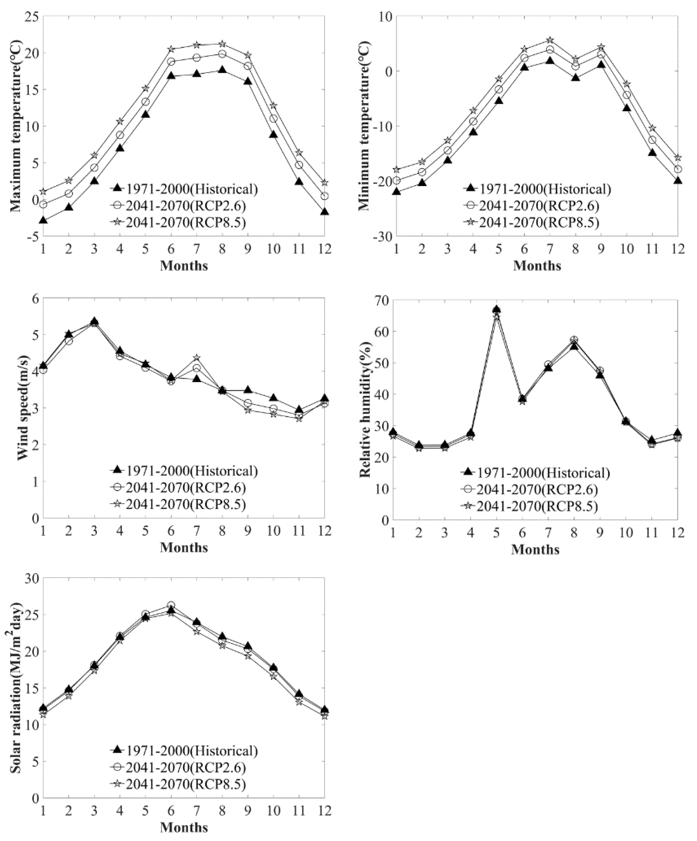
2.2. Data
3. Methodology
3.1. Methodology Framework
3.2. PET Models
3.2.1. FAO Penman-Monteith Model
3.2.2. Blaney-Criddle Model
3.2.3. Hargreaves Model
3.2.4. Makkink Model
3.2.5. Priestley-Taylor Model
3.3. Projection of Future PET and Performance Evaluation
3.4. Bias Correction Method
4. Results
4.1. Comparison of PET in the Baseline Period
4.2. Bias Correction Results for GCMs Data
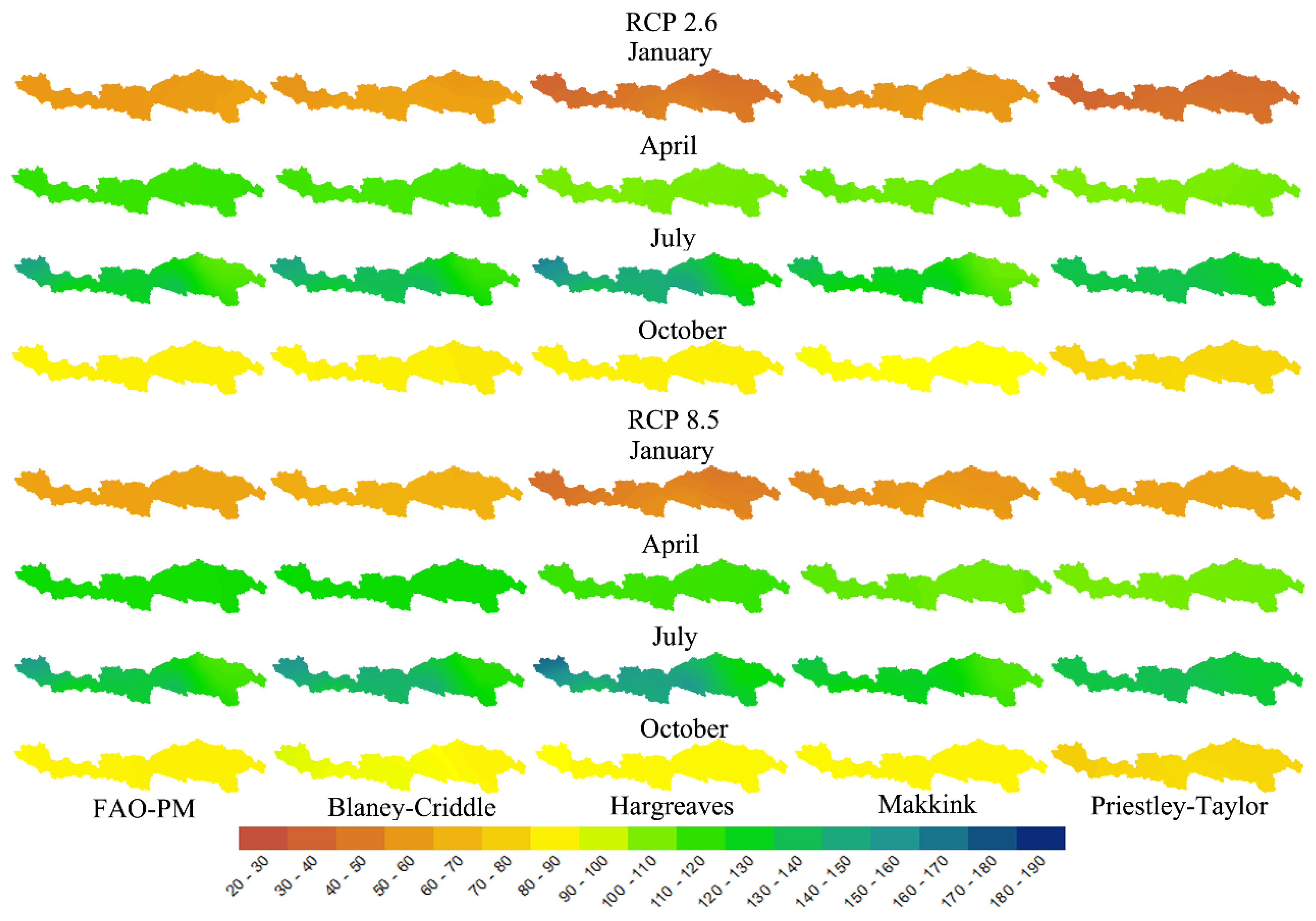
4.3. Changes in Annual, Seasonal and Monthly PET
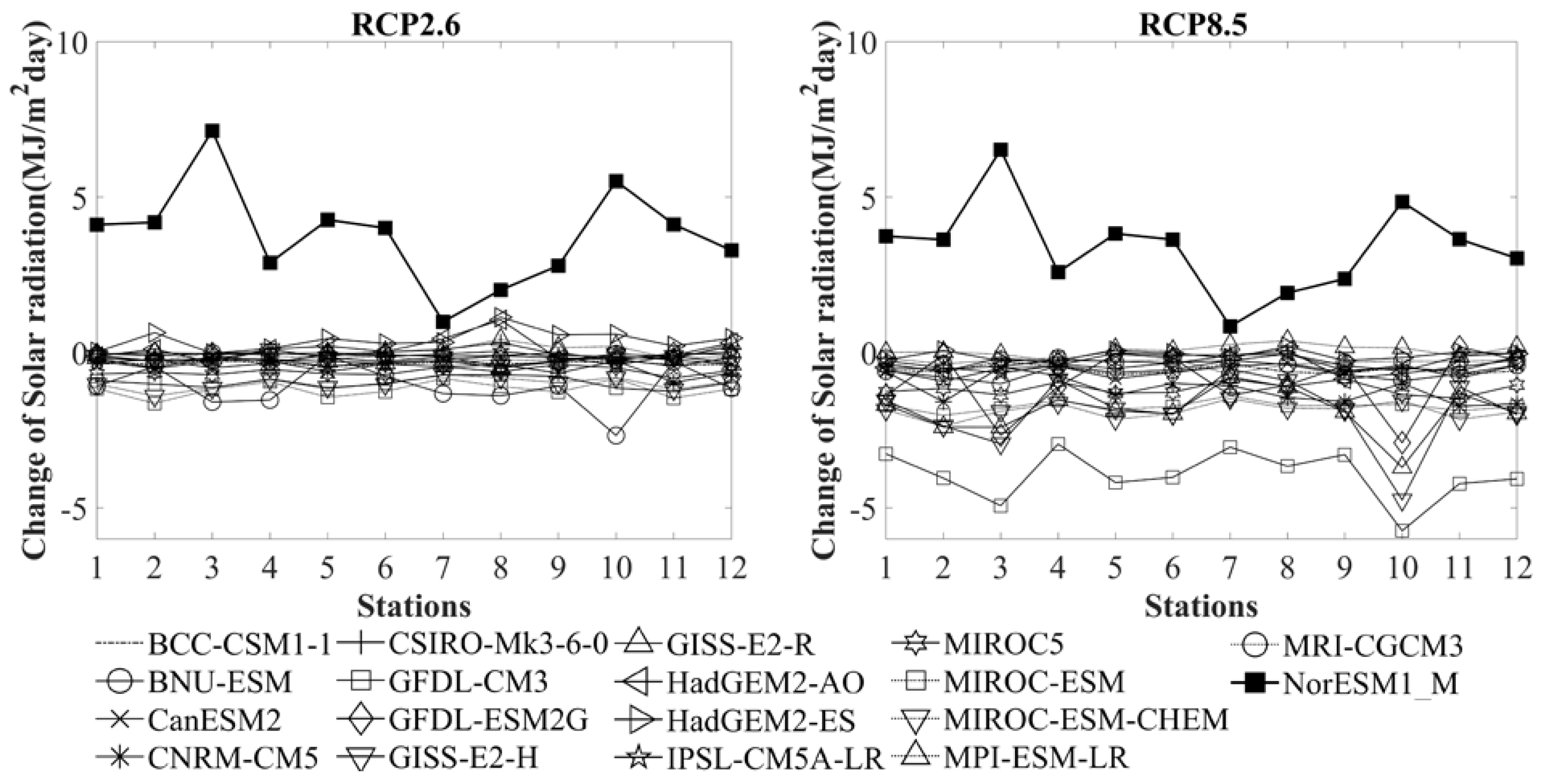
4.4. Uncertainty of Global Climate Models
5. Discussion
6. Conclusions
Supplementary Materials
Author Contributions
Funding
Acknowledgments
Conflicts of Interest
References
- Leal Filho, W.; Balogun, A.L.; Ayal, D.Y.; Bethurem, E.M.; Murambadoro, M.; Mambo, J.; Taddese, H.; Tefera, G.W.; Nagy, G.J.; Hubert, F.; et al. Strengthening climate change adaptation capacity in Africa-case studies from six major African cities and policy implications. Environ. Sci. Policy 2018, 86, 29–37. [Google Scholar] [CrossRef]
- Nam, W.; Hayes, M.J.; Svoboda, M.D.; Tadesse, T.; Wilhite, D.A. Drought hazard assessment in the context of climate change for South Korea. Agric. Water Manag. 2015, 160, 106–117. [Google Scholar] [CrossRef]
- Shi, H.; Chen, J.; Wang, K.; Niu, J. A new method and a new index for identifying socioeconomic drought events under climate change: A case study of the East River basin in China. Sci. Total Environ. 2018, 616, 363–375. [Google Scholar] [CrossRef] [PubMed]
- Trenberth, K.E.; Dai, A.; Van, D.; Schrier, G.; Jones, P.D.; Barichivich, J.; Briffa, K.R.; Sheffield, J. Global warming and changes in drought. Nat. Clim. Chang. 2014, 4, 17–22. [Google Scholar] [CrossRef]
- Arsiso, B.K.; Tsidu, G.M.; Stoffberg, G.H.; Tadesse, T. Climate change and population growth impacts on surface water supply and demand of Addis Ababa, Ethiopia. Clim. Risk Manag. 2017, 18, 21–33. [Google Scholar] [CrossRef]
- Mueller, N.D.; Gerber, J.S.; Johnston, M.; Ray, D.K.; Ramankutty, N.; Jonathan, A. Foley Closing yield gaps through nutrient and water management. Nature 2012, 490, 254–257. [Google Scholar] [CrossRef] [PubMed]
- Al-Saidi, M.; Elagib, N.A. Towards understanding the integrative approach of the water, energy and food nexus. Sci. Total Environ. 2017, 574, 1131–1139. [Google Scholar] [CrossRef]
- Acharjee, T.K.; Ludwig, F.; van Halsema, G.; Hellegers, P.; Supit, I. Future changes in water requirements of Boro rice in the face of climate change in North-West Bangladesh. Agric. Water Manag. 2017, 194, 172–183. [Google Scholar] [CrossRef]
- Singh, S.; Boote, K.J.; Angadi, S.V.; Grover, K.K. Estimating water balance, evapotranspiration and water use efficiency of spring safflower using the CROPGRO model. Agric. Water Manag. 2017, 185, 137–144. [Google Scholar] [CrossRef]
- Anapalli, S.S.; Green, T.R.; Reddy, K.N.; Gowda, P.H.; Sui, R.; Fisher, D.K.; Marek, G.W. Application of an energy balance method for estimating evapotranspiration in cropping systems. Agric. Water Manag. 2018, 204, 107–117. [Google Scholar] [CrossRef]
- McEvoy, D.J.; Huntington, J.L.; Mejia, J.F.; Hobbins, M.T. Improved seasonal drought forecasts using reference evapotranspiration anomalies. Geophys. Res. Lett. 2016, 43, 377–385. [Google Scholar] [CrossRef]
- Jaksa, W.T.; Sridhar, V. Effect of irrigation in simulating long-term evapotranspiration climatology in a human-dominated river basin system. Agric. For. Meteorol. 2015, 200, 109–118. [Google Scholar] [CrossRef]
- Ozturk, O.F.; Shukla, M.K.; Stringam, B.; Picchioni, G.A.; Gard, C. Irrigation with brackish water changes evapotranspiration, growth and ion uptake of halophytes. Agric. Water Manag. 2018, 195, 142–153. [Google Scholar] [CrossRef]
- Yao, Y.; Liang, S.; Li, X.; Chen, J.; Liu, S.; Jia, K.; Pan, M. Improving global terrestrial evapotranspiration estimation using support vector machine by integrating three process-based algorithms. Agric. Meteorol. 2017, 242, 55–74. [Google Scholar] [CrossRef]
- Guo, D.; Westra, S.; Maier, H.R. An R package for modelling actual, potential and reference evapotranspiration. Environ. Model. Softw. 2016, 78, 216–224. [Google Scholar] [CrossRef]
- Li, S.; Kang, S.; Zhang, L.; Zhang, J.; Du, T.; Tong, L.; Ding, R. Evaluation of six potential evapotranspiration models for estimating crop potential and actual evapotranspiration in arid regions. J. Hydrol. 2016, 543, 450–461. [Google Scholar] [CrossRef]
- Zheng, H.; Yu, G.; Wang, Q.; Zhu, X.; Yan, J.; Wang, H.; Shi, P.; Zhao, F.; Li, Y.; Zhao, L.; et al. Assessing the ability of potential evapotranspiration models in capturing dynamics of evaporative demand across various biomes and climatic regimes with ChinaFLUX measurements. J. Hydrol. 2017, 551, 70–80. [Google Scholar] [CrossRef]
- Milly, P.C.D.; Dunne, K.A. Potential evapotranspiration and continental drying. Nat. Clim. Chang. 2016, 6, 946–949. [Google Scholar] [CrossRef]
- Liu, X.; Xu, C.; Zhong, X.; Li, Y.; Yuan, X.; Cao, J.F. Comparison of 16 models for reference crop evapotranspiration against weighing lysimeter measurement. Agric. Water Manag. 2017, 184, 145–155. [Google Scholar] [CrossRef]
- Muniandy, J.M.; Yusop, Z.; Askari, M. Evaluation of reference evapotranspiration models and determination of crop coefficient for Momordica charantia and Capsicum annuum. Agric. Water Manag. 2016, 169, 77–89. [Google Scholar] [CrossRef]
- Constantin, J.; Willaume, M.; Murgue, C.; Lacroix, B.; Therond, O. The soil-crop models STICS and AqYield predict yield and soil water content for irrigated crops equally well with limited data. Agriclutural Meteorol. 2015, 206, 55–68. [Google Scholar] [CrossRef]
- Gentilucci, M.; Barbieri, M.; Burt, P. Exploring the Nexus of Geoecology, Geography, Geoarcheology and Geotourism: Advances and Applications for Sustainable Development in Environmental Sciences and Agroforestry Research. In Climate and Territorial Suitability for the Vineyards Developed Using GIS Techniques; Springer: Basel, Switzerland, 2018; pp. 11–13. [Google Scholar]
- Zohry, A.E.H.; Ouda, S.A. Management of Climate Induced Drought and Water Scarcity in Egypt. Upper Egypt: Management of high water consumption crops by intensification. In Management of Climate Induced Drought and Water Scarcity in Egypt; Springer: Basel, Switzerland, 2016; pp. 63–76. [Google Scholar]
- Blaney, H.F.; Criddle, W.D. Determining Water Requirements in Irrigated Areas from Climatological Irrigation Data; U.S. Soil Conservation Service: Washington, DC, USA, 1950; Volume 48.
- Makkink, G.F. Testing the Penman formula by means of lysimeters. J. Inst. Water Eng. 1957, 11, 277–288. [Google Scholar]
- Rohwer, C. Evaporation from free water surface. Usda Tech. Null. 1931, 217, 1–96. [Google Scholar]
- Allen, R.G.; Smith, M.; Perrier, A.; Pereira, L.S. An update for the calculation of Potential evapotranspiration. ICID Bull. 1994, 43, 35–92. [Google Scholar]
- Aouissi, J.; Benabdallah, S.; Chabaane, Z.L.; Cudennec, C. Evaluation of potential evapotranspiration assessment methods for hydrological modelling with SWAT-Application in data-scarce rural Tunisia. Agric. Water Manag. 2016, 174, 39–51. [Google Scholar] [CrossRef]
- Feng, Y.; Jia, Y.; Cui, N.; Zhao, L.; Li, C.; Gong, D. Calibration of Hargreaves model for reference evapotranspiration estimation in Sichuan basin of southwest China. Agric. Water Manag. 2017, 181, 1–9. [Google Scholar] [CrossRef]
- Minacapilli, M.; Cammalleri, C.; Ciraolo, G.; Rallo, G.; Provenzano, G. Using scintillometry to assess reference evapotranspiration methods and their impact on the water balance of olive groves. Agric. Water Manag. 2016, 170, 49–60. [Google Scholar] [CrossRef]
- Douglas, E.M.; Jacobs, J.M.; Sumner, D.M.; Ray, R.L. A comparison of models for estimating potential evapotranspiration for Florida land cover types. J. Hydrol. 2009, 373, 366–376. [Google Scholar] [CrossRef]
- Ji, X.B.; Chen, J.M.; Zhao, W.Z.; Kang, E.S.; Jin, B.W.; Xu, S.Q. Comparison of hourly and daily Penman-Monteith grass- and alfalfa-reference evapotranspiration equations and crop coefficients for maize under arid climatic conditions. Agric. Water Manag. 2017, 192, 1–11. [Google Scholar] [CrossRef]
- Perera, K.C.; Western, A.W.; Nawarathna, B.; George, B. Comparison of hourly and daily reference crop evapotranspiration equations across seasons and climate zones in Australia. Agric. Water Manag. 2015, 148, 84–96. [Google Scholar] [CrossRef]
- Xu, C.Y.; Singh, V.P. Evaluation and generalization of temperature-based methods for calculating evaporation. Hydrol. Process. 2001, 15, 305–319. [Google Scholar] [CrossRef]
- Liu, X.; Li, Y.; Wang, O. Evaluation on several temprature-based methods for estimating reference crop evapotranspiration. Trans. Chin. Soc. Agric. Eng. 2006, 22, 12–18. [Google Scholar]
- Yao, T.D.; Thompson, L.; Yang, W.; Yu, W.S.; Gao, Y.; Guo, X.J.; Yang, X.X.; Duan, K.Q.; Zhao, H.B.; Xu, B.Q.; et al. Different glacier status with atmospheric circulations in Tibetan Plateau and surroundings. Nat. Clim. Chang. 2012, 2, 663–667. [Google Scholar] [CrossRef]
- Maraun, D.; Shepherd, T.G.; Widmann, M.; Zappa, G.; Walton, D.; Gutiérrez, J.M.; Hagemann, S.; Richter, I.; Soares, P.M.M.; Hall, A.; et al. Towards process-informed bias correction of climate change simulations. Nat. Clim. Chang. 2017, 7, 764–773. [Google Scholar] [CrossRef]
- Fang, G.H.; Yang, J.; Chen, Y.N.; Zammit, C. Comparing bias correction methods in downscaling meteorological variables for a hydrologic impact study in an arid area in China. Hydrol. Earth Syst. Sci. 2015, 19, 2547–2559. [Google Scholar] [CrossRef]
- Teutschbein, C.; Seibert, J. Bias correction of regional climate model simulations for hydrological climate-change impact studies: Review and evaluation of different methods. J. Hydrol. 2012, 456, 12–29. [Google Scholar] [CrossRef]
- Thompson, J.R.; Crawley, A.; Kingston, D.G. GCM-related uncertainty for river flows and inundation under climate change: The Inner Niger Delta. Hydrol. Sci. J.Des Sci. Hydrol. 2016, 61, 2325–2347. [Google Scholar] [CrossRef]
- Flannigan, M.D.; Wotton, B.M.; Marshall, G.A.; De Groot, W.J.; Johnston, J.; Jurko, N.; Cantin, A.S. Fuel moisture sensitivity to temperature and precipitation: climate change implications. Clim. Chang. 2016, 134, 59–71. [Google Scholar] [CrossRef]
- Sorribas, M.V.; Paiva, R.C.; Melack, J.M.; Bravo, J.M.; Jones, C.; Carvalho, L.; Costa, M.H. Projections of climate change effects on discharge and inundation in the Amazon basin. Clim. Chang. 2016, 136, 555–570. [Google Scholar] [CrossRef]
- Ramirez-Villegas, J.; Challinor, A.J.; Thornton, P.K.; Jarvis, A. Implications of regional improvement in global climate models for agricultural impact research. Environ. Res. Lett. 2013, 8, 024018. [Google Scholar] [CrossRef]
- Smith, P.C.; Heinrich, G.; Suklitsch, M.; Gobiet, A.; Stoffel, M.; Fuhrer, J. Station-scale bias correction and uncertainty analysis for the estimation of irrigation water requirements in the Swiss Rhone catchment under climate change. Clim. Chang. 2014, 127, 521–534. [Google Scholar] [CrossRef]
- Zhang, X.; Booij, M.J.; Xu, Y. Improved Simulation of Peak Flows under Climate Change: Postprocessing or Composite Objective Calibration? J. Hydrometeorol. 2015, 16, 2187–2208. [Google Scholar] [CrossRef]
- Teng, J.; Potter, N.J.; Chiew, F.H.S.; Zhang, L.; Wang, B.; Vaze, J.; Evans, J.P. How does bias correction of regional climate model precipitation affect modelled runoff? Hydrol. Earth Syst. Sci. 2015, 19, 711–728. [Google Scholar] [CrossRef]
- Raty, O.; Raisanen, J.; Ylhaisi, J.S. Evaluation of delta change and bias correction methods for future daily precipitation: intermodel cross-validation using ENSEMBLES simulations. Clim. Dyn. 2014, 42, 2287–2303. [Google Scholar] [CrossRef]
- Grillakis, M.G.; Koutroulis, A.G.; Tsanis, I.K. Multisegment statistical bias correction of daily GCM precipitation output. J. Geophys. Res. Atmos. 2013, 118, 3150–3162. [Google Scholar] [CrossRef]
- Gao, Z.; He, J.; Dong, K.; Bian, X.; Li, X. Sensitivity study of reference crop evapotranspiration during growing season in the West Liao River basin, China. Theor. Appl. Climatol. 2016, 124, 865–881. [Google Scholar] [CrossRef]
- Gong, L.; Xu, C.; Chen, D.; Halldin, S.; Chen, Y.D. Sensitivity of the Penman-Monteith reference evapotranspiration to key climatic variables in the Changjiang (Yangtze River) basin. J. Hydrol. 2006, 329, 620–629. [Google Scholar] [CrossRef]
- Ma, D.; Wang, T.; Gao, C.; Pan, S.; Sun, Z.; Xu, Y.P. Potential evapotranspiration changes in Lancang River Basin and Yarlung Zangbo River Basin, southwest China. Hydrol. Sci. J. 2018, 63, 1653–1668. [Google Scholar] [CrossRef]
- Xu, Y.; Pan, S.; Fu, G.; Tian, Y.; Zhang, X. Future potential evapotranspiration changes and contribution analysis in Zhejiang Province, East China. J. Geophys. Res. Atmos. 2014, 119, 2174–2192. [Google Scholar] [CrossRef]
- Themessl, M.J.; Gobiet, A.; Leuprecht, A. Empirical-statistical downscaling and error correction of daily precipitation from regional climate models. Int. J. Climatol. 2011, 31, 1530–1544. [Google Scholar] [CrossRef]
- Haddeland, I.; Heinke, J.; Voß, F.; Eisner, S.; Chen, C.; Hagemann, S.; Ludwig, F. Effects of climate model radiation, humidity and wind estimates on hydrological simulations. Hydrol. Earth Syst. Sci. 2012, 16, 305–318. [Google Scholar] [CrossRef]
- Kottek, M.; Grieser, J.; Beck, C.; Rudolf, B.; Rubel, F. World Map of the Köppen-Geiger climate classification updated. Meteorol. Z. 2006, 15, 259–263. [Google Scholar] [CrossRef]
- Caesar, J.; Janes, T.; Lindsay, A.; Bhaskaran, B. Temperature and precipitation projections over Bangladesh and the upstream Ganges, Brahmaputra and Meghna systems. Environ. Sci. Process. Impacts 2015, 17, 1047–1056. [Google Scholar] [CrossRef] [PubMed]
- Shi, Y.; Gao, X.; Zhang, D.; Giorgi, F. Climate change over the Yarlung Zangbo-Brahmaputra River Basin in the 21st century as simulated by a high resolution regional climate model. Quat. Int. 2011, 244, 159–168. [Google Scholar] [CrossRef]
- Wei, Y.; Fang, Y. Spatio-temporal characteristics of global warming in the Tibetan Plateau during the last 50 years based on a generalised temperature zone-elevation model. Plos ONE 2013, 8, 60044. [Google Scholar] [CrossRef] [PubMed]
- Wu, S.; Yin, Y.; Zheng, D.; Yang, Q. Moisture conditions and climate trends in China during the period 1971–2000. Int. J. Climatol. J. R. Meteorol. Soc. 2006, 26, 193–206. [Google Scholar] [CrossRef]
- Hargreaves, G.H.; Samni, Z.A. Estimation of potential evapotranspiration. Journal of Irrigation and Drainage Division. Proc. Am. Soc. Civ. Eng. 1982, 108, 223–230. [Google Scholar]
- Hargreaves, G.H.; Samni, Z.A. Reference crop evapotranspiration from temperature. Trans. Am. Soc. Agric. Eng. 1985, 1, 96–99. [Google Scholar] [CrossRef]
- Hansen, S. Estimation of potential and actual evapotranspiration. Nordic Hydrol. 1984, 15, 205–212. [Google Scholar] [CrossRef]
- Rahimikhoob, A.; Behbahani, M.R.; Fakheri, J. An Evaluation of Four Reference Evapotranspiration Models in a Subtropical Climate. Water Resour. Manag. 2012, 26, 2867–2881. [Google Scholar] [CrossRef]
- Cristea, N.C.; Kampf, S.K.; Burges, S.J. Revised Coefficients for Priestley-Taylor and Makkink-Hansen Equations for Estimating Daily Reference Evapotranspiration. J. Hydrol. Eng. 2013, 18, 1289–1300. [Google Scholar] [CrossRef]
- Tabari, H. Evaluation of Reference Crop Evapotranspiration Equations in Various Climates. Water Resour. Manag. 2010, 24, 2311–2337. [Google Scholar] [CrossRef]
- Priestley, C.H.B.; Taylor, R.J. On the assessment of the surface heat flux and evaporation using large-scale parameters. Mon. Weather. Rev. 1972, 100, 81–92. [Google Scholar] [CrossRef]
- Teutschbein, C.; Seibert, J. Is bias correction of regional climate model (RCM) simulations possible for non-stationary conditions? Hydrol. Earth Syst. Sci. 2013, 17, 5061–5077. [Google Scholar] [CrossRef]
- Shrestha, B.; Maskey, S.; Babel, M.S.; van Griensven, A.; Uhlenbrook, S. Sediment related impacts of climate change and reservoir development in the Lower Mekong River Basin: A case study of the Nam Ou Basin, Lao PDR. Clim. Chang. 2018, 149, 13–27. [Google Scholar] [CrossRef]
- Wilcke, R.A.I.; Mendlik, T.; Gobiet, A. Multi-variable error correction of regional climate models. Clim. Chang. 2013, 120, 871–887. [Google Scholar] [CrossRef]
- Xuan, W.; Ma, C.; Kang, L.; Gu, H.; Pan, S.; Xu, Y.P. Evaluating historical simulations of CMIP5 GCMs for key climatic variables in Zhejiang Province, China. Theor. Appl. Climatol. 2015, 128, 207–222. [Google Scholar] [CrossRef]
- Yang, W.; Gardelin, M.; Olsson, J.; Bosshard, T. Multi-variable bias correction: application of forest fire risk in present and future climate in Sweden. Nat. Hazards Earth Syst. Sci. 2015, 15, 2037–2057. [Google Scholar] [CrossRef]
- Yan, D.; Werners, S.E.; Ludwig, F.; Huang, H.Q. Hydrological response to climate change: The Pearl River, China under different RCP scenarios. J. Hydrol. Reg. Stud. 2015, 4, 228–245. [Google Scholar] [CrossRef]
- Traore, B.; Descheemaeker, K.; Van Wijk, M.T.; Corbeels, M.; Supit, I.; Giller, K.E. Modelling cereal crops to assess future climate risk for family food self-sufficiency in southern Mali. FIELD Crop. Res. 2017, 201, 133–145. [Google Scholar] [CrossRef]
- Gebre, S.L.; Ludwig, F. Hydrological response to climate change of the upper blue Nile River Basin: based on IPCC fifth assessment report (AR5). J. Climatol. Weather. Forecast. 2015, 3, 121. [Google Scholar]


| No. | GCMs | Developer Resolution (lat. × lon.) | |
|---|---|---|---|
| 1 | BCC-CSM1-1 | Beijing Climate Center, China Meteorological Administration, China | ~2.8125° × 2.8125° |
| 2 | BNU-ESM | Beijing Normal University, China | ~2.8125° × 2.8125° |
| 3 | CanESM2 | Canadian Centre for Climate Modelling and Analysis, Canada | ~2.8125° × 2.8125° |
| 4 | CNRM-CM5 | CNRM/CeatreEuropeen de Recherche et Formation Avabcees en Calcul Scientifique, France | ~1.406° × 1.406° |
| 5 | CSIRO-Mk3-6-0 | CSIRO in collaboration with Queensland Climate Change Centre of Excellence, Australia | ~1.875° × 1.875° |
| 6 | GFDL-CM3 | Geophysical Fluid Dynamics Laboratory, National Oceanic and Atmospheric Administration, USA | ~2° × 2.5° |
| 7 | GFDL-ESM2G | Geophysical Fluid Dynamics Laboratory, National Oceanic and Atmospheric Administration, USA | ~2° × 2.5° |
| 8 | GISS-E2-H | GISS, National Aeronautics and Space Administration. USA | ~2° × 2.5° |
| 9 | GISS-E2-R | GISS, National Aeronautics and Space Administration. USA | ~2° × 2.5° |
| 10 | HadGEM2-AO | Met Office Hadley Centre, UK | ~1.241° × 1.875° |
| 11 | HadGEM2-ES | Met Office Hadley Centre, UK | ~1.241° × 1.875° |
| 12 | IPSL-CM5A-LR | Institute Pierre-Simon Laplace, France | ~1.875° × 3.75° |
| 13 | MIROC5 | National Institute for Environmental Studies, Japan | ~1.406° × 1.406° |
| 14 | MIROC-ESM | National Institute for Environmental Studies, Japan | ~1.406° × 1.406° |
| 15 | MIROC-ESM-CHEM | National Institute for Environmental Studies, Japan | ~1.406° × 1.406° |
| 16 | MPI-ESM-LR | Max Planck Institute for Meteorology, Germany | ~1.875° × 1.875° |
| 17 | MRI-CGCM3 | Meteorological Research Institute, Japan | ~1.125° × 1.125° |
| 18 | NorESM1_M | Norwegian Climate Centre, Norwegian | ~1.89° × 2.5° |
| Models | Blaney-Criddle | Hargreaves | Makkink | Priestley-Taylor | |||||
|---|---|---|---|---|---|---|---|---|---|
| Original | Stations | No. | 0.85 (0.5–1.2) | 0.0023 | 0.7 | 1.26 | |||
| MAM | JJA | SON | DJF | Annual | Annual | Annual | |||
| Calibrated | Dangxiong | 1 | 1.16 | 0.91 | 0.89 | 1.20 | 0.0025 | 0.62 | 1.09 |
| Dingri | 2 | 1.34 | 0.97 | 1.01 | 1.35 | 0.0026 | 0.65 | 1.17 | |
| Gaize | 3 | 1.37 | 1.12 | 1.18 | 1.70 | 0.0028 | 0.69 | 1.2 | |
| Jiali | 4 | 1.05 | 0.85 | 0.85 | 1.17 | 0.0023 | 0.61 | 1.03 | |
| Jiangzi | 5 | 1.23 | 0.93 | 0.95 | 1.19 | 0.0024 | 0.65 | 1.16 | |
| Lasa | 6 | 1.07 | 0.89 | 0.84 | 0.96 | 0.0024 | 0.66 | 1.19 | |
| Linzhi | 7 | 0.81 | 0.70 | 0.68 | 0.74 | 0.002 | 0.66 | 1.12 | |
| Longzi | 8 | 1.12 | 0.90 | 0.91 | 1.02 | 0.0024 | 0.66 | 1.17 | |
| Nielamu | 9 | 0.96 | 0.78 | 0.80 | 1.02 | 0.0026 | 0.58 | 0.99 | |
| Pulan | 10 | 1.23 | 0.98 | 1.07 | 1.17 | 0.0027 | 0.64 | 0.98 | |
| Rikaze | 11 | 1.16 | 0.90 | 0.86 | 1.09 | 0.0023 | 0.64 | 1.15 | |
| Zedang | 12 | 1.13 | 0.91 | 0.89 | 1.0 | 0.0024 | 0.70 | 1.25 | |
© 2019 by the authors. Licensee MDPI, Basel, Switzerland. This article is an open access article distributed under the terms and conditions of the Creative Commons Attribution (CC BY) license (http://creativecommons.org/licenses/by/4.0/).
Share and Cite
Pan, S.; Xu, Y.-P.; Xuan, W.; Gu, H.; Bai, Z. Appropriateness of Potential Evapotranspiration Models for Climate Change Impact Analysis in Yarlung Zangbo River Basin, China. Atmosphere 2019, 10, 453. https://doi.org/10.3390/atmos10080453
Pan S, Xu Y-P, Xuan W, Gu H, Bai Z. Appropriateness of Potential Evapotranspiration Models for Climate Change Impact Analysis in Yarlung Zangbo River Basin, China. Atmosphere. 2019; 10(8):453. https://doi.org/10.3390/atmos10080453
Chicago/Turabian StylePan, Suli, Yue-Ping Xu, Weidong Xuan, Haiting Gu, and Zhixu Bai. 2019. "Appropriateness of Potential Evapotranspiration Models for Climate Change Impact Analysis in Yarlung Zangbo River Basin, China" Atmosphere 10, no. 8: 453. https://doi.org/10.3390/atmos10080453
APA StylePan, S., Xu, Y.-P., Xuan, W., Gu, H., & Bai, Z. (2019). Appropriateness of Potential Evapotranspiration Models for Climate Change Impact Analysis in Yarlung Zangbo River Basin, China. Atmosphere, 10(8), 453. https://doi.org/10.3390/atmos10080453