Observed Multi-Timescale Differences between Summertime Near-Surface Equivalent Temperature and Temperature for China and Their Linkage with Global Sea Surface Temperatures

Abstract

Based on the ensemble empirical mode decomposition method, this study explores the differences and similarities in multiple time-scale characteristics of summer air temperature (T) and equivalent temperature (T_e) over China during 1961–2017, using daily meteorological observations collected at 412 stations in China. Their relationships to global sea surface temperature variations is also discussed. Results show that both T and T_e can be decomposed into five components, which includes multiple timescales, from interannual to long-term trends. The spatial patterns of each timescale’s leading mode show that the variations of T_e are generally larger than that of T. Meanwhile, both T and T_e are dominated by their inter-annual, multi-decadal variations and the non-linear trend. High correlations of T and T_e can also be found in these major scales. The related sea surface temperature variations in these major scales also show consistent patterns, which correspond to El Niño–Southern Oscillation, Atlantic Multidecadal Oscillation and the global warming trend in the sea, respectively. In other scales, both spatial patterns of T and T_e and the corresponding correlation patterns with sea surface temperature are distinguishable. The current results explore the compound changes of surface temperature-humidity during the past five decades from a new perspective, which provides some insights for a better understanding of the possible causes of climate change over China.

1. Introduction

Global warming during the past century is an unequivocal fact [1,2]. Based on the assessment of the latest report by the Intergovernmental Panel on Climate Change (IPCC) on the global warming by 1.5 °C, human-induced warming has exceeded 1 °C in 2017 above the preindustrial period (1750–1850) at a warming rate of approximately 0.2 °C/10a [3]. Many studies have indicated that the acceleration of global warming will lead to more hot extremes and fewer cold extremes [4,5], presenting human society and economic development with unprecedented challenges.

Currently, most studies use a single climatic factor to characterize or define climate change, global warming or extreme events. For instance, surface air temperature (T) is the most common-used straightforward temperature metric that represents climate change, variability and trend. However, climate change or the occurrence of extreme events may not be appropriately presented by a change in T alone, and it is likely to be a compound change of multiple variables (e.g., the joint change of temperature and humidity) [6,7,8,9,10,11,12,13]. Furthermore, the changes and causes of joint changes in multiple variables are more complicated than a single variable, and the compound extreme changes of multiple variables can amplify the impact of independent events, resulting in more severe consequences [14,15]. In particular, for heatwaves (or heat extremes), a growing number of studies in recent years have highlighted the advantages and importance of using the multi-variable-based temperature metric (e.g., equivalent temperature) [6,8,12]. For example, Pal and Elthair [12] stated that the warmings of wet-bulb temperature (an index that represents the joint temperature-humidity variations) over southwest Asia in future scenarios (i.e., RCP 4.5 and RCP 8.5) are likely to exceed the critical threshold of the human capacity to adapt to climate change, which will possibly bring deadly threats to human health. Pielke et al. [6] found that there are large differences between T and moist enthalpy (ME)-based equivalent temperature (T_e) for 2002, especially when the absolute humidity is high. Hence, he noted that a more comprehensive multivariable heat metric (i.e., ME-based T_e) should be used to comprehensively measure global surface heat content change. Fall et al. [8] revealed that the moisture component of T_e induces larger trends and variability relative to T during 1979–2005 over the United States. Furthermore, their work also shows that T_e can be used as a complementary variable to assess the land–atmosphere interaction processes. In recent years, T_e is becoming more and more widely used in climate research due to it being easy-to-compute, having clear physical meanings and the significance of its representation (e.g., Pielke et al. [6], Fall et al. [8], Kang and Eltahir [16] and Younger et al. [17]). However, the characteristics of T_e during recent decades, especially the differences between T and T_e, remain to be investigated and fully understood.

In recent decades, heat waves in summer have become increasingly frequent in China [18]. Numerous studies have investigated the characteristics and causes of variations in air temperature (T) during summer. For example, Sun et al. [19] indicate that since the early 1950s, greenhouse gas emissions caused by human activities have led to an increase in extreme high-temperature events during summer in China. Taking the 2013 extreme summer heatwave as an example, the possibility of that has increased more than 60-fold due to anthropogenic influences [19]. Some researchers have also found that urbanization could contribute to over 20% of the total warming trend in summer air temperature and lead to significant increases (decreases) in the related hot (cold) extremes during the past half-century [20,21]. On multidecadal scales, Qian et al. [22] noted that both the frequency of extreme heat events and the evolution of T in summer over Shanghai had clear multidecadal variability for a 60- to 80-year period, which was probably linked with the Atlantic Multidecadal Oscillation (AMO). On the interdecadal scale, Wu et al. [23] found that the first empirical orthogonal function (EOF) mode of the heat waves in summer in China is closely related to the snow cover in the western part of the Tibetan Plateau. Hu et al. [24] demonstrated that on an interannual scale, the sea surface temperature (SST) anomalies in the Indian Ocean Basin affected the summer T in southern and northeastern China. Wu et al. [25] illustrated that the variation in T in northeastern China is related to the El Niño–Southern Oscillation (ENSO). Despite these pre-existing studies, for the compound temperature-humidity changes, their multiple timescales characteristics and differences from those of the mean air temperature remain unclear. Therefore, based on the above considerations, the primary scientific questions discussed in this paper are as follows: (1) What are the similarities and differences in the characteristics between T and T_e at multiple timescales in China in recent decades? (2) What is the relationship between the multiple timescale changes of the two temperatures (i.e., T and T_e) and the global SSTs?

2. Data and Methods

2.1. Observational and Reanalysis Datasets

Daily surface air temperature, relative humidity and pressure data from 824 meteorological stations of China’s surface climatological dataset (Version 3.0) (http://data.cma.cn/data/cdcdetail/dataCode/SURF_CLI_CHN_MUL_DAY_V3.0.html) were used to calculate T_e. This dataset has been released by the National Meteorological Information Center (NMIC) after performing complete quality control processes (e.g., unusually large values check, spatial and temporal consistency check). The quality and completeness of the data for each variable were significantly improved compared to the previously published surface data of the same type. To minimize any inhomogeneity of the data caused by nonclimatic factors (e.g., relocation of stations, replacement of equipment) and missing data, screening of the 824 stations was conducted based on two criteria:

(1) Following Chen and Zhai [26], we chose 20 km and 50 m as the relocation distance thresholds in the horizontal and vertical direction, respectively. The station relocation distance that exceeded either threshold was marked as a significantly relocated station, and then we excluded those marked stations to avoid the inhomogeneity due to the significant station relocations.

(2) For each variable, the exclusion of stations that had missing data for more than 5% of summer days (i.e., June–August, 92 days in total) in any year during 1961–2017.

Ultimately, 412 meteorological stations were retained in the study.

To further reduce the possible uncertainties that were introduced by the inhomogeneity of the stations’ geographic distribution, we followed Zhang et al. [27] and Chai et al. [28] to conduct a redistribution algorithm after the screening of the stations. In detail, this process redistributed the station data onto a 0.5° × 0.5° equal longitude–latitude grid, and each grid box only contained one station (if any grid contained more than one station, the station data that was last processed would represent the final value of that grid). The advantage of this method is to make sure that the density (or weight) of each grid cell is homogeneous. Finally, 408 equal-weighted grid boxes were retained for further analyses (Figure 1b).

The monthly mean global SST data from the Hadley Center sea ice and SST dataset (HadISST, can be downloaded from https://www.metoffice.gov.uk/hadobs/hadisst/data/download.html) were used to analyze the key SST regions that are possibly linked to T and T_e. The horizontal resolution of the data was 1° × 1°. SST indices, including the AMO, Niño 3.4 index and the Pacific Decadal Oscillation (PDO), were obtained from the United States’ National Oceanic and Atmospheric Administration (NOAA), which can be downloaded from https://www.esrl.noaa.gov/psd/data/climateindices/list. North Atlantic SST tripole (NAT) index can be downloaded from https://cmdp.ncc-cma.net/download/precipitation/diagnosis/NAT/NAT-mon-nor.tms.

In this study, we focused on the period from 1961 to 2017, and all the above-mentioned data covers this study period. For the seasonality analyses, SST data were averaged into seasonal values: Winter (January, February, and December of the preceding year), spring (March–May), and summer (June–August). The two temperatures (i.e., T and T_e) were averaged into summer (June–August) values.

2.2. Calculation of Equivalent Temperature

Pielke et al. [6] proposed that because a single temperature variable does not contain humidity-related heat, it cannot fully represent the near-surface heat content. For example, the change in heat characterized by an increase of 1 °C in dew-point temperature is comparable to that characterized by a direct increase of 2.5 °C in air temperature [29]. Therefore, T_e, defined based on the ME of moist air, can comprehensively characterize the joint variations of near-surface temperature-humidity. The detailed definition is as follows:

$$ME=C_{p}T+L_{v}q,$$

(1)

In Equation (1), C_p represents the specific heat capacity of dry air, which is approximately equal to 1.1013 × 10⁻³ MJ kg⁻¹ °C⁻¹; T represents the air temperature (unit: °C); L_v represents the latent heat of vaporization, which is a function of T (calculated using the equation provided by Henderson–Sellers [30]); and q represents the specific humidity (unit: g/kg), obtained from the station air temperature, relative humidity and pressure. Equation (1) can be further transformed to calculate the T_e:

$$T_e=\frac{ME}{C_p}=T+\frac{L_{v}q}{C_p},$$

(2)

Equation (2) indicates that T_e is composed of two parts: One part is air temperature (T) and the other part is the “temperature” component related to latent heat ($\frac{L_{v}q}{C_p}$, short for “LH term” hereafter). In particular, for the LH term, it represents the coupled nonlinear variations of T and q. Therefore, using T_e can comprehensively characterize the magnitude of surface heat content (or enthalpy) when joint temperature-humidity change is considered. Physically, it represents the potential “air temperature” if all of the latent heat of moist air is isobarically converted into sensible heat. In addition, T_e is similar to the heat index, humiture and apparent temperature in physical terms, and all of those indices can characterize the comprehensive variations of surface meteorological conditions (such as temperature, humidity and wind).

2.3. Ensemble Empirical Mode Decomposition

To comprehensively understand the similarities and differences of T and T_e from the perspective of multiple timescales, we introduce a widely used time-frequency decomposition method for studying climate change, namely, the ensemble empirical mode decomposition (EEMD) method [31]. The EEMD method was developed from the empirical mode decomposition (EMD) method [32] to overcome the mode mixing problem of the original method by adding random white noise into the original time series in a large number of trials. The EEMD method has been widely applied in the research of meteorology, hydrology and climatology (e.g., Qian et al. [33], Franzke [34] and Kim et al. [35]). Detailed information on the EEMD can be found in the study of Wu and Huang [31]. To minimize the impact of noise, 10,000 simulations were selected, and the commonly-used number of decomposed modes was determined using the algorithm log₂(N)−1 (detailed information can be found in Wu and Huang [36]), where N was the sample length. In our case, considering the situation of all stations, five modes (calculated by log₂(N)-1) were finally selected, i.e., all the stations were decomposed into four (1–4) intrinsic mode functions (IMFs) and a residual. The original MATLAB code of EEMD and the corresponding introductions and tutorial can be found on https://in.ncu.edu.tw/~ncu34951/research1.htm.

In addition to the aforementioned methods, some common climatological statistical methods were also used (i.e., rotated EOF analysis, correlation analysis and power spectrum analysis). For studying the multi-timescale differences between T and T_e, we first performed the EEMD method on all the grids of T and T_e to get their five IMFs components (i.e., IMFs 1–4 and the residual component), respectively. EOF analysis was then conducted for each IMF from the EEMD results, and the first ten modes were obtained. Moreover, according to Wilks [37], we further performed rotation to the original 10 EOF modes to enhance the physical meanings of the leading modes of each IMF. Ultimately, the first mode of the rotated EOF (REOF) result represented the most important variability of each IMF. In addition, the mean periods of REOF time series of each IMF scale were calculated using the fast Fourier transform method. Moreover, we had also calculated the proportion of variance explained of each IMF modes to the total variance of the original temperatures (i.e., T and T_e). The results show that the variations of both T and T_e are predominantly controlled by the interannual variability (i.e., IMF1; Figure S1 and S2).

It should be noted that to better interpret and present the physical meanings of the REOF loadings of each timescale, we had conducted the “scaling conventions” following Wilks [37] beyond the original EOF/REOF results. For the following REOF results, the eigenvector (principal component) was multiplied (divided) by (λ)^1/2, where λ is the eigenvalue of the corresponding REOF mode. Wilks [37] revealed that the rescaled eigenvector elements are more directly interpretable in terms of the relationship between the principal components and the original data when using this rescaling. The advantage of this rescaling procedure is that the rescaled principal component has been standardized and nondimensionalized (because (λ)^1/2 is equal to the standard deviation of the corresponding principal component), which in turn means the rescaled eigenvector has the same unit (i.e., °C) and physical meanings (i.e., temperature variation) as the original data has. Therefore, the REOF loadings in our results show not only the strength of the connection of the respective station to each EOF, but also the amplitude of the changes in related temperatures (i.e., T and T_e) when the corresponding rescaled principal component increased by 1.

In addition, the decomposed IMFs using EEMD will result in changes in the effective degree of freedom of the data. Hence, to avoid the statistical artificial significance from the above-mentioned circumstance, we used the method in reference [38] to calculate the effective degree of freedom before testing the correlation coefficient and then used the two-tailed Student’s t-test to perform the significance test.

3. Results

3.1. Leading Modes of T and T_e at Different Timescales

To discuss the differences and similarities between the characteristics of T and T_e, we first show the EEMD-REOF results for T and T_e at multiple timescales in China. Generally, both T and T_e can be decomposed into five frequency bands: IMFs 1–4 (3- to 4-year period, quasi-6-year period, quasi-19-year period and quasi-57-year period, respectively) (Figure 2, Figure 3, Figure 4 and Figure 5) and the residual (nonlinear trend, Figure 6). First inspections show that both the spatial distribution and magnitude of T (T_e) are different among timescales; at a specific scale, the spatial distribution and magnitude between T and T_e are also different. Despite these differences, there was also a high correlation between temporal variations in T and T_e at certain frequencies. Since the signs of REOF spatial–temporal results are arbitrary, and hence we take one condition as an example (i.e., shown in Figure 2, Figure 3, Figure 4, Figure 5 and Figure 6) in the following text to describe the related EEMD-REOF results. Based on the rescaling procedure (which has been introduced in the previous section), the magnitudes and signs of REOF loadings hereafter refer to temperature changes when the corresponding principal component (PC; or time series) increased by 1. It should be noted that the REOF spatial–temporal results under the exact opposite condition are also true.

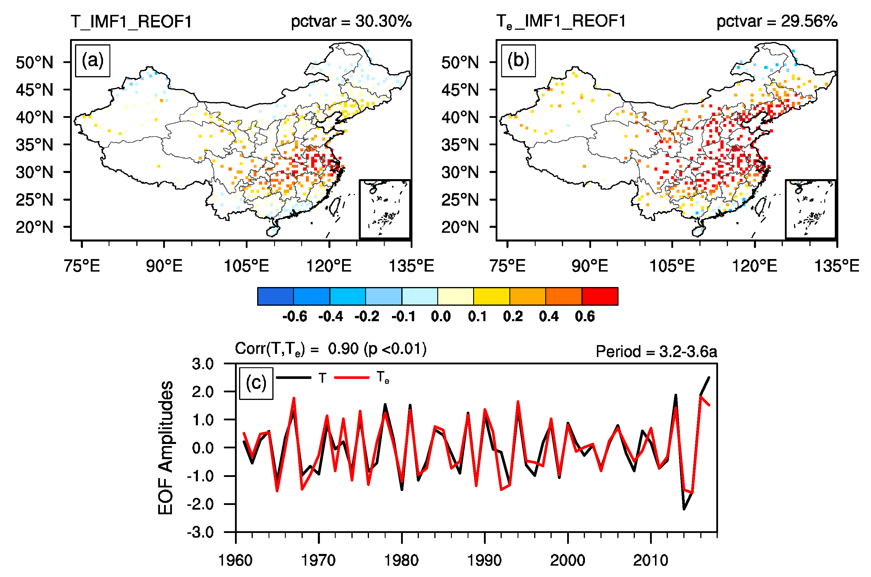
Specifically, the first REOF mode of the IMF 1 of T primarily shows a high-frequency time variation at the interannual scale (period of 3.2–3.6 years; Figure 2c), and the spatial pattern exhibits consistent changes throughout China (except for parts of South China and regions to the north of 45 °N in China; Figure 2a). Evident variations are detected in the Yangtze River basin, with an increase in T of more than 0.4 °C. For the first REOF mode of IMF 1 of T_e, the spatial feature of T_e also exhibits a consistent distribution pattern across the country, the PC of T and T_e are significantly positively correlated (the correlation coefficient is 0.90, p < 0.01). However, unlike the T distribution, where the large values are distributed solely in the Yangtze River basin, the large values of T_e are located in both the Yangtze River basin and most regions in northern China. In addition, the amplitude of change in T_e is significantly greater than that in T, specifically in northern China, where the amplitude of variation in T_e is approximately twice than that in T (Figure 2a vs. Figure 2b).

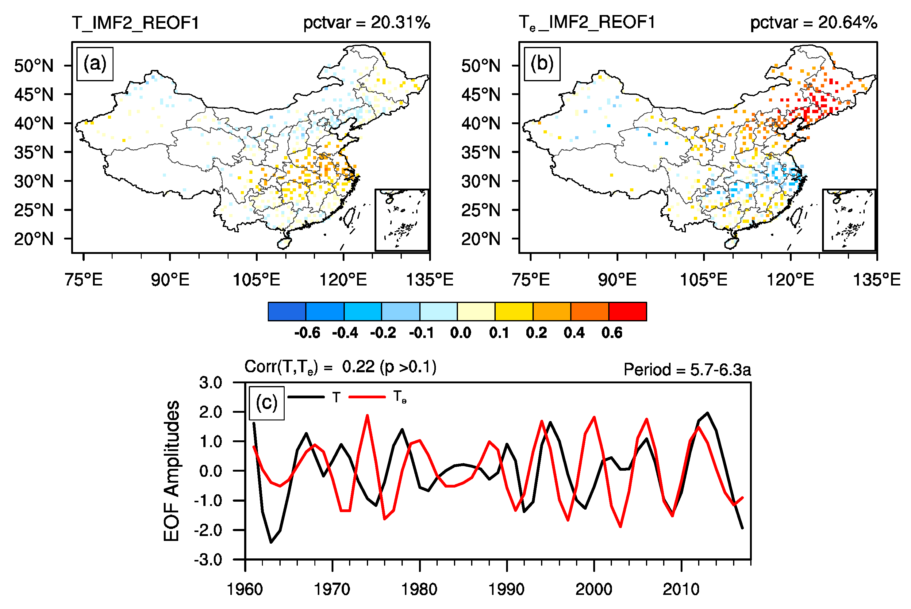
In the first REOF mode of IMF 2 of T with a quasi-6-year period (Figure 3c), the spatial pattern shows a “negative–positive” anti-phase relationship between northern and southern China, with a boundary of approximately 35° N, i.e., the temperature variations between southern and northern China are opposites (Figure 3a). The amplitude of the temperature variation of IMF 2 in the Yangtze-Huaihe region (approximately 0.4 °C) is significantly larger than that in the North China (smaller than −0.15 °C), which suggest that IMF 2 is probably dominated by the temperature variations in the quasi-6-year period in the Yangtze-Huaihe region. On the IMF 2 scale of T_e, in terms of both the spatial distribution and time series, there are considerable differences between T and T_e (Figure 3a vs. Figure 3b). Specifically, although T_e also exhibits opposite distributions in the south and north regions, the variations of T_e in northern China (especially in North China and Northeast China) are much stronger than that of T, and the largest warming amplitude is greater than 0.6 °C. Different from the IMF 2 leading mode of T that reflects the variations in the Yangtze-Huaihe region, the IMF 2 leading mode of T_e primarily reflects the significant anti-variations between the middle and low reaches of the Yangtze River (MLRYR) and northern China. In addition, there is no significant correlation between the time series corresponding to T and T_e (the correlation coefficient is only 0.22).

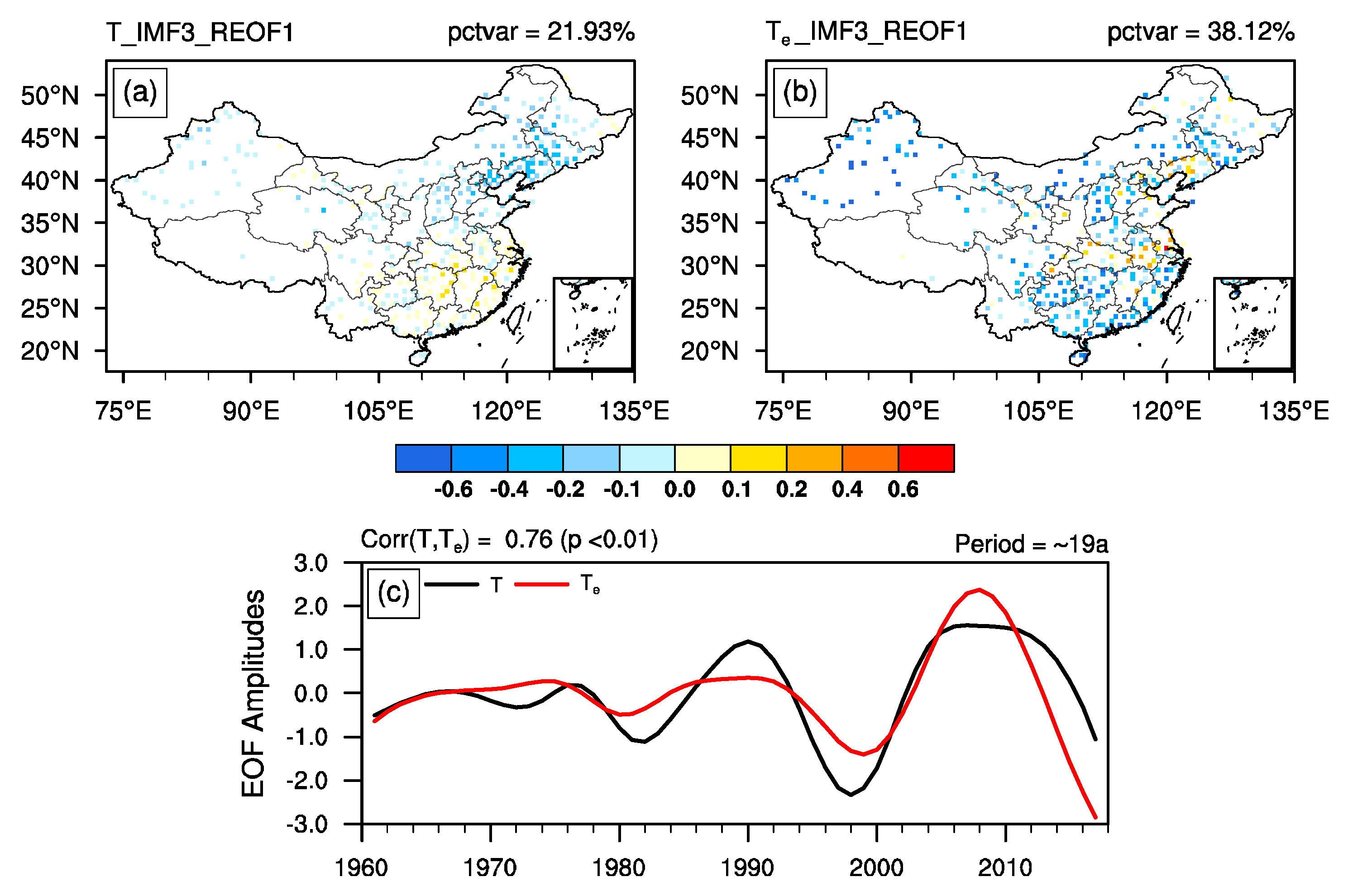
On the decadal scale (IMF 3 of a quasi-19-year period), the first REOF mode of IMF 3 of T also exhibits an anti-phase distribution in both northern and southern China (but with the Yangtze River as the boundary; Figure 4a). In contrast to IMF 2, the IMF 3′s REOF leading mode of T generally represents the variation in the Bohai Rim region (with the largest cooling of more than −0.6 °C), and the T variations in southern China are very slight (slight warming of no more than 0.2 °C). For T_e, although the correlation of the PCs corresponding to T and T_e is high (0.76, p < 0.01; Figure 4c), their spatial fields are distinguishable. In contrast to the spatial distribution of T exhibiting anti-variations in southern and northern China, the spatial feature of T_e exhibits cooling in most regions of China (except for slight warming occurs in some areas of MLRYR; Figure 4b), and the amplitude of T_e variation is significantly larger than that of T (more than −0.4 °C; Figure 4a vs. Figure 4b).

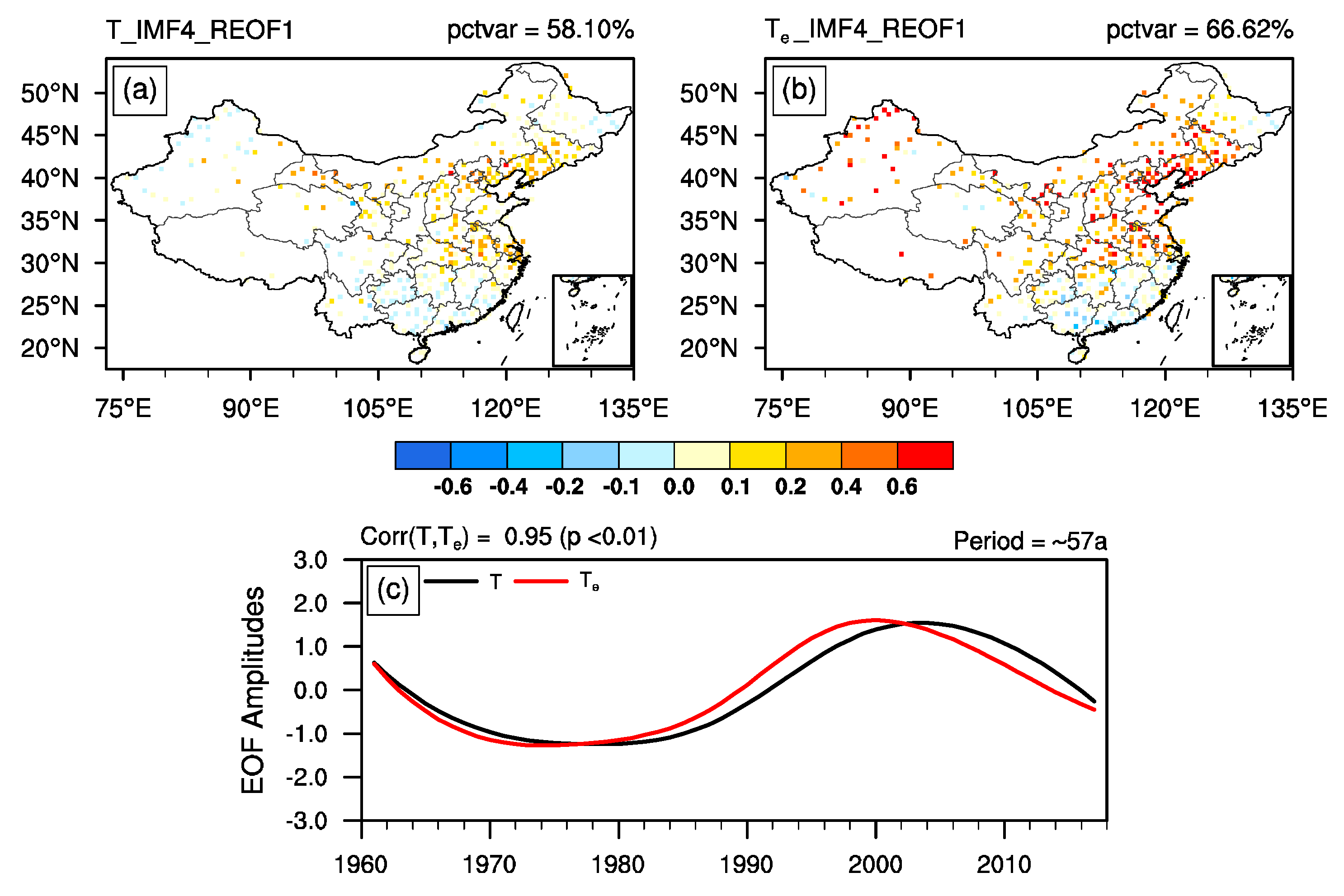
In the quasi-57-year cycle (IMF 4), overall, the variation in T is also generally consistent nationwide (Figure 5a); the large temperature variations primarily located in North China, the eastern part of Northwest China and East China (where the temperature increases approximately 0.3–0.4 °C). In other regions, the temperature variations of T are weak (approximately ± 0.15 °C; Figure 5a). Similar to the spatial distribution of T, T_e also shows consistent warming in most regions of China (Figure 5b), and their PCs are highly positively correlated (0.95, p < 0.01; Figure 5c). However, the primary difference between them is the amplitude of variations. In detail, the variation amplitude of T_e in North China, Northwest China and East China is significantly larger than that of T (Figure 5b).

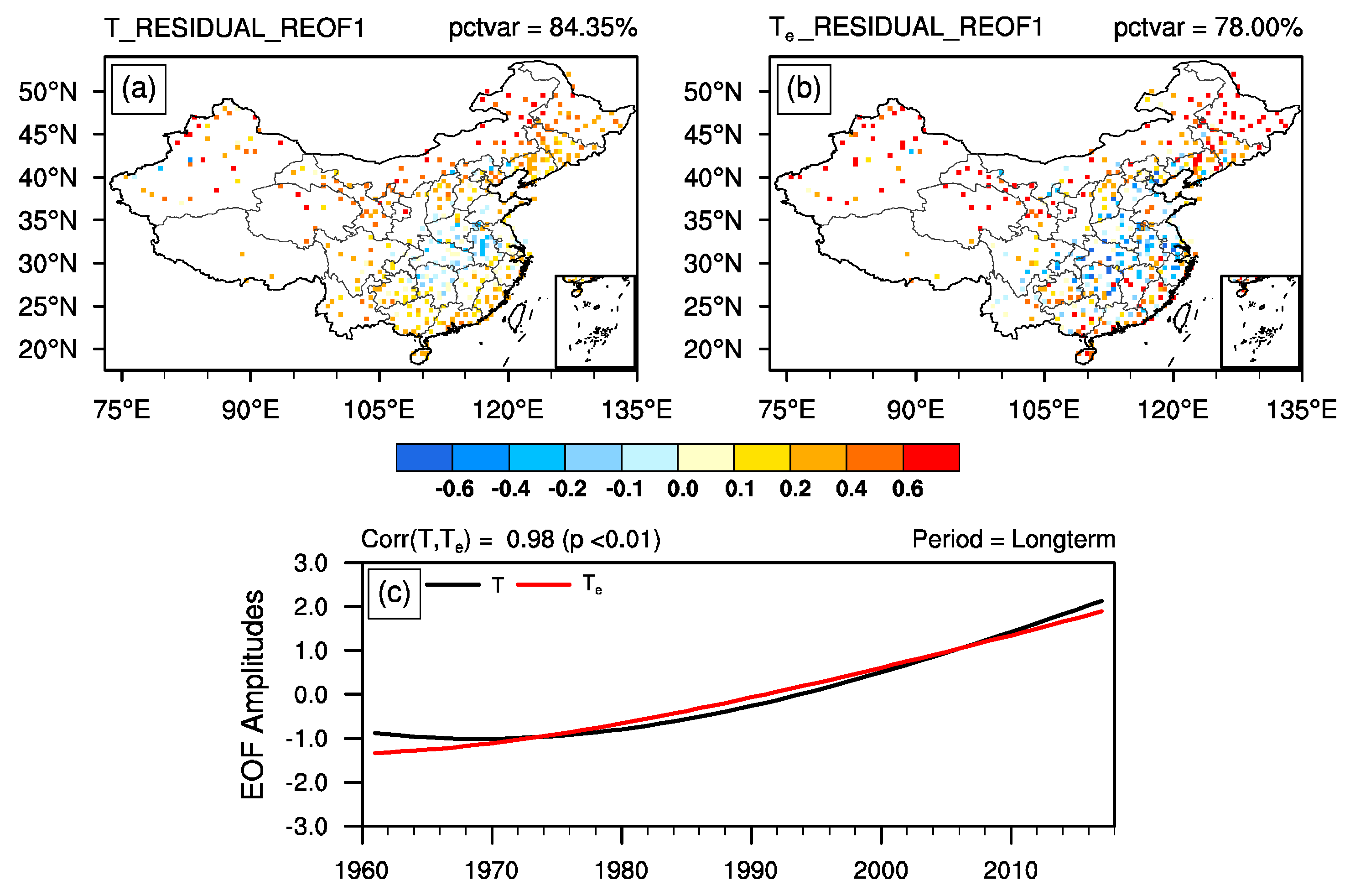
For the residual component (which exhibited a nonlinear trend), the temperature variation is dominated by warming in the northern region, and the amplitude of such warming is higher than 0.5 °C in most northern regions. In the southern region, the temperature variation is relatively weak, and there is a slight cooling in the Yangtze River basin, where the temperature variation is approximately within ± 0.2 °C (Figure 6a). Furthermore, T and T_e are consistent in that warming occurs in northern regions, and they are different in that the cooling is more prominent for T_e than for T in some southern regions (less than −0.4 °C in most regions; Figure 6b). It is noted that the REOF spatial–temporal variations of the residual mode are consistent with the warming trend in China during the recent decades [39].

In addition, based on the percent variances of all the leading mode of T and T_e at multiple timescales, REOF leading mode of both T and T_e at interannual scale (IMF 1), multidecadal scale (IMF 4) and especially the nonlinear trend scale (the residual component), can all well represent the actual temperature variation of the corresponding scale. In conclusion, similarities of T and T_e in both spatial and temporal variations are detected in three leading modes at IMF 1, IMF 4 and residual component scales, while differences between two temperatures (i.e., T and T_e) are detected in the other two scales (i.e., IMF 2 and IMF 3). It should be noted that although we have used a station redistribution algorithm to unify the station density in each grid, the inhomogeneity of the spatial distribution in still remains, which might introduce some uncertainties to the current results. For enhancing the confidence of the REOF results, we have tested the sensitivity of the EOF/REOF results to the station selection from the perspective of bootstrap resampling, details can be found in the supporting information (Text S1 and Figure S3). The results of random sampling show that the REOF1 spatial–temporal patterns at each timescale shown in our manuscript are generally not sensitive to the number and distribution of the stations.

3.2. The Role of T and LH Terms in Determining the Variations of T_e

In the previous section, we have comprehensively demonstrated the major differences between T and T_e at different timescales. The differences between these two temperatures theoretically suggest the role of introducing a latent heat term on the variations of T_e. Hence, in this section, further exploration and discussion will be conducted to show the relative role of T and LH terms in determining the variations of T_e.

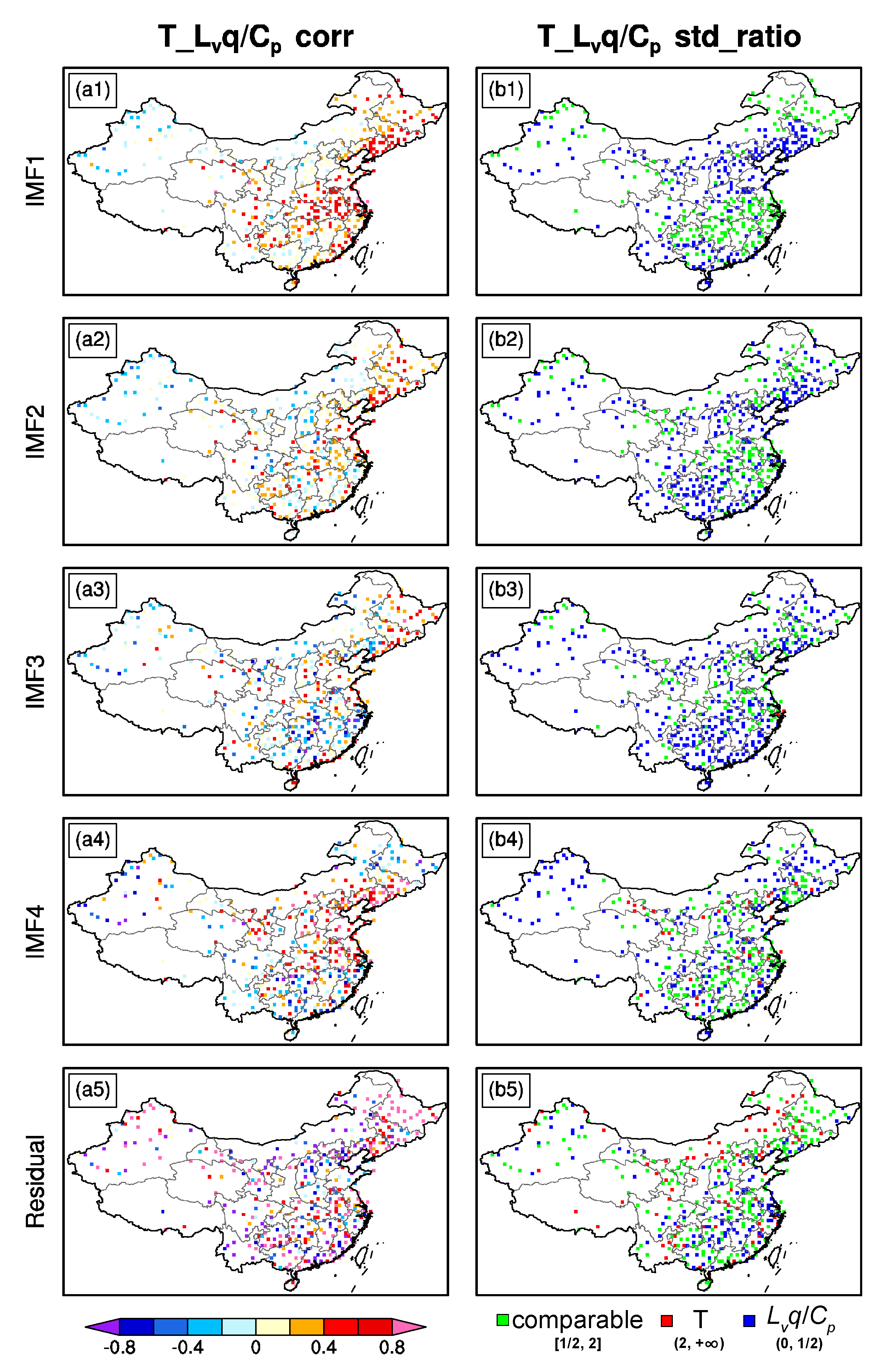
Generally, according to the formula of T_e, firstly, if the variations of T and T_e are similar, there are two possibilities: (1) The variability of T (V_T) is far greater than that of LH term (V_LH), i.e., V_T >> V_LH, which makes T_e dominating by T; and (2) V_T and V_LH are comparable or V_LH >> V_T, and the variations of T and LH term must be similar at the same time (i.e., the correlation between T and LH term are positive and high), which would result in the enhancement of T_e by the superposition effect of T and LH. Secondly, if the variations of T and T_e are distinguishable, then V_T and V_LH are comparable or V_LH >> V_T, and the variations between T and LH term should be negatively or lowly correlated. Thus, T_e would be dominated by the variation of LH and/or the joint variation of T and LH. In order to verify the above-mentioned conjectures and further our understanding of the possible causes of similarities and differences between T and T_e, we first additionally calculated the EEMD results of LH term (L_vq/C_p) to get the five EEMD modes of each grid. Furthermore, we calculate the correlation coefficients between EEMD-decomposed T and LH terms and the ratio of the standard deviations (STDR) between those two terms at different timescales. The correlation and STDR results are shown in Figure 7. Here, we define that STDR < 0.5, 0.5 ≤ STDR ≤ 2 and STDR > 2 represent that V_LH dominated the variability of T_e (V_Te), V_T and V_LH are comparable and T dominated V_Te, respectively.

In detail, for IMF 1, the correlations between T and LH terms exhibit high values (more than 0.6) over the Yangtze river basin ((a1) in Figure 7a), meanwhile, STDR between T and LH terms are comparable over the same region ((b1) in Figure 7b). However, the correlations of T and LH terms are weak in northern China (no more than ±0.2), and the STDR results in northern China indicate that V_LH is much larger than V_T. Those pieces of evidence suggest that the warming/cooling of T_e in northern China are dominated by V_LH, while T and LH probably increase or decrease simultaneously in the Yangtze River basin, which finally leads to a warm-humid or a cold-dry state in the summer climate of Yangtze River basin. For IMF 2, both the spatial and temporal results of REOF 1 are distinguishable between T and T_e (Figure 3). Unlike IMF 1, there is no evident correlation between V_T and V_LH (no more than ±0.4 over most of China; (a2) in Figure 7a), and the STDR results show that the anti-variation pattern in the REOF leading mode of T_e is probably influenced by the joint V_T-V_LH ((b2) in Figure 7b). Those results highlight that the variation of T_e is not a simple composition of T and LH, but can represent a unique complex nonlinear variation of coupled temperature-humidity. At the IMF 3 scale, the correlation pattern between T and LH resemble that of IMF 2, which also show sporadic correlations nationwide ((a3) in Figure 7a). From the STDR results of IMF 3, it is noted that V_LH is much greater than V_T over the regions with the strong variations of T_e (Figure 4b and (b3) in Figure 7b), which indicates that V_LH at the decadal scale is more important for surface heat content than V_T. For the multi-decadal scale (IMF 4), the REOF 1 spatial and temporal patterns between T and T_e are very similar, despite T_e with larger variations. The correlations between T and LH terms exhibit high values (more than 0.6) for regions with strong variations in both T and T_e (i.e., north of Yangtze River basin), which suggests that the multi-decadal variabilities of T and LH are similar ((a4) in Figure 7a). It is worth noting that STDR between T and LH terms in the previous three modes display either V_LH-dominated V_Te or a comparable situation, while at the multi-decadal timescale, V_T seems to be stronger than previous modes, specifically for some regions, dominant features of V_T are detected (i.e., some regions over MLRYR and northern China; (b4) in Figure 7b). Moreover, for the residual component, there are also high correlations (more than 0.6) all over the country, despite some evident negative correlations in North China ((a5) in Figure 7a). Interestingly, the role of V_T in determining V_Te further grows at the long-term trend scale from the STDR results. In detail, the STDR of T and LH show that V_T and V_LH are comparable over most of China, while V_T is much larger than V_LH in northern China, indicating that the nonlinear warming trend of T_e over northern China is dominated by V_T ((b5) in Figure 7b). In addition, from the REOF 1, correlations and STDR results of IMF 4 and the residual component, the relationships between T and LH on these two scales generally resemble that for IMF 1, i.e., the superposition effect of highly correlated T and LH (i.e., warm-humid or cold-dry) dominates the variation of T_e.

In addition, the above-mentioned results are completely consistent with our conjectures about the role of V_T and V_LH in determining the similarities and differences between T and T_e. In conclusion, V_LH plays an equivalent or more important role than V_T on V_Te at interannual to decadal scales (i.e., IMF 1–IMF 3), while V_T is being pronounced at multi-decadal and the long-term scales (i.e., IMF 4 and the residual component). These results also imply that the influencing factors and physical mechanisms leading to the changes in these two elements are likely to be different among timescales.

3.3. Similarities and Differences in the Linkage between SST and the Leading Mode of T and T_e

Previous studies have demonstrated that there is a close relationship between temperature variation in summer in China and SST variation in many key regions around the world (Pacific, North Atlantic and Indian Oceans) [24,25,40], especially on interdecadal and multidecadal scales (e.g., Wang et al. [41]). In the previous section, we have determined that except for the residual time series (which exhibits a nonlinear trend), the four main IMFs of T and T_e are interannual-to-multidecadal oscillations, and their similarities and differences are distinct at different timescales. Hence, what are the potential factors that cause a high correlation between the two temperatures (i.e., T and T_e) at the interannual, interdecadal and multidecadal scales (IMFs 1, 3 and 4)? What are the possible reasons for the low correlation between the two temperatures (i.e., T and T_e) at the interannual-to-interdecadal transition scale (IMF 2)? In this section, the possible linkage between the multi-timescale changes of the two temperatures (i.e., T and T_e) and the global SST is discussed. Note that we mainly focus on the first four IMF modes of T and T_e in this section; therefore, the detrending process is firstly done on the SST before calculating its correlation with the two temperatures.

Figure 8 presents the distribution of the correlation coefficients between the PCs of the first REOF modes of T and T_e and the SST in summer on each timescale, meanwhile,

Table 1. Correlation coefficients between summer SST indices and principal components of the first REOF mode of each IMF.

	EEMD-REOF Principal Components
SST Indices	T-IMF1	Te-IMF1	T-IMF2	Te-IMF2	T-IMF3	Te-IMF3	T-IMF4	Te-IMF4
Niño 3.4	−0.30 *	−0.43 *	0.06	−0.31 *	0.02	−0.11	−0.01	0.01
NAT	−0.03	−0.10	−0.03	−0.23	−0.03	−0.20	−0.37	−0.33
PDO	−0.17	−0.28	−0.04	−0.19	−0.13	−0.21	−0.08	0.05
AMO	0.06	0.12	0.01	0.09	0.17	0.01	0.67 *	0.59 *

* Asterisks in the table indicate that the correlation coefficients are statistically significant at 5% level.

lists the correlation coefficients between the PCs and multiple SST indices. In general, for the IMF 1 (Figure 8a,b) and IMF 4 scales (Figure 8g,h), the corresponding SST patterns that are significantly correlated with T resemble that with T_e, indicating that for these scales, the key SST patterns are associated with both V_T and V_LH. This also implies that the changes in SST in these key regions may not only affect the temperature variation in summer in China but also cause the coupled T-LH to increase or decrease simultaneously, i.e., warming (cooling) corresponds to high humidity (low humidity), which further causes the spatial distribution of T_e to be similar to that of T. However, in IMF 2 (Figure 7c,d) and IMF 3 (Figure 7e,f) modes, the corresponding SST patterns are different, indicating that the dominant key SST regions affecting T and T_e as well as the possible mechanisms are distinguishable for these two scales. This further suggests that for these two timescales, the differences in the corresponding SST patterns between T and T_e potentially highlight the possible relationship between SST and V_LH.

The SST fields associated with T and T_e of IMF 1 all exhibit significant reverse-phase changes in eastern and the western Pacific (i.e., positive and negative correlations over the western and eastern Pacific, respectively), which is obviously the typical El Niño–Southern Oscillation (ENSO)-type pattern (Figure 8a, 8b). The correlation coefficient between the PCs of T and T_e and the Niño 3.4 index is −0.30 (p < 0.05) and −0.43 (p < 0.05), respectively (Table 1), indicating that when the central and eastern equatorial Pacific SST is abnormally low in summer, T and T_e is high over the whole country. In addition, T and T_e are not only closely associated with ENSO-like SST anomalies (SSTA) in summer, but also positively correlated with the central and eastern equatorial Pacific SST in the preceding winter (Figure S4). This implies that the variations of T and T_e in summer may be modulated by the phase transition from El Nño (La Niña) in the preceding winter to La Niña (El Nño) in summer. Numerous studies have revealed that such transition, e.g., from El Nño to La Niña, typically results in a significant strengthening of the western Pacific subtropical high in summer, leading to clear skies (i.e., fewer clouds) with high temperatures in China (e.g., Wang et al. [42]). Moreover, it is noted that although the correlation coefficient patterns of T and T_e with SST is relatively consistent, T_e is detected to have a higher correlation with more significant signals than T. This indicates that the central and eastern equatorial Pacific SST not only affects the temperature but also causes the humidity to change at the same time, leading to the warm and wet (or cold and dry) climate in summer in China. In IMF 4, the SST field is positively correlated with T and T_e in the whole region of the North Atlantic (especially in the eastern part with significant positive correlations; Figure 8g,h). This correlation pattern is similar to the AMO. The correlation coefficient between the AMO index and T and T_e reached 0.67 (p < 0.05) and 0.59 (p < 0.05), respectively (Table 1), indicating that the variations of T and T_e are probably related to AMO in this mode. In addition, significant but sporadic correlations of T and T_e with SST are also detected in some regions of Indian and Pacific Oceans (Figure 8g,h).

On the remaining two scales that T and T_e are evidently different (see Figure 3 and Figure 4), their correlations with SST are also distinguishable (Figure 8c–f). In detail, at the IMF 2 scale, the SSTA that are significantly correlated with T manifest only as the low-latitude and mid-latitude dipole-type distributions in the North Atlantic (Figure 8c). But for T_e, it is shown that broadly significant positive correlations are detected in the central and eastern equatorial Pacific, the northeast Pacific and Indian Oceans, whereas the correlations over North Atlantic show an insignificant NAT pattern. The correlations of T and T_e with the SST indices are approximately consistent with the aforementioned spatial distribution (Table 1). These results also imply that although the relationship between T and the equatorial Pacific, North Pacific and Indian Oceans’ SSTs is relatively weak in the quasi-6-year period, the abnormal change in SST in these key regions may be an important factor for the variations of surface heat content. In addition, based on the SST signals from the preceding winter and spring (Figure S5), T is shown to correspond to the La Niña (El Niño) event, which has a weak development from the preceding winter to spring and decays to a non-significant signal during summer, whereas T_e corresponds to the La Niña (El Niño) event that continuously developed from the preceding winter into the current summer. This indicates that whether the development of ENSO events can be maintained into the current summer is a possible cause of the differences in T and T_e. From another perspective, continuously intensifying La Niña (El Niño) events may significantly affect the variation of humidity (precipitation) in summer in China, which in turn reflects in the variations of surface heat content. On the IMF 3 scale (Figure 8e,f), the T-related SST field does not feature a significantly correlated signal; however, the T_e-related SST field has negative correlations in the central, east and north equatorial Pacific Ocean, indicating that this type of SST is more closely related with V_LH. Furthermore, although the PCs of T and T_e have a high correlation, the corresponding SST patterns are inconsistent. This may be because the correlation between the PCs of T and T_e is relatively low before the 1990s (0.60 in the period 1961–1985, compared with 0.90 in the period 1986–2010).

Except for the above four modes, the PCs of the residual component of T and T_e are consistent with the trend of global warming (Figure 6c), and both correspond to the global-scale increase of SST (Figure S6). The change of the two temperatures is probably due to increased CO₂ concentrations caused by human activities [2].

4. Conclusions and Discussion

Based on the EEMD method and the observational data (i.e., surface air temperature, relative humidity, pressure and global SST), this study analyzed the similarities and differences of the surface air temperature (T) and equivalent temperature (T_e) defined by the ME in summer at multiple timescales for the period 1961–2017, and their relationship with global SST. The conclusions are as follows:

(1) The similarity between T and T_e is that both can be decomposed into five timescales: IMFs 1–4 (3.2–3.6-year period, quasi-6-year period, quasi-19-year period and quasi-57-year period, respectively) and a residual component (nonlinear trend). In terms of the results of all timescales, the variation of the leading modes (i.e., the first REOF modes) of T and T_e is dominated by the high-frequency interannual (3.2–3.6-year) and multidecadal (quasi-57-year) variations and the nonlinear warming trend. Moreover, except for the interannual-to-interdecadal transitional scale (quasi-6-year), there are significant positive correlations between the PCs of the first REOF modes of T and T_e.

(2) The differences between T and T_e can be mainly concluded as follows: Seen from all the REOF leading modes of T and T_e at multiple timescales, the magnitude of T_e variation is always greater than that of T, indicating that the variation of multi-variable-defined surface heat content is larger than that of single temperature-defined. For IMF 1, IMF 4 and the residual component scales, the REOF 1 spatial patterns are generally similar, except for the large discrepancies in the amplitude of between T and T_e variations. Further explorations suggest that V_T and V_LH are generally positively correlated and both changes of them tend to enhance the variability of surface heat content simultaneously, and in turn, leading to a warm-humid (or cold-dry) state in summer. However, at IMF 2 and IMF 3 scales, the differences between T and T_e are evident, not only in the amplitude of variability but in the spatial pattern as well. For IMF 2 scale, although V_T and V_LH are comparable, their correlations are relatively weak, which in turn exert a unique coupled effect on the surface heat content. For IMF 3 scale, V_LH are much larger than V_T, and there are low correlations between them, which ultimately make V_LH dominate the variation of the surface heat content (T_e).

(3) From the correlations of SST with T and T_e, similarities are also found in IMF 1, IMF 4 and the residual component scales, which both T and T_e show the ENSO phase transitions (e.g., El Niño phase to La Niña phase; IMF 1), AMO-like (IMF 4) and the global warming-like SSTA patterns (the residual component), respectively. In terms of quasi-6-year (IMF 2) and quasi-19-year periods (IMF 3), the SST fields associated with T and T_e are different: The ENSO events that developed during the preceding winter and persisted until summer for the quasi-6-year period possibly caused the difference between T and T_e. For the quasi-19-year period, the SSTA in the key regions of the central, east, and the north equatorial Pacific Ocean was closely related to T_e but not significantly correlated with T.

From the current results, this paper primarily emphasizes the similarities and differences of T and T_e at multiple timescales over China and shows some linkage between SST and T/T_e. Additionally, there are some limitations in this study, primarily in the following aspects. First, in terms of SST, this article only explored its relationship with T and T_e from the perspective of correlation, and the corresponding physical processes and mechanisms require further study. Second, in addition to the SST, there are many factors affecting T and T_e. For example, the results of Findell et al. [13] revealed that the land-use change in the historical period made parts of northern China significantly warmer and drier and made some parts of southern China warmer and more humid. The effects of other factors on T and T_e at different timescales require comprehensive investigation. Third, based on the main results of this paper, for the interannual-to-interdecadal scale (6 to 19-year period), there are very robust differences between T and T_e. The specific physical mechanism for the difference also deserves comprehensive discussion. In addition, we only show the results of the differences between T and T_e over China, however, the differences between T and T_e may be a global phenomenon (e.g., Li et al. [43]), since the reason for their differences is possibly due to the large-scale external forcings (e.g., anthropogenic greenhouse gases) or the internal variability (e.g., Rossby wave trains). Many other studies have also found that there are significant differences between T and T_e over other countries or globally (e.g., Pielke et al. [6], Younger et al. [17] and Li et al. [43]), and their differences at a multiscale over the rest of the world, as well as whether there is a potential linkage with our findings will require further investigations.

Despite these shortcomings, this article comprehensively discusses the characteristics of variations of T_e at multiple timescales in recent decades and their similarities and differences with those of T from a new perspective of joint temperature-humidity-defined surface heat content. The relevant results are intended to provide clues for the variations in the T_e-related total surface heat content and provide insights and bases for the comprehensive understanding of climate change as well as the related compound extreme events (e.g., compound temperature-humidity extremes) in recent decades.

References

1. IPCC. Climate Change 2007: The Physical Science Basis; Cambridge University Press: Cambridge, UK, 2007.
2. IPCC. Climate Change 2013: The Physical Science Basis; Cambridge University Press: Cambridge, UK, 2013.
3. IPCC. Climate Change 2018: Global Warming of 1.5°C. 2018; in press. Available online: https://www.ipcc.ch/sr15/ (accessed on 3 August 2019).
4. IPCC. Managing the Risks of Extreme Events and Disasters to Advance Climate Change Adaptation; Cambridge University Press: Cambridge, UK, 2012.
5. Qian, C.; Zhang, X.; Li, Z. Linear trends in temperature extremes in China, with an emphasis on non-Gaussian and serially dependent characteristics. Clim. Dyn. 2018, 53, 533–550. [Google Scholar] [CrossRef] [Green Version]
6. Pielke Sr, R.A.; Davey, C.; Morgan, J. Assessing “global warming” with surface heat content. Eos Trans. Am. Geophys. Union 2004, 85, 210–211. [Google Scholar] [CrossRef]
7. Davey, C.A.; Pielke, R.A.; Gallo, K.P. Differences between near-surface equivalent temperature and temperature trends for the Eastern United States: Equivalent temperature as an alternative measure of heat content. Glob. Planet. Chang. 2006, 54, 19–32. [Google Scholar] [CrossRef]
8. Fall, S.; Diffenbaugh, N.S.; Niyogi, D.; Pielke Sr, R.A.; Rochon, G. Temperature and equivalent temperature over the United States (1979–2005). Int. J. Climatol. 2010, 30, 2045–2054. [Google Scholar] [CrossRef]
9. Sherwood, S.C.; Huber, M. An adaptability limit to climate change due to heat stress. Proc. Natl. Acad. Sci. USA 2010, 107, 9552–9555. [Google Scholar] [CrossRef] [PubMed] [Green Version]
10. Dunne, J.P.; Stouffer, R.J.; John, J.G. Reductions in labour capacity from heat stress under climate warming. Nat. Clim. Chang. 2013, 3, 563–566. [Google Scholar] [CrossRef]
11. Knutson, T.R.; Ploshay, J.J. Detection of anthropogenic influence on a summertime heat stress index. Clim. Chang. 2016, 138, 25–39. [Google Scholar] [CrossRef] [Green Version]
12. Pal, J.S.; Eltahir, E.A.B. Future temperature in southwest Asia projected to exceed a threshold for human adaptability. Nat. Clim. Chang. 2016, 6, 197–200. [Google Scholar] [CrossRef]
13. Findell, K.L.; Berg, A.; Gentine, P.; Krasting, J.P.; Lintner, B.R.; Malyshev, S.; Santanello, J.A.; Shevliakova, E. The impact of anthropogenic land use and land cover change on regional climate extremes. Nat. Commun. 2017, 8, 989. [Google Scholar] [CrossRef] [PubMed]
14. Karl, T.R.; Knight, R.W. The 1995 Chicago heat wave: How likely is a recurrence? Bull. Am. Meteorol. Soc. 1997, 78, 1107–1120. [Google Scholar] [CrossRef]
15. Grumm, R.H. The central European and Russian heat event of July–August 2010. Bull. Am. Meteorol. Soc. 2011, 92, 1285–1296. [Google Scholar] [CrossRef]
16. Kang, S.; Eltahir, E.A.B. North china plain threatened by deadly heatwaves due to climate change and irrigation. Nat. Commun. 2018, 9, 2894. [Google Scholar] [CrossRef] [PubMed]
17. Younger, K.; Mahmood, R.; Goodrich, G.; Pielke, R.A.; Durkee, J. Mesoscale surface equivalent temperature (te) for east central USA. Theor. Appl. Climatol. 2019, 136, 65–75. [Google Scholar] [CrossRef]
18. Yin, H.; Sun, Y.; Wan, H.; Zhang, X.; Lu, C. Detection of anthropogenic influence on the intensity of extreme temperatures in China. Int. J. Climatol. 2017, 37, 1229–1237. [Google Scholar] [CrossRef]
19. Sun, Y.; Zhang, X.; Zwiers, F.W.; Song, L.; Wan, H.; Hu, T.; Yin, H.; Ren, G. Rapid increase in the risk of extreme summer heat in Eastern China. Nat. Clim. Chang. 2014, 4, 1082–1085. [Google Scholar] [CrossRef]
20. Qian, C. On trend estimation and significance testing for non-Gaussian and serially dependent data: Quantifying the urbanization effect on trends in hot extremes in the megacity of Shanghai. Clim. Dyn. 2016, 47, 329–344. [Google Scholar] [CrossRef]
21. Ren, G.; Zhou, Y. Urbanization effect on trends of extreme temperature indices of national stations over mainland China, 1961–2008. J. Clim. 2014, 27, 2340–2360. [Google Scholar] [CrossRef]
22. Qian, C.; Yan, Z.; Cao, L.; Li, Z. Climatic changes in the twenty-four solar terms based on temperature observations back to 1873. Clim. Environ. Res. 2018, 23, 670–682. (In Chinese) [Google Scholar] [CrossRef]
23. Wu, Z.; Jiang, Z.; Li, J.; Zhong, S.; Wang, L. Possible association of the western Tibetan Plateau snow cover with the decadal to interdecadal variations of northern China heatwave frequency. Clim. Dyn. 2012, 39, 2393–2402. [Google Scholar] [CrossRef]
24. Hu, K.; Huang, G.; Huang, R. The impact of tropical Indian Ocean variability on summer surface air temperature in China. J. Clim. 2011, 24, 5365–5377. [Google Scholar] [CrossRef]
25. Wu, R.; Yang, S.; Liu, S.; Sun, L.; Lian, Y.; Gao, Z. Changes in the relationship between Northeast China summer temperature and ENSO. J. Geophys. Res. Atmos. 2010, 115, D21107. [Google Scholar] [CrossRef]
26. Chen, Y.; Zhai, P. Revisiting summertime hot extremes in China during 1961–2015: Overlooked compound extremes and significant changes. Geophys. Res. Lett. 2017, 44, 5096–5103. [Google Scholar] [CrossRef]
27. Zhang, J.; Sun, F.; Xu, J.; Chen, Y.; Sang, Y.-F.; Liu, C. Dependence of trends in and sensitivity of drought over china (1961–2013) on potential evaporation model. Geophys. Res. Lett. 2016, 43, 206–213. [Google Scholar] [CrossRef]
28. Chai, R.; Sun, S.; Chen, H.; Zhou, S. Changes in reference evapotranspiration over china during 1960–2012: Attributions and relationships with atmospheric circulation. Hydrol. Process. 2018, 32, 3032–3048. [Google Scholar] [CrossRef]
29. Pielke Sr, R.A. Influence of the spatial distribution of vegetation and soils on the prediction of cumulus Convective rainfall. Rev. Geophys. 2001, 39, 151–177. [Google Scholar] [CrossRef]
30. Henderson-Sellers, B. A new formula for latent heat of vaporization of water as a function of temperature. Q. J. R. Meteorol. Soc. 1984, 110, 1186–1190. [Google Scholar] [CrossRef]
31. Wu, Z.; Huang, N.E. Ensemble empirical mode decomposition: A noise-assisted data analysis method. Adv. Adapt. Data Anal. 2009, 1, 1–41. [Google Scholar] [CrossRef]
32. Huang, N.E.; Shen, Z.; Long, S.R.; Wu, M.C.; Shih, H.H.; Zheng, Q.; Yen, N.-C.; Tung, C.C.; Liu, H.H. The empirical mode decomposition and the Hilbert spectrum for nonlinear and non-stationary time series analysis. Proc. R. Soc. Lond. Ser. A Math. Phys. Eng. Sci. 1998, 454, 903–995. [Google Scholar] [CrossRef]
33. Qian, C.; Fu, C.; Wu, Z.; Yan, Z. On the secular change of spring onset at Stockholm. Geophys. Res. Lett. 2009, 36, L12706. [Google Scholar] [CrossRef]
34. Franzke, C. Nonlinear trends, long-range dependence, and climate noise properties of surface temperature. J. Clim. 2012, 25, 4172–4183. [Google Scholar] [CrossRef]
35. Kim, T.; Shin, J.-Y.; Kim, S.; Heo, J.-H. Identification of relationships between climate indices and long-term precipitation in south korea using ensemble empirical mode decomposition. J. Hydrol. 2018, 557, 726–739. [Google Scholar] [CrossRef]
36. Wu, Z.; Huang Norden, E. A study of the characteristics of white noise using the empirical mode decomposition method. Proc. R. Soc. Lond. Ser. A Math. Phys. Eng. Sci. 2004, 460, 1597–1611. [Google Scholar] [CrossRef]
37. Wilks, D.S. Chapter 12—Principal component (eof) analysis. In International Geophysics; Wilks, D.S., Ed.; Academic Press: Cambridge, MA, USA, 2011; Volume 100, pp. 519–562. [Google Scholar]
38. Bretherton, C.S.; Widmann, M.; Dymnikov, V.P.; Wallace, J.M.; Bladé, I. The effective number of spatial degrees of freedom of a time-varying field. J. Clim. 1999, 12, 1990–2009. [Google Scholar] [CrossRef]
39. Committee of Chinese National Assessment Report on Climate Change. Third China’s National Assessment Report on Climate Change; China Science Press: Beijing, China, 2015. (In Chinese) [Google Scholar]
40. Wu, R.; Yang, S.; Liu, S.; Sun, L.; Lian, Y.; Gao, Z. Northeast China summer temperature and North Atlantic SST. J. Geophys. Res. Atmos. 2011, 116, D16116. [Google Scholar] [CrossRef]
41. Wang, J.; Yang, B.A.O.; Ljungqvist, F.C.; Zhao, Y.A.N. The relationship between the Atlantic Multidecadal Oscillation and temperature variability in China during the last millennium. J. Quat. Sci. 2013, 28, 653–658. [Google Scholar] [CrossRef]
42. Wang, B.; Wu, R.; Fu, X. Pacific–East Asian teleconnection: How does ENSO affect East Asian climate? J. Clim. 2000, 13, 1517–1536. [Google Scholar] [CrossRef]
43. Li, J.; Chen, Y.D.; Gan, T.Y.; Lau, N.-C. Elevated increases in human-perceived temperature under climate warming. Nat. Clim. Chang. 2018, 8, 43–47. [Google Scholar] [CrossRef]
Figure 1. Locations of the homogenized 412 meteorological stations (a) and 408 station-redistributed grid boxes (b) over China. Note that BR and MLRYR in (a) means Bohai Rim area (115–124° E; 36–43° N) and the middle and low reaches of the Yangtze River (102.5–123° E; 26.5–34.5° N), respectively. The two blue curves in the figure represent the Yellow River (north) and the Yangtze River (south), respectively.
Atmosphere 10 00447 g001
Figure 2. The first rotated empirical orthogonal function (REOF) modes of the intrinsic mode functions (IMF) 1 of summertime T (a) and Te (b) in China, and the corresponding principal component (c). Note that the “pctvar” in the figure means percent variance; “Corr” means correlation coefficient between T and Te; Black (Red) line represents the principal component of T (Te).
Atmosphere 10 00447 g002
Figure 3. The first REOF modes of the IMF 2 of summertime T (a) and Te (b) in China, and the corresponding principal component (c). Note that the “pctvar” in the figure means percent variance; “Corr” means correlation coefficient between T and Te; Black (Red) line represents the principal component of T (Te).
Atmosphere 10 00447 g003
Figure 4. The first REOF modes of the IMF 3 of summertime T (a) and Te (b) in China, and the corresponding principal component (c). Note that the “pctvar” in the figure means percent variance; “Corr” means correlation coefficient between T and Te; Black (Red) line represents the principal component of T (Te).
Atmosphere 10 00447 g004
Figure 5. The first REOF modes of the IMF 4 of summertime T (a) and Te (b) in China, and the corresponding principal component (c). Note that the “pctvar” in the figure means percent variance; “Corr” means correlation coefficient between T and Te; Black (Red) line represents the principal component of T (Te).
Atmosphere 10 00447 g005
Figure 6. The first REOF modes of the residual component of summertime T (a) and Te (b) in China, and the corresponding principal component (c). Note that the “pctvar” in the figure means percent variance; “Corr” means correlation coefficient between T and Te; Black (Red) line represents the principal component of T (Te).
Atmosphere 10 00447 g006
Figure 7. The correlation coefficients between T and LH terms (left column: (a)), and the ratio of the standard deviations (STDR) of T and LH (right column: (b)) at different ensemble empirical mode decomposition (EEMD) modes (rows 1–5). Note that the green, red and blue points in column b represent that the variability of T and the variability of LH are comparable (0.5 ≤ STDR ≤ 2), the variability of T dominated the variability of Te (STDR > 2) and the variability of LH dominated the variability of Te (STDR < 0.5), respectively.
Atmosphere 10 00447 g007
Figure 8. The spatial distributions of correlation coefficients between summer sea surface temperatures (SSTs) and the principal components of the first REOF mode of the IMFs (Left panel: T; Right panel: Te). (a,b) IMF 1; (c,d) IMF 2, (e,f) IMF 3, (g,h) IMF 4. Black dots represent the correlation coefficients that are statistically significant at 5% level.
Atmosphere 10 00447 g008