5.3. Multi-Objective Model Setup
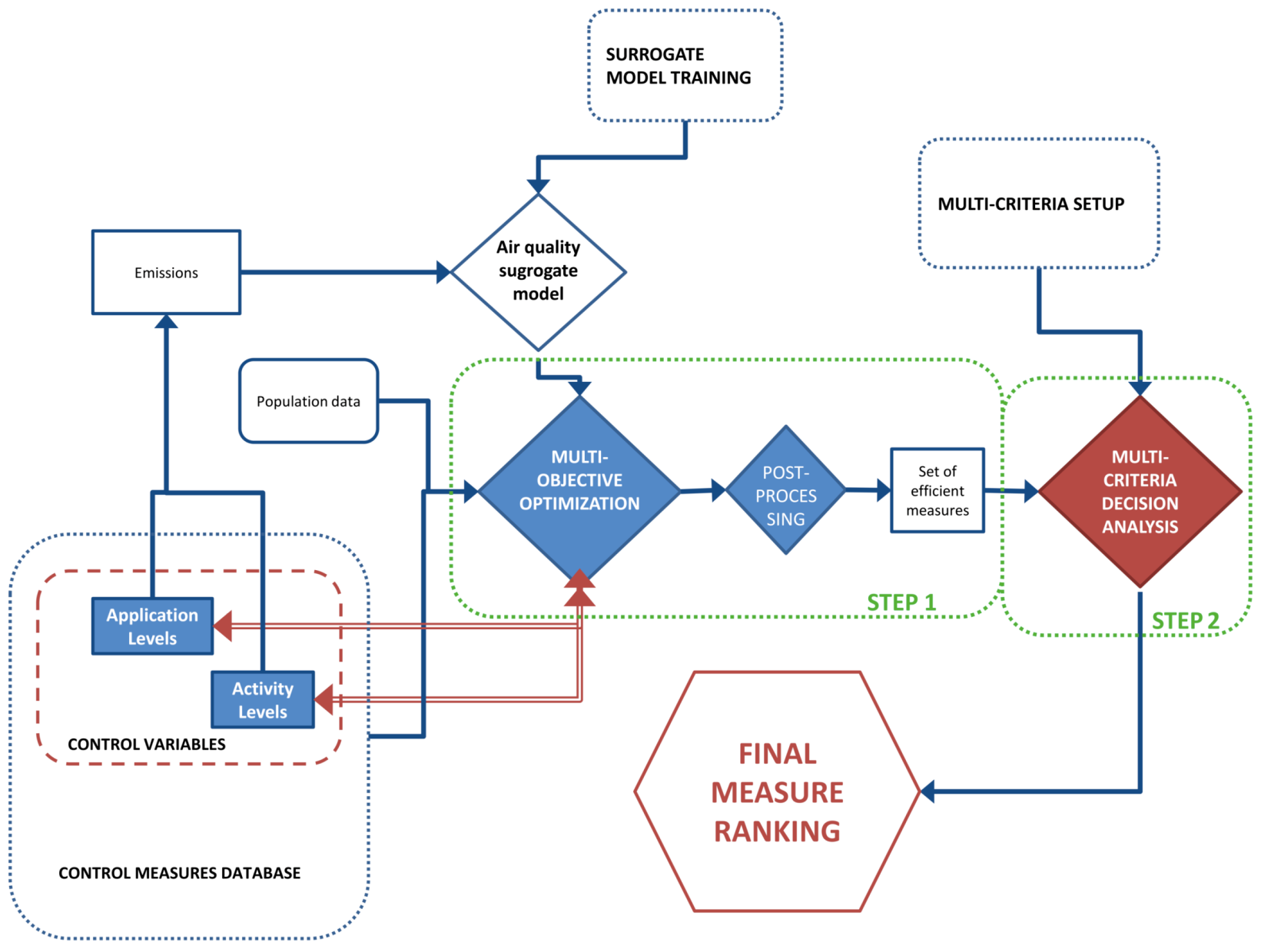
In the first step, since multiphase deterministic 3D modelling systems ([
29,
30]) cannot be used to compute pollutant concentrations and air quality indexes, due to the required computational cost and the number of simulations needed to solve a multi-objective problem, they have been substituted by statistical surrogate models, identified processing the results of a set of Chemical Transport Models simulations ([
31,
32,
33]). In particular, following the methodologies presented in [
34,
35,
36], models based on Artificial Neural Networks (ANNs), have been applied, mainly due to their features of low computational requirements, good performances and ability to reproduce non-linear functions. According to the same studies, three important features must be selected to identify a model that is adequate to the domain under study: radius of influence, input shape, and training data design. The first feature should be chosen considering that AQI values in a cell depend on precursor emissions generated in distant cells. While the second one allows to consider the dominant winds of the domain (mainly East-West and North-South in the current domain). Reference [
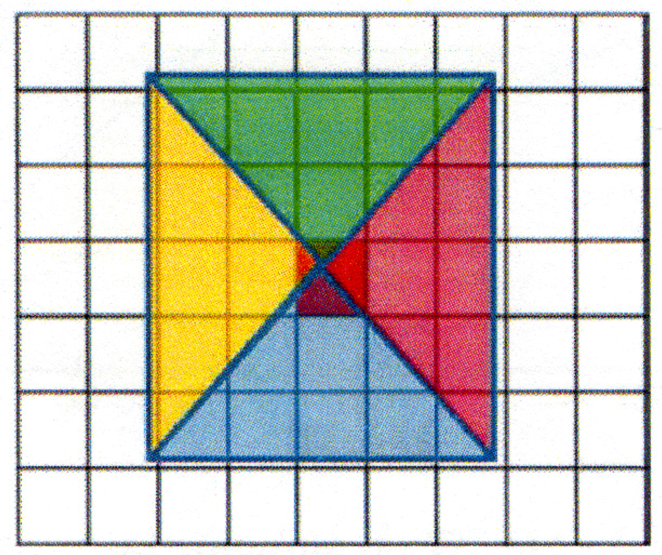
35] presented a technique allowing to consider both this aspect by summing the emissions of cells belonging to triangular slices around a target cell for which the model should be able to compute the AQI. An example of this scheme can be seen in
Appendix B—
Figure A1. Before the training of the models, also the extension of these slices (radius of influence) must be chosen so that it is appropriate for the AQI and the considered domain. To select the best radius of influence, different ANN models are identified by varying the radiuses. The radius choice falls on the ANN model showing the highest correlation and lowest mean squared error with respect to deterministic model simulations. The features of the Artificial Neural Network applied in the current work are summarized in
Table 1.
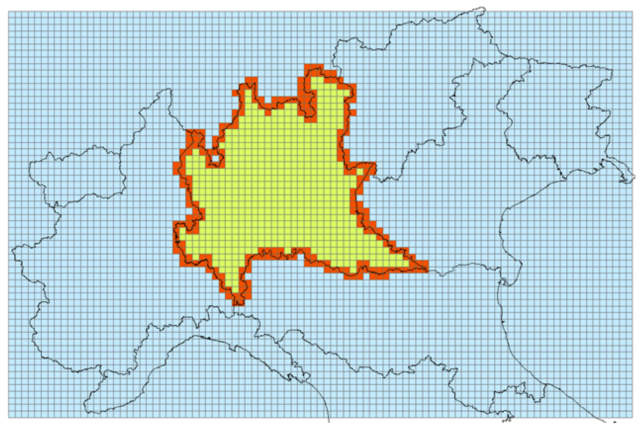
The set of scenarios needed to properly tune the surrogate model, has to be simulated by means of a deterministic model and should have the highest data variability in the input-output space (highest information content) and cover the possible emission variations of the precursors, but at the same time, the number of scenarios considered should be limited, due to the computational time required by the deterministic model. When applied in the Multi-objective problem, the surrogate model should reproduce scenarios in which the emissions of each precursor can vary between a maximum value, which corresponds to the maximum projected emissions for a chosen reference or “basecase” year, and a minimum value, representing the Maximum Feasible Reduction (MFR).
For this purpose two dummy extreme scenarios (HIGH and LOW scenario) can be defined by combining the maximum and the minimum values obtained from other 4 scenarios derived from the application of INEMAR 2008 emission inventory [
37] rescaled to 2010 and projection parameters derived from GAINS Italy database [
3].
Between the two extremes, a small number of emission scenarios are created by applying a Sobol sequences based algorithm [
38] in order to evenly distribute precursors emission values between the higher and lower possible values.
In
Appendix B—
Table A2 the precursor reduction factors derived from the algorithm are presented for each of the 14 emission scenarios that will be simulated and used for the surrogate model training.
These scenarios have been simulated by means of TCAM (Transport Chemical Aerosol Model), a three-dimensional Eulerian model [
39], in order to obtain the corresponding concentration scenarios needed for the training phase. These data are then divided into 2 smaller sets: one is the identification dataset used for the model training, containing 4/5 of the total data and the validation dataset, containing the remaining 1/5, used to evaluate the performances of the model. To perform this separation, all the training scenarios have been concatenated and 1 tuple every five has been extracted from the identification dataset and stored in the validation dataset.
Table 2 presents correlation (corr) and normalized root mean squared error (nrmse) for the validation dataset comparing TCAM target outputs and the ANN outputs. The first line refers to a comparison of the resulting concentrations, the second line shows the same indexes but computed on the concentration reductions with respect to the HIGH scenario in order to remove the effect of the background concentrations from the evaluation. High values of correlation (corr) and a low normalized root mean squared error (nrmse) attest the fitness of the model.
5.4. Results
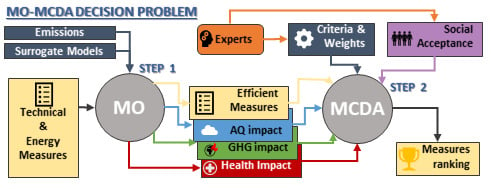
In the first part of this section, Step 1 results are shown and discussed. The objective of this stage is to find a small set of effective measures to be included in Step 2 and, also, to quantitatively evaluate through the system the performance that these measures have for some of the criteria that will be evaluated in the MCDA. The set of measures that has been evaluated through this first phase is composed of 288 end-of-pipe measures, 42 energy measures and 13 switch measures.
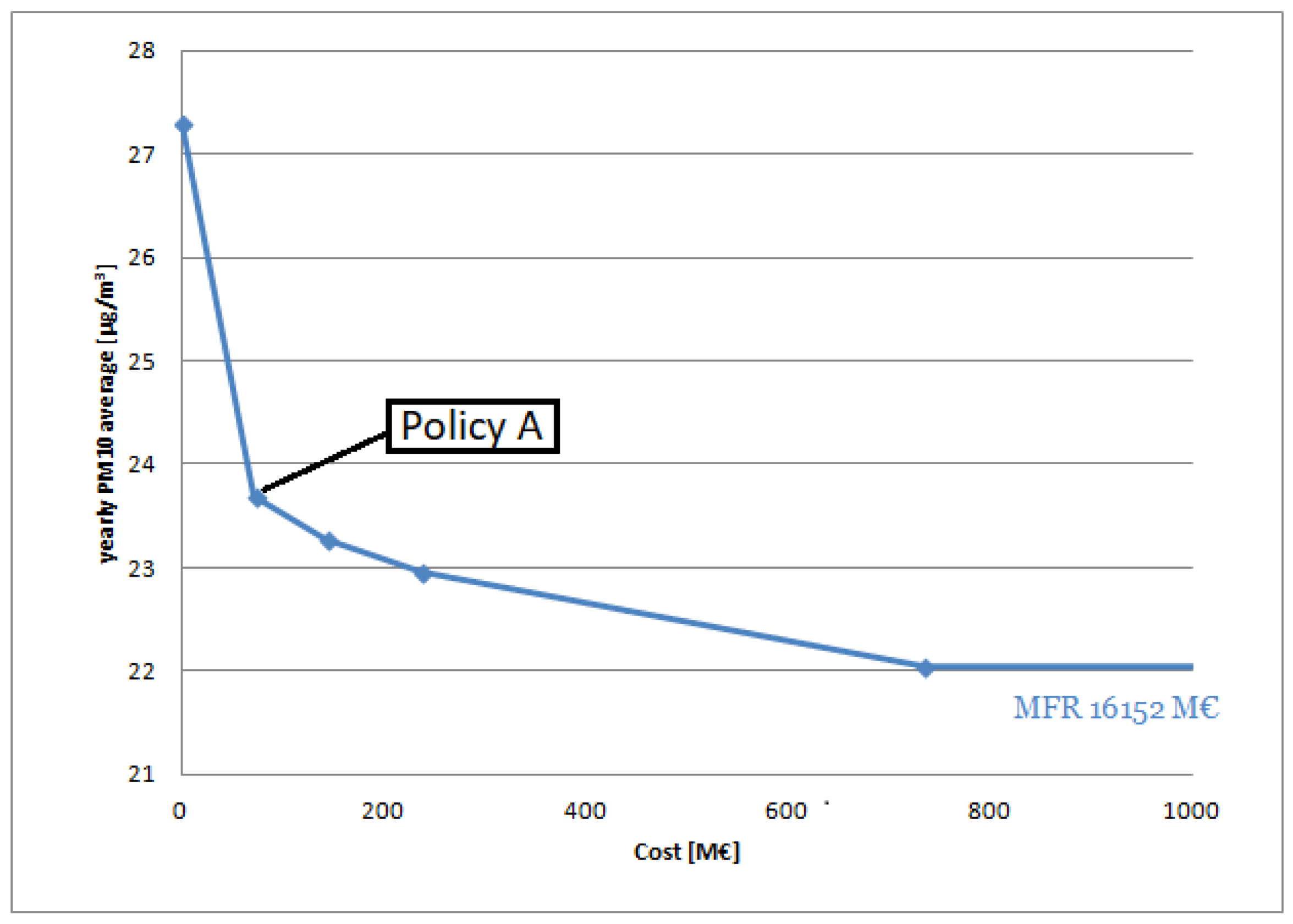
In
Figure 3, the Pareto front is shown, representing the solutions of the multi-objective problems in terms of cost and yearly average
concentrations. The starting scenario at the extreme left is the Current Legislation scenario expected for 2020, while the point on extreme right is the maximum feasible reduction obtainable with the considered measures while optimizing only the Air Quality objective. Due to the extremely high costs of some energy measures, the MFR has a cost of 16,152 M and a yearly average
concentration of 21.92
g/m
. This means that, by applying the policy identified by the the second point of the curve (72 M, 23.7
g/m
),
yearly average concentrations can be reduced of 67% with respect to the MFR at only the 0.3% of its cost.
In
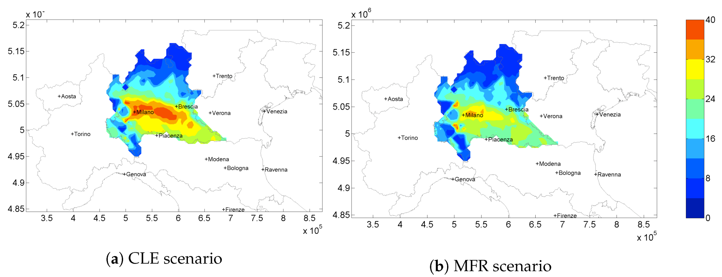
Figure 4 the
yearly average concentration maps for CLE 2020 scenario (
Figure 4a) and the Maximum Feasible Reduction obtainable (
Figure 4b) are shown.
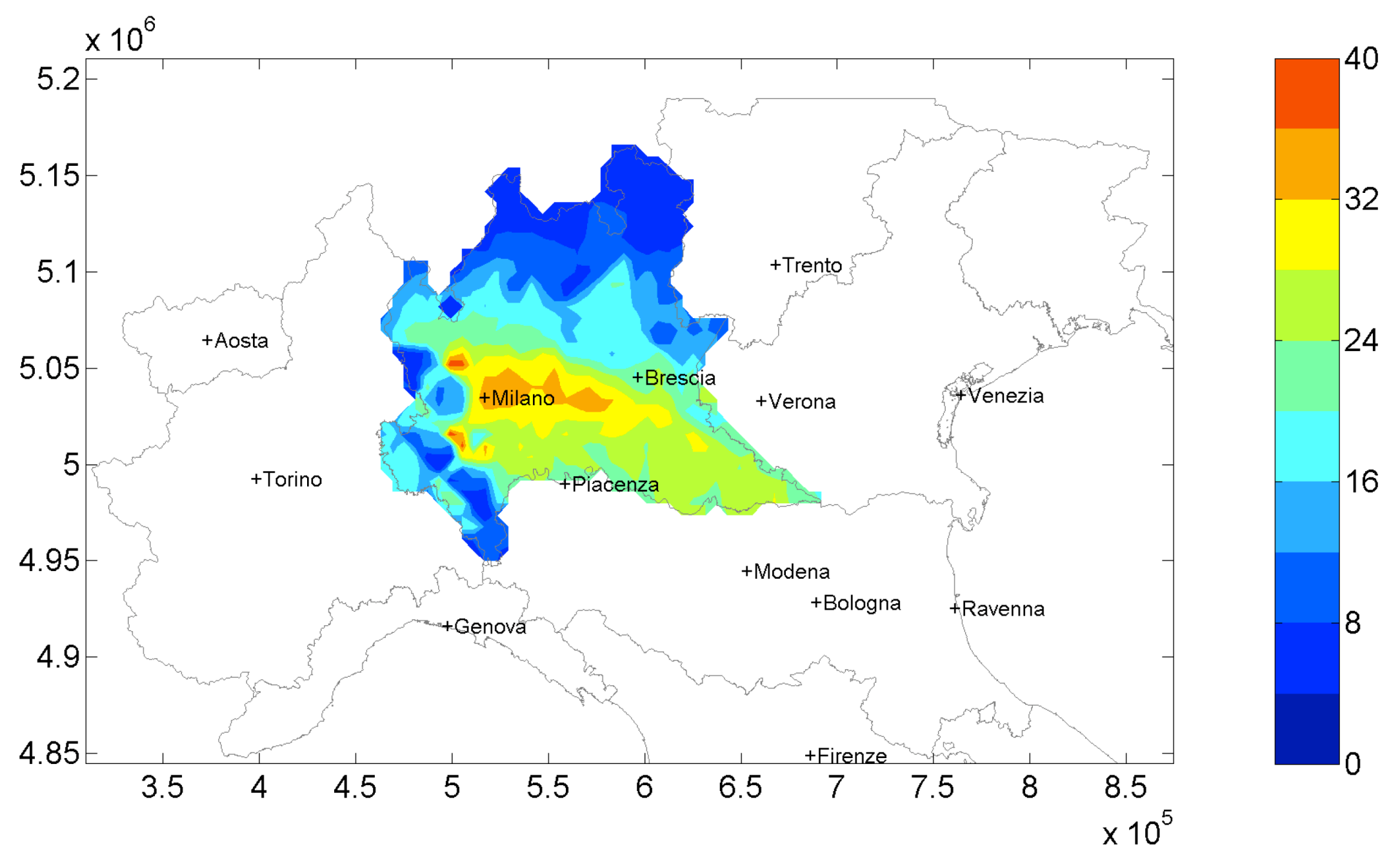
The same air quality index is shown in
Figure 5 for the solution at a 72 M/year cost (Policy A). This solution is one of the closest solution to the maximum curvature of the Pareto front. This means that a cost increase, with respect to this point, results only in a small decrease of
concentrations. The comparison between this last map with the maximum reduction obtainable (
Figure 4b), highlights that yearly
concentrations are not so different, except for small differences in the central part of the domain. So, adopting an effective solution such as Policy A, high amounts of
can be reduced over the domain at a low cost.
The yearly
concentrations obtained from Policy A show the effect of the combined application of nearly 100 measures whose application rates undergo an increase with respect to CLE scenario (starting point for the optimization). So, given also the impact of the non-linearities, it is not possible to define a-priori the set of measures with the highest impact on the AQI. The selected measures are the 10 measures with the highest
for energy and both end-of-pipe measures. In
Appendix C—
Table A3 the measures selected to undergo Step 2 are shown with their relative
values. Only 4 of the 13 energy measures are present in the table. The reason is that these measures are usually expensive, so, for a relatively low cost policy such as Policy A, only 4 of these are cheap enough to produce relevant effects on the air quality if little money is invested in them.
Once the measures have been selected, the MCDA can be applied, considering four criteria:
c1: social acceptance;
c2: implementation cost;
c3: health impact, in terms of YOLL due to long-term exposure;
c4: effect on GHGs emissions, considering equivalents.
All these criteria have scores ranged from 0 to 10 with an ascending direction of preference for all the criteria. This means that if a measure is the cheapest, it has the maximum score (10) in the cost criterion. Criterion c1, as well as the weighting factors for all the criteria, have been evaluated though a questionnaire submitted to a pool of experts. Instead, for the last three criteria (c2, c3 and c4), since it is possible to obtain reliable quantitative information by solving the multi-objective optimization, the scores attributed to each measure have been computed by applying the MOA individually to the selected measures. The values used for criteria c2, c3 and c4, are respectively computed through Equations (
3), (
6) and (
5). These data have then been normalized between 0 and 10 and the results are shown in
Table A4.
Appendix D—
Table A4 summarizes the performance coefficients and criteria weights chosen by the experts’ (performance matrix).
Preference thresholds are associated with the total number of alternatives to efficiently discriminate among the options, providing a smoothed “relative distance” between the alternatives. In order to achieve this, indifference and preference thresholds are computed for the different criteria (shown in
Appendix D—
Table A5) with the use of Equations (
8) and (9). Fixed thresholds were applied and veto thresholds were not considered. The methodological approach continues with the application of the LAMSADE ELECTRE III-IV package [
40] applying an outranking relation based on decision maker’s preferences and providing two partial pre-orders of alternatives: an ascending and a descending one.
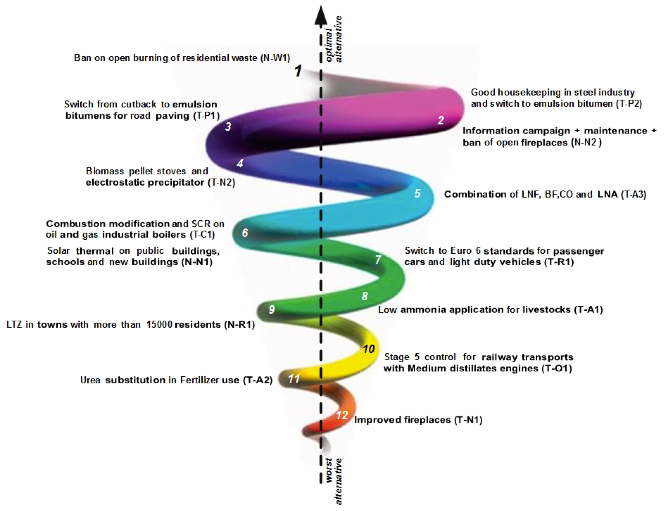
The merge of these two pre-orders is used to compute the final ranking of all alternatives, shown in
Figure 6. This figure presents the Median Pre-order, that is a complete pre-order and it is built in the following way: the alternatives are classified through an intersection of the distillations results and two incomparable alternatives in the same position are classified according to the differences in their positions in the two distillations. The first letter in the code identifies if a measure is end-of-pipe (T) or a fuel consumption measure (N).
The first measures in this ranking are: (1) “Ban on open burning of residential waste”, (2) “Good housekeeping in steel industry and switch to emulsion bitumen”, (3) “Information campaign + maintenance + ban of open fireplaces”. “Ban on open burning of residential waste” has high scores in the first two criteria, this means that it is considered socially acceptable and has a low cost. The health impact and effect on GHG emission scores are low but the experts assigned the lowest weights to these criteria. This is true also for measure T-P2, while the third measure has lower values in c1 and c2, but higher scores for health impact and effect on GHG emissions. It is possible to see that, despite the fact that only 4 energy measures were considered, two out of the three best measures are energy ones. The other two ranked 6th (N-N1) and 9th (N-R1) because of an extremely high cost (the first) and low scores in all the criteria except the cost (the second).
The multi criteria decision analysis approach is strongly dependent from the choice of the criteria to be considered and the experts’ views on criteria weights. In
Table 3, an example of the final measure ranking is shown, if the decision makers decide to ignore one of the criteria. The central column represent the ranking considering all the criteria, the left column shows the rank changes when leaving out the effect on GHG emissions, while the last one on the right presents the ranking when leaving out the effect on health. It can be seen that, due to the fact that the criteria removed are the ones with the lowest weight, even if there are small changes, the measures in the first places are the same, despite few position changes. The same happens for the last positions. This dependence on subjective choices stresses the need of a consider a shared choice of the criteria among the people involved in the decision process and a wide pool of stakeholders to evaluate the measure scores for the different criteria when modelling data are not available.
