Estimation of Sensible Heat Flux and Atmospheric Boundary Layer Height Using an Unmanned Aerial Vehicle


Abstract
1. Introduction
2. Methods
2.1. Bulk Method
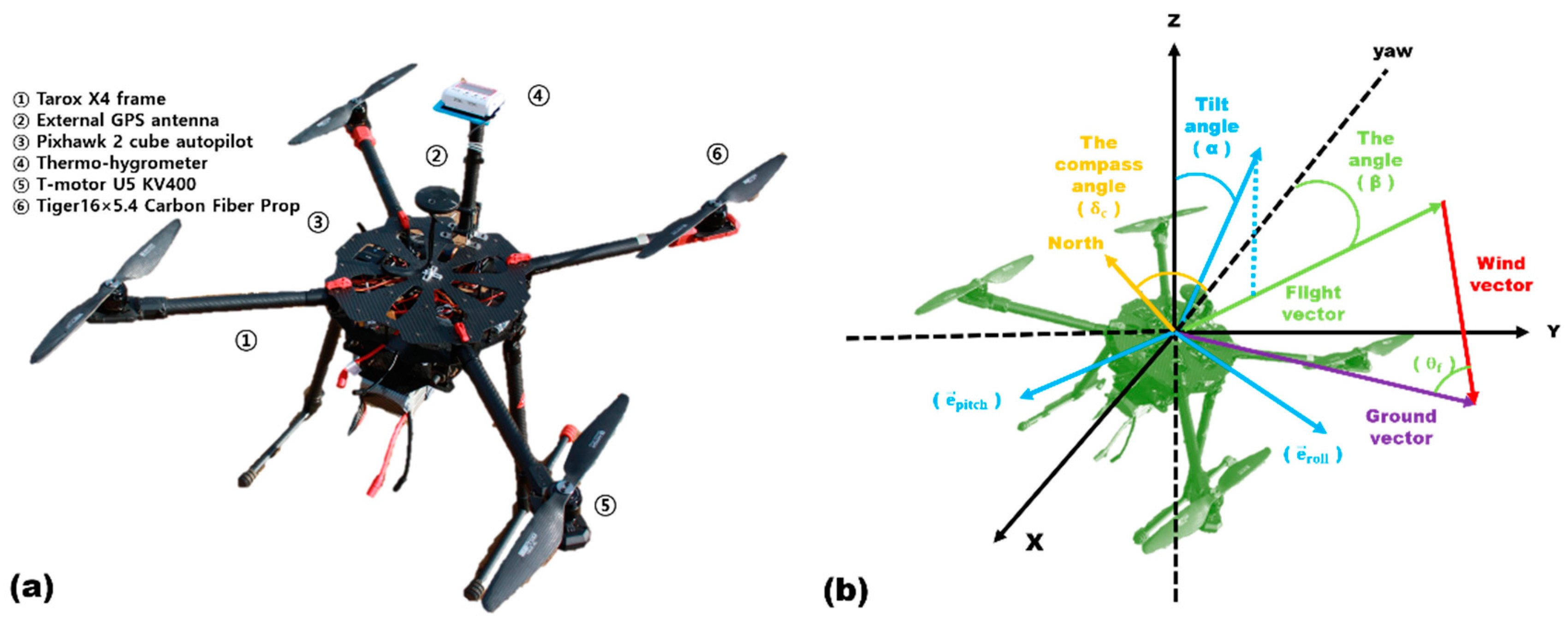
2.2. Unmanned-Aerial-Vehicle-Based Wind Speed
3. Results and Discussion
3.1. Sensible Heat Flux
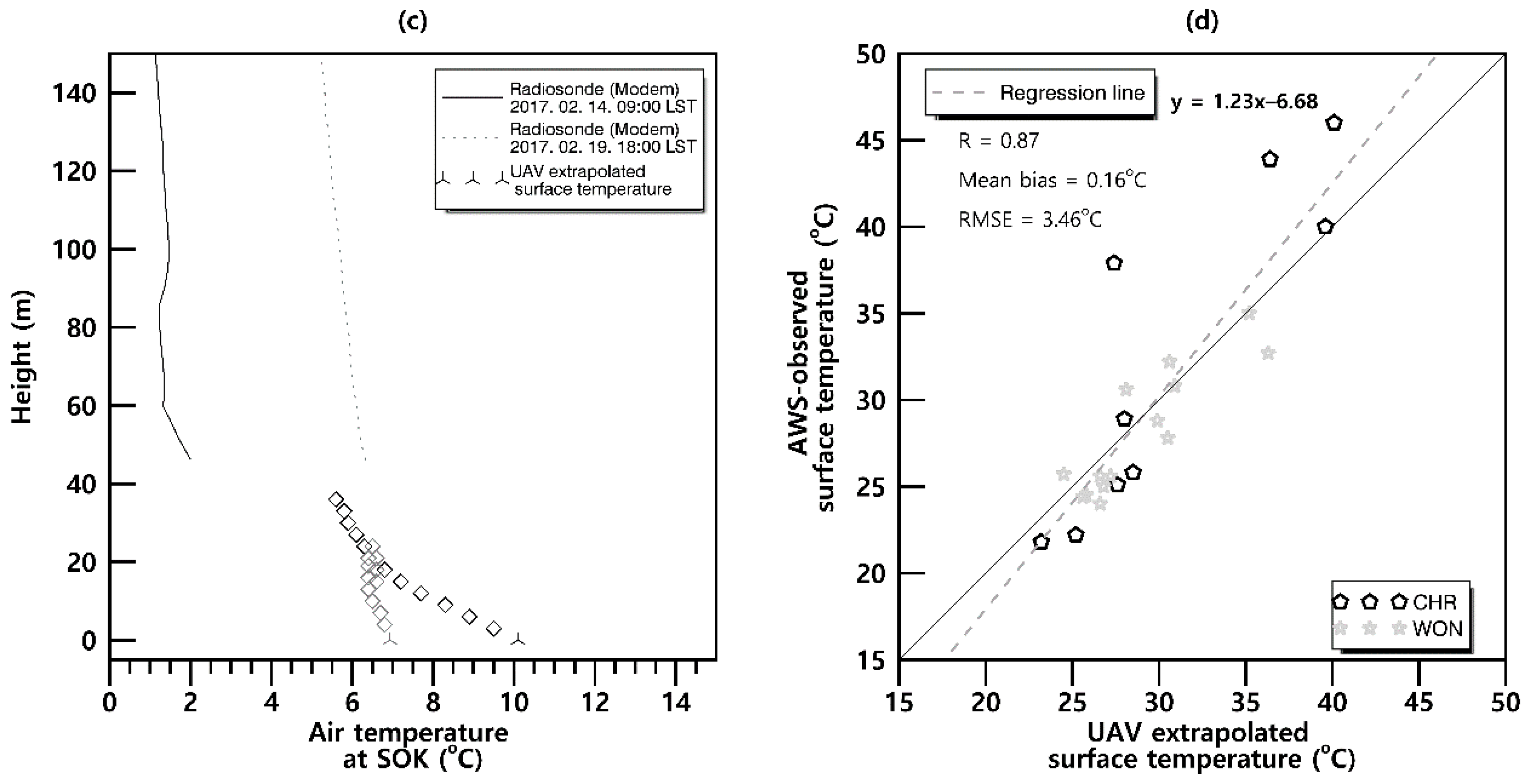
3.2. Temperature and Wind Speed from Rotary-Wing UAV
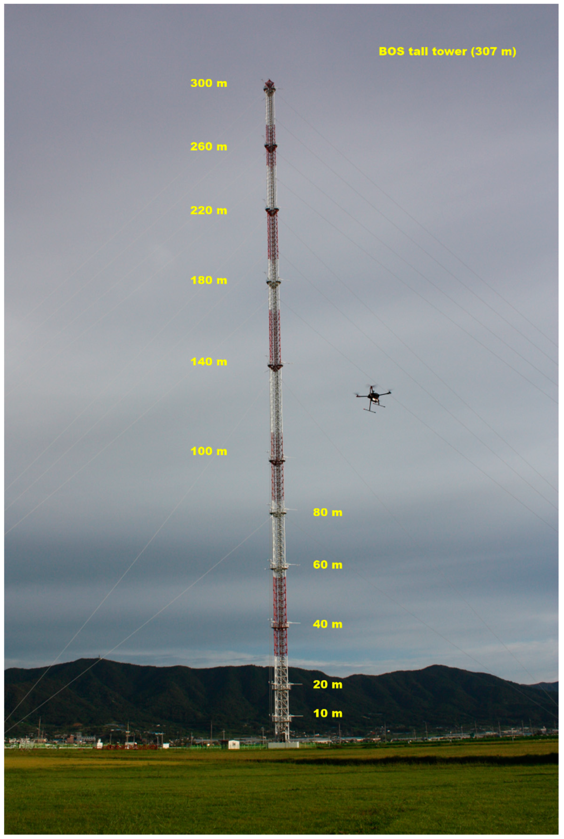
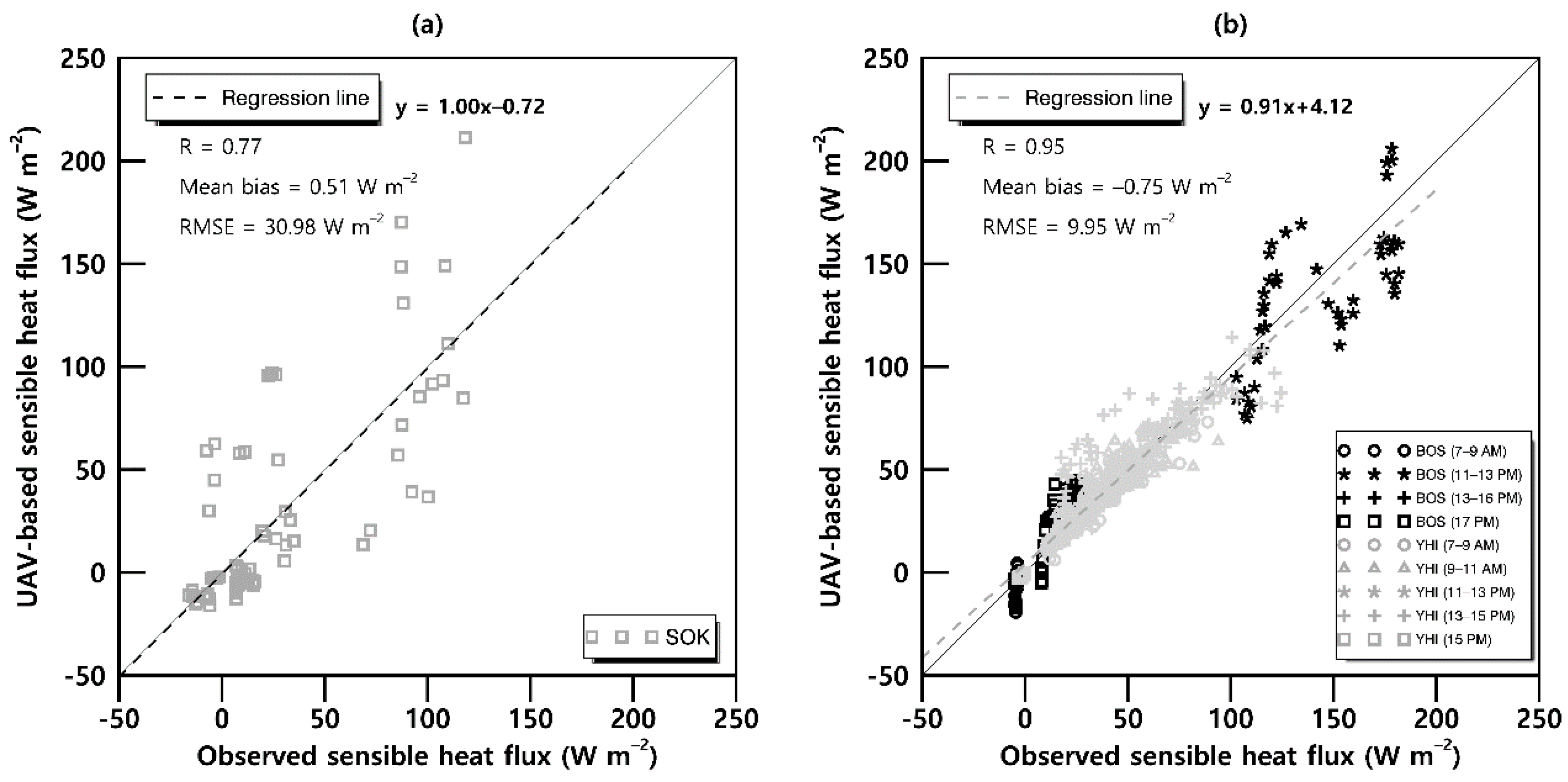
3.3. Heat Flux Based on Rotary-Wing UAV Hovering
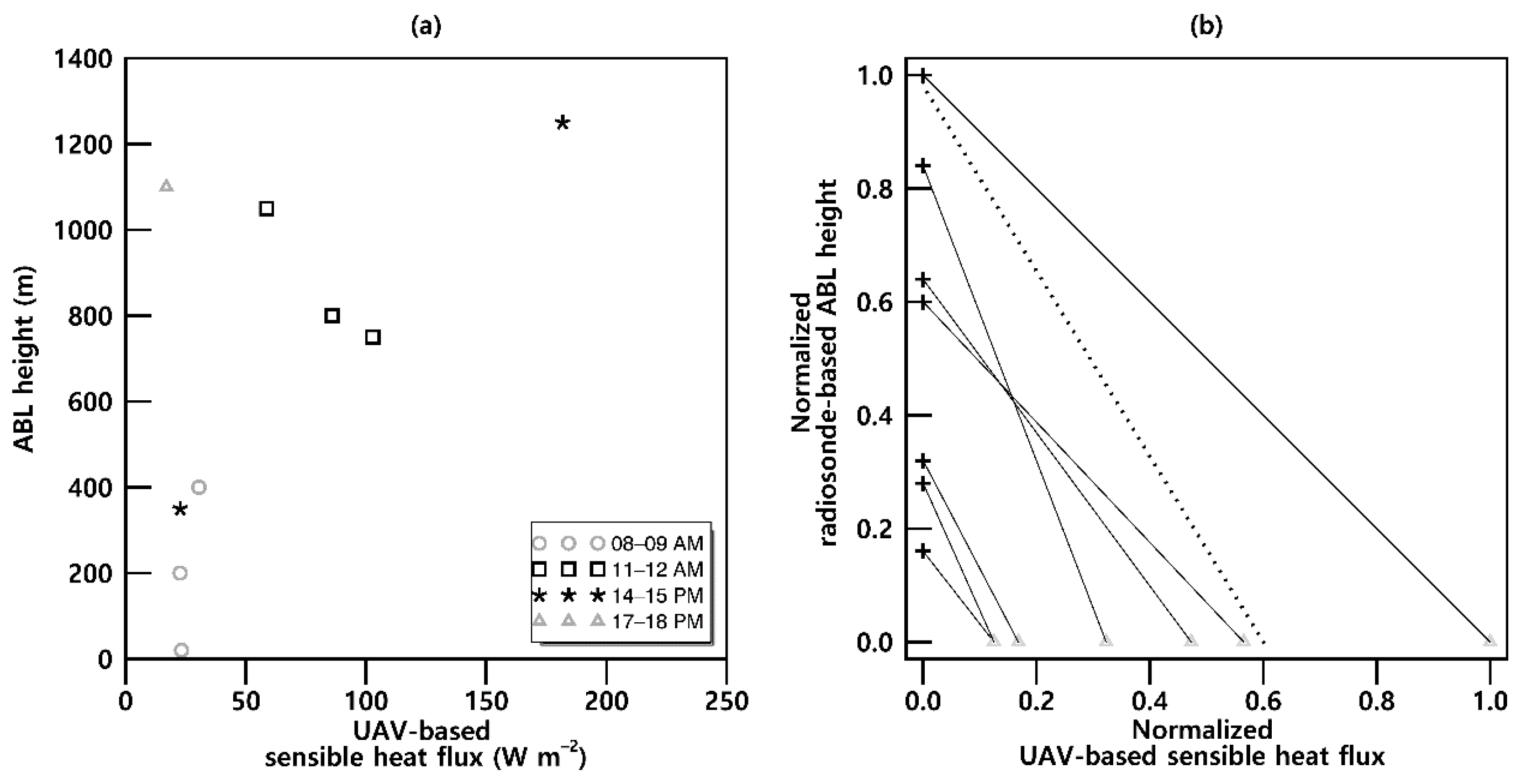
3.4. Atmospheric Boundary Layer Height Based on Rotary-Wing UAV Hovering
4. Conclusions
Author Contributions
Funding
Acknowledgments
Conflicts of Interest
References
- Arya, S.P. Introduction to Micrometeorology; Academic Press: San Diego, CA, USA, 1988; ISBN 9788578110796. [Google Scholar]
- Yi, C.; Davis, K.J.; Berger, B.W.; Bakwin, P.S.; Yi, C.; Davis, K.J.; Berger, B.W.; Bakwin, P.S. Long-term observations of the dynamics of the continental planetary boundary layer. J. Atmos. Sci. 2001, 58, 1288–1299. [Google Scholar] [CrossRef]
- Yi, C.; Davis, K.J.; Bakwin, P.S.; Denning, A.S.; Zhang, N.; Desai, A.; Lin, J.C.; Gerbig, C.; Yi, C. Observed covariance between ecosystem carbon exchange and atmospheric boundary layer dynamics at a site in northern Wisconsin. J. Geophys. Res. 2004, 109, D08302. [Google Scholar] [CrossRef]
- Kalverla, P.C.; Duine, G.J.; Steeneveld, G.J.; Hedde, T.; Kalverla, P.C.; Duine, G.J.; Steeneveld, G.J.; Hedde, T. Evaluation of the weather research and forecasting model in the Durance Valley complex terrain during the KASCADE field campaign. J. Appl. Meteorol. Climatol. 2016, 55, 861–882. [Google Scholar] [CrossRef]
- Lehner, M.; Whiteman, C.D.; Hoch, S.W.; Jensen, D.; Pardyjak, E.R.; Leo, L.S.; Di Sabatino, S.; Fernando, H.J.S.; Lehner, M.; Whiteman, C.D.; et al. A case study of the nocturnal boundary layer evolution on a slope at the foot of a desert mountain. J. Appl. Meteorol. Climatol. 2015, 54, 732–751. [Google Scholar] [CrossRef]
- Rennó, N.O.; Williams, E.R. Quasi-lagrangian measurements in convective boundary layer plumes and their implications for the calculation of CAPE. Mon. Weather Rev. 1995, 123, 2733–2742. [Google Scholar] [CrossRef]
- Spiess, T.; Bange, J.; Buschmann, M.; Vörsmann, P. First application of the meteorological Mini-UAV “M2AV”. Meteorol. Zeitschrift 2007, 16, 159–169. [Google Scholar] [CrossRef] [PubMed]
- Holland, G.J.; McGeer, T.; Youngren, H.; Holland, G.J.; McGeer, T.; Youngren, H. Autonomous aerosondes for economical atmospheric soundings anywhere on the globe. Bull. Am. Meteorol. Soc. 1992, 73, 1987–1998. [Google Scholar] [CrossRef]
- Valero, F.P.J.; Bucholtz, A.; Bush, B.C.; Pope, S.K.; Collins, W.D.; Flatau, P.; Strawa, A.; Gore, W.J.Y. Atmospheric radiation measurements enhanced shortwave experiment (ARESE): Experimental and data details. J. Geophys. Res. Atmos. 1997, 102, 29929–29937. [Google Scholar] [CrossRef]
- Lawrence, D.A.; Balsley, B.B.; Lawrence, D.A.; Balsley, B.B. High-resolution atmospheric sensing of multiple atmospheric variables using the DataHawk small airborne measurement system. J. Atmos. Ocean. Technol. 2013, 30, 2352–2366. [Google Scholar] [CrossRef]
- Martin, S.; Bange, J.; Beyrich, F. Meteorological profiling of the lower troposphere using the research UAV “M2AV Carolo”. Atmos. Meas. Tech. 2011, 4, 705–716. [Google Scholar] [CrossRef]
- Mayer, S.; Sandvik, A.; Jonassen, M.O.; Reuder, J. Atmospheric profiling with the UAS SUMO: A new perspective for the evaluation of fine-scale atmospheric models. Meteorol. Atmos. Phys. 2012, 116, 15–26. [Google Scholar] [CrossRef]
- van den Kroonenberg, A.; Martin, T.; Buschmann, M.; Bange, J.; Vörsmann, P. Measuring the wind vector using the autonomous mini aerial vehicle M2AV. J. Atmos. Ocean. Technol. 2008, 25, 1969–1982. [Google Scholar] [CrossRef]
- Shimura, T.; Inoue, M.; Tsujimoto, H.; Sasaki, K.; Iguchi, M.; Shimura, T.; Inoue, M.; Tsujimoto, H.; Sasaki, K.; Iguchi, M. Estimation of wind vector profile using a hexarotor unmanned aerial vehicle and its application to meteorological observation up to 1000 m above Surface. J. Atmos. Ocean. Technol. 2018, 35, 1621–1631. [Google Scholar] [CrossRef]
- Palomaki, R.T.; Rose, N.T.; van den Bossche, M.; Sherman, T.J.; De Wekker, S.F.J. Wind estimation in the lower atmosphere using multirotor aircraft. J. Atmos. Ocean. Technol. 2017, 34, 1183–1191. [Google Scholar] [CrossRef]
- Divitiis, N. Wind estimation on a lightweight vertical-takeoff-and-landing uninhabited vehicle. J. Aircr. 2003, 40, 759–767. [Google Scholar] [CrossRef]
- Molnar, A.; Stojcsics, D. New approach of the navigation control of small size UAVs. In Proceedings of the 19th International Workshop on Robotics in Alpe-Adria-Danube Region (RAAD 2010), Balatonfured, Hungary, 24–26 June 2010; IEEE: Budapest, Hungary, 2010; pp. 125–129. [Google Scholar]
- Pachter, M.; Ceccarelli, N.; Chandler, P. Estimating MAV’s heading and the wind speed and direction using GPS, inertial, and air speed measurements. In AIAA Guidance, Navigation and Control Conference and Exhibit; American Institute of Aeronautics and Astronautics: Hawaii, HI, USA, 2008. [Google Scholar]
- Rodriguez, A.; Andersen, E.; Bradley, J.; Taylor, C. Wind estimation using an optical flow sensor on a miniature air vehicle. In AIAA Guidance, Navigation and Control Conference and Exhibit; American Institute of Aeronautics and Astronautics: South Carolina, CA, USA, 2007. [Google Scholar]
- Brosy, C.; Krampf, K.; Zeeman, M.; Wolf, B.; Junkermann, W.; Schäfer, K.; Emeis, S.; Kunstmann, H. Simultaneous multicopter-based air sampling and sensing of meteorological variables. Atmos. Meas. Tech. 2017, 10, 2773–2784. [Google Scholar] [CrossRef]
- Neumann, P.P.; Bartholmai, M. Real-time wind estimation on a micro unmanned aerial vehicle using its inertial measurement unit. Sensors Actuators A Phys. 2015, 235, 300–310. [Google Scholar] [CrossRef]
- Bonin, T.; Chilson, P.; Zielke, B.; Fedorovich, E. Observations of the Early Evening Boundary-Layer Transition Using a Small Unmanned Aerial System. Bound-Lay Meteorol. 2013, 146, 119–132. [Google Scholar] [CrossRef]
- Reineman, B.D.; Lenain, L.; Statom, N.M.; Melville, W.K.; Reineman, B.D.; Lenain, L.; Statom, N.M.; Melville, W.K. Development and testing of instrumentation for UAV-based flux measurements within terrestrial and marine atmospheric boundary layers. J. Atmos. Ocean. Technol. 2013, 30, 1295–1319. [Google Scholar] [CrossRef]
- Knuth, S.L.; Cassano, J.J. Estimating sensible and latent heat fluxes using the integral method from in situ aircraft measurements. J. Atmos. Ocean. Technol. 2014, 31, 1964–1981. [Google Scholar] [CrossRef]
- Båserud, L.; Reuder, J.; Jonassen, M.O.; Kral, S.T.; Paskyabi, M.B.; Lothon, M. Proof of concept for turbulence measurements with the RPAS SUMO during the BLLAST campaign. Atmos. Meas. Tech. 2016, 9, 4901–4913. [Google Scholar] [CrossRef]
- Garratt, J.R. Review: The atmospheric boundary layer. Earth-Science Rev. 1994, 37, 89–134. [Google Scholar] [CrossRef]
- Deardorff, J.W. Parameterization of the planetary boundary layer for use in general circulation models 1. Mon. Weather Rev. 1972, 100, 93–106. [Google Scholar] [CrossRef]
- Katz, J.; Zhu, P. Evaluation of surface layer flux parameterizations using in-situ observations. Atmos. Res. 2017, 194, 150–163. [Google Scholar] [CrossRef]
- Monin, A.S.; Obukhov, A.M. Basic laws of turbulent mixing in the surface layer of the atmosphere. Tr. Akad. Nauk SSSR Geophiz. Inst. 1954, 24, 163–187. [Google Scholar]
- Stanhill, G. A simple instrument for the field measurement of turbulent diffusion flux. J. Appl. Meteorol. 1969, 8, 509–513. [Google Scholar] [CrossRef]
- Brümmer, B.; Schröder, D.; Launiainen, J.; Vihma, T.; Smedman, A.S.; Magnusson, M. Temporal and spatial variability of surface fluxes over the ice edge zone in the northern Baltic Sea. J. Geophys. Res. 2002, 107, 3096. [Google Scholar] [CrossRef]
- Verkaik, J.W.; Holtslag, A.A.M. Wind profiles, momentum fluxes and roughness lengths at Cabauw revisited. Bound-Lay Meteorol. 2007, 122, 701–719. [Google Scholar] [CrossRef]
- Businger, J.A.; Wyngaard, J.C.; Izumi, Y.; Bradley, E.F.; Businger, J.A.; Wyngaard, J.C.; Izumi, Y.; Bradley, E.F. Flux-profile relationships in the atmospheric surface layer. J. Atmos. Sci. 1971, 28, 181–189. [Google Scholar] [CrossRef]
- Launiainen, J.; Vihma, T. Derivation of turbulent surface fluxes—An iterative flux-profile method allowing arbitrary observing heights. Environ. Softw. 1990, 5, 113–124. [Google Scholar] [CrossRef]
- De Bruin, H.A.R.; Van Den Hurk, B.J.J.M.; Kohsiek, W. The scintillation method tested over a dry vineyard area. Bound-Lay Meteorol. 1995, 76, 25–40. [Google Scholar] [CrossRef]
- Kanda, M.; Moriwaki, R.; Roth, M.; Oke, T. Area-averaged sensible heat flux and a new method to determine Zero-Plane displacement length over an urban surface using scintillometry. Bound-Laye Meteorol. 2002, 105, 177–193. [Google Scholar] [CrossRef]
- Nieveen, J.P.; Green, A.E. Measuring sensible heat flux density over pasture using the ct2-Profile method. Bound-Lay Meteorol. 1999, 91, 23–35. [Google Scholar] [CrossRef]
- Weiss, A.I.; Hennes, M.; Rotach, M.W. Derivation of refractive index and temperature gradients from optical scintillometry to correct atmospherically induced errors for highly precise geodetic measurements. Surv. Geophys. 2001, 22, 589–596. [Google Scholar] [CrossRef]
- Arain, B.; Kendoul, F. Real-time wind speed estimation and compensation for improved flight. IEEE Trans. Aerosp. Electron. Syst. 2014, 50, 1599–1606. [Google Scholar] [CrossRef]
- Stull, R.B. An Introduction to Boundary Layer Meteorology; Kluwer Academic Publishers: Dordrecht, The Netherlands, 1988; ISBN 978-94-009-3027-8. [Google Scholar]
- Alvarado, M.; Gonzalez, F.; Fletcher, A.; Doshi, A. Towards the development of a low cost airborne sensing system to monitor dust particles after blasting at open-pit mine sites. Sensors 2015, 15, 19667–19687. [Google Scholar] [CrossRef] [PubMed]
- Vickers, D.; Mahrt, L.; Vickers, D.; Mahrt, L. Quality control and flux sampling problems for tower and aircraft data. J. Atmos. Ocean. Technol. 1997, 14, 512–526. [Google Scholar] [CrossRef]
- Lee, T.R.; Buban, M.; Dumas, E.; Baker, C.B.; Lee, T.R.; Buban, M.; Dumas, E.; Baker, C.B. A new technique to estimate sensible heat fluxes around micrometeorological towers using small unmanned aircraft systems. J. Atmos. Ocean. Technol. 2017, 34, 2103–2112. [Google Scholar] [CrossRef]
- Zhang, W.; Guo, J.; Miao, Y.; Liu, H.; Song, Y.; Fang, Z.; He, J.; Lou, M.; Yan, Y.; Li, Y.; et al. On the summertime planetary boundary layer with different thermodynamic stability in China: A radiosonde perspective. J. Clim. 2018, 31, 1451–1465. [Google Scholar] [CrossRef]
- Wang, X.Y.; Wang, K.C. Estimation of atmospheric mixing layer height from radiosonde data. Atmos. Meas. Tech. 2014, 7, 1701–1709. [Google Scholar] [CrossRef]
- Seidel, D.J.; Ao, C.O.; Li, K. Estimating climatological planetary boundary layer heights from radiosonde observations: Comparison of methods and uncertainty analysis. J. Geophys. Res. 2010, 115, D16113. [Google Scholar] [CrossRef]
- Zhang, Y.; Seidel, D.J.; Zhang, S.; Zhang, Y.; Seidel, D.J.; Zhang, S. Trends in planetary boundary layer height over Europe. J. Clim. 2013, 26, 10071–10076. [Google Scholar] [CrossRef]
- Lenschow, D.H.; Li, X.S.; Zhu, C.J.; Stankov, B.B. The Stably Stratified Boundary Layer over the Great Plains. In Topics in Micrometeorology. A Festschrift for Arch Dyer; Springer: Dordrecht, The Netherlands, 1988; pp. 95–121. [Google Scholar]
- Mahrt, L. Vertical structure and turbulence in the very stable boundary layer. J. Atmos. Sci. 1985, 42, 2333–2349. [Google Scholar] [CrossRef]
- Tjernström, M. Turbulence length scales in stably stratified free shear flow analyzed from slant aircraft profiles. J. Appl. Meteorol. 1993, 32, 948–963. [Google Scholar] [CrossRef]
- Nieuwstadt, F. The computation of the friction velocity u * and the temperature scale T * from temperature and wind velocity profiles by least-square methods. Bound-Lay Meteorol. 1978, 14, 235–246. [Google Scholar] [CrossRef]


| Site | Period | Surface | d0 (m) | z0m (m) | Synoptic Condition | Main Instruments |
|---|---|---|---|---|---|---|
| GH1 | 2006.08.08–2006.08.11 | Reed | 2.1 | 2.8 × 10⁻¹ | North pacific anticyclone | USA |
| GH2 | 2005.02.23–2005.02.25 | Reed | 1.7 | 1.0 × 10⁻¹ | Siberian anticyclone | USA |
| GR1 | 2012.10.08–2012.10.11 | Rice | 0.6 | 8.5 × 10⁻² | Migratory anticyclone | USA |
| GR2 | 2012.10.14–2012.10.16 | Cut paddy | 0.01 | 5.6 × 10⁻² | Migratory anticyclone | USA |
| KHR | 2012.10.01–2012.10.03 | Water | 0 | 1.0 × 10⁻³ | Migratory anticyclone | USA, SLS20 |
| SYR | 2013.03.14–2013.03.16 | Water | 0 | 1.0 × 10⁻³ | Migratory anticyclone | USA, SLS20 |
| CHR | 2016.07.09–2016.07.10 | Asphalt | 0 | 3.0 × 10⁻² | North pacific anticyclone | RS, USA, UAV |
| WON | 2016.07.11–2016.07.14 | Stone | 0 | 0.2 × 10⁻² | North pacific anticyclone | RS, USA, UAV |
| SOK | 2017.02.09–2017.03.15 | Stone | 0 | 2.0 × 10⁻² | Migratory anticyclone | RS, USA, UAV |
| BOS | 2018.09.10–2018.09.12 | Grass | 0.3 | 1.2 × 10⁻² | Migratory anticyclone | RS, USA, UAV |
| YHI | 2018.11.27–2018.12.05 | Trees | 2.0 | 1.7 × 10⁻¹ | Siberian anticyclone | RS, USA, UAV |
© 2019 by the authors. Licensee MDPI, Basel, Switzerland. This article is an open access article distributed under the terms and conditions of the Creative Commons Attribution (CC BY) license (http://creativecommons.org/licenses/by/4.0/).
Share and Cite
Kim, M.-S.; Kwon, B.H. Estimation of Sensible Heat Flux and Atmospheric Boundary Layer Height Using an Unmanned Aerial Vehicle. Atmosphere 2019, 10, 363. https://doi.org/10.3390/atmos10070363
Kim M-S, Kwon BH. Estimation of Sensible Heat Flux and Atmospheric Boundary Layer Height Using an Unmanned Aerial Vehicle. Atmosphere. 2019; 10(7):363. https://doi.org/10.3390/atmos10070363
Chicago/Turabian StyleKim, Min-Seong, and Byung Hyuk Kwon. 2019. "Estimation of Sensible Heat Flux and Atmospheric Boundary Layer Height Using an Unmanned Aerial Vehicle" Atmosphere 10, no. 7: 363. https://doi.org/10.3390/atmos10070363
APA StyleKim, M.-S., & Kwon, B. H. (2019). Estimation of Sensible Heat Flux and Atmospheric Boundary Layer Height Using an Unmanned Aerial Vehicle. Atmosphere, 10(7), 363. https://doi.org/10.3390/atmos10070363