Spatio-Temporal Consistency Evaluation of XCO2 Retrievals from GOSAT and OCO-2 Based on TCCON and Model Data for Joint Utilization in Carbon Cycle Research


Abstract
1. Introduction
2. Materials and Methods
2.1. GOSAT
2.2. OCO-2
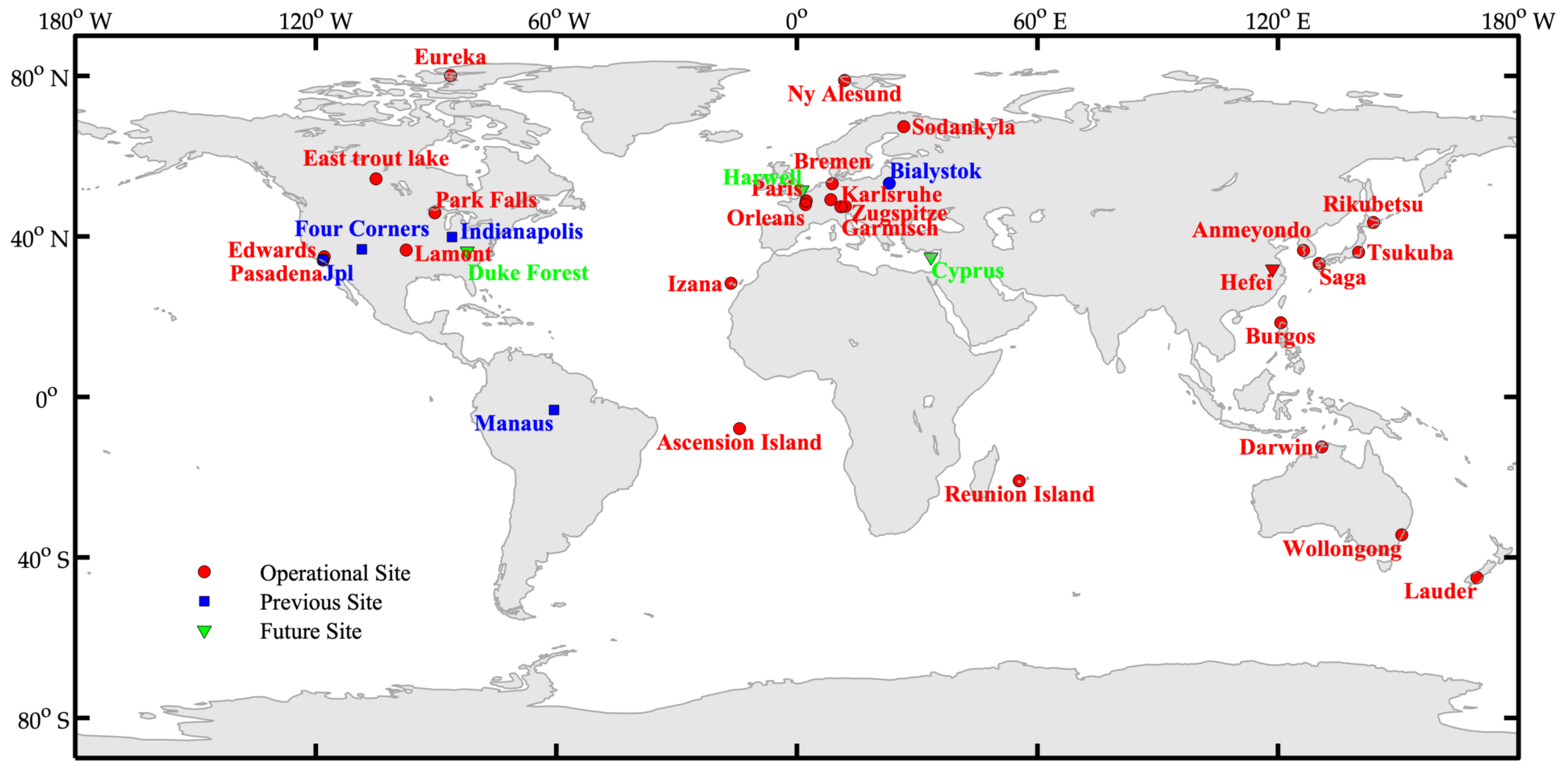
2.3. TCCON
2.4. CarbonTracker
2.5. Spatiotemporal Collocation Criterion
3. Results
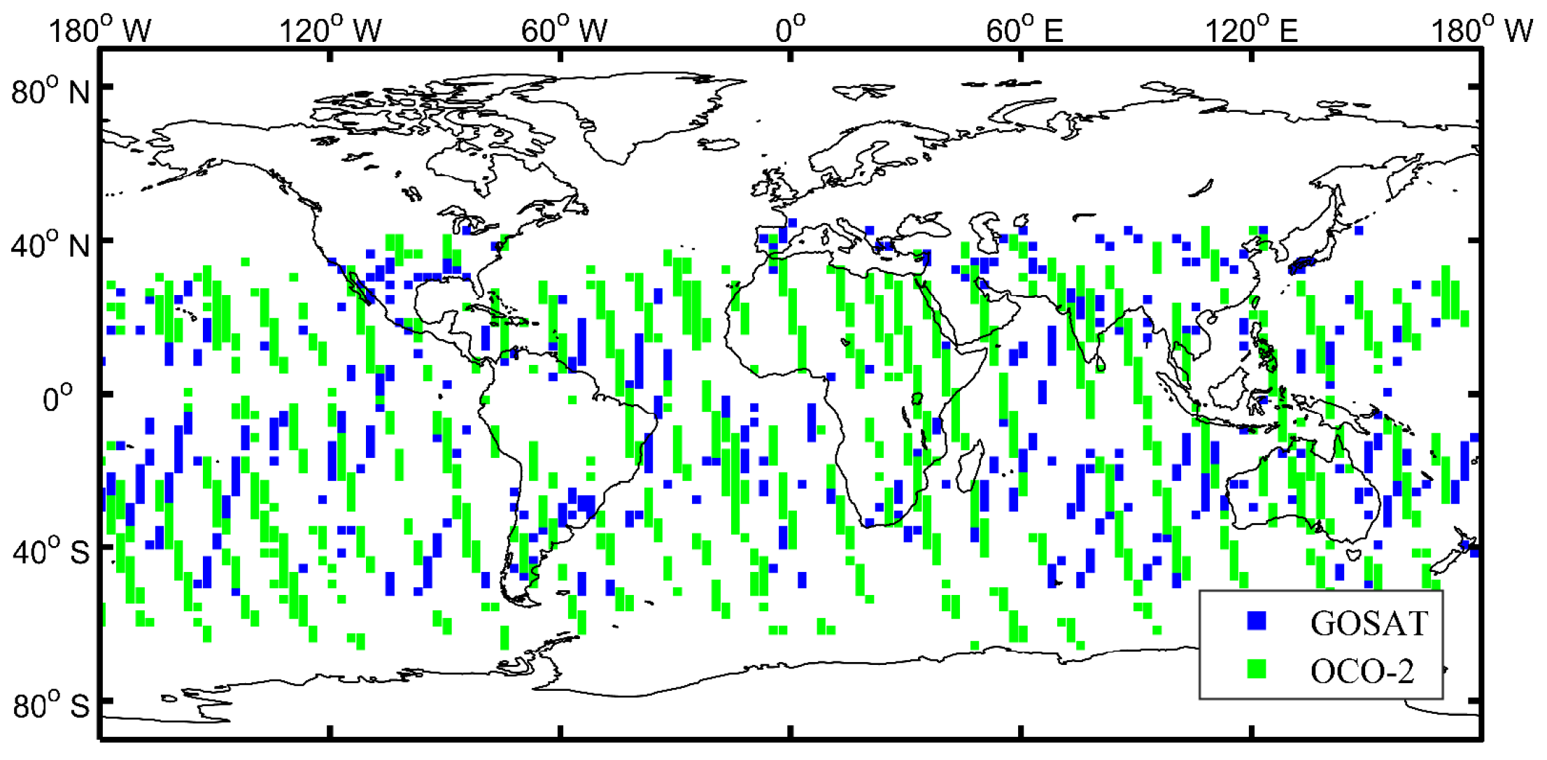
3.1. Spatial Coverage of GOSAT and OCO-2 Observations
3.2. The Inter-Comparison of GOSAT, OCO-2 and TCCON
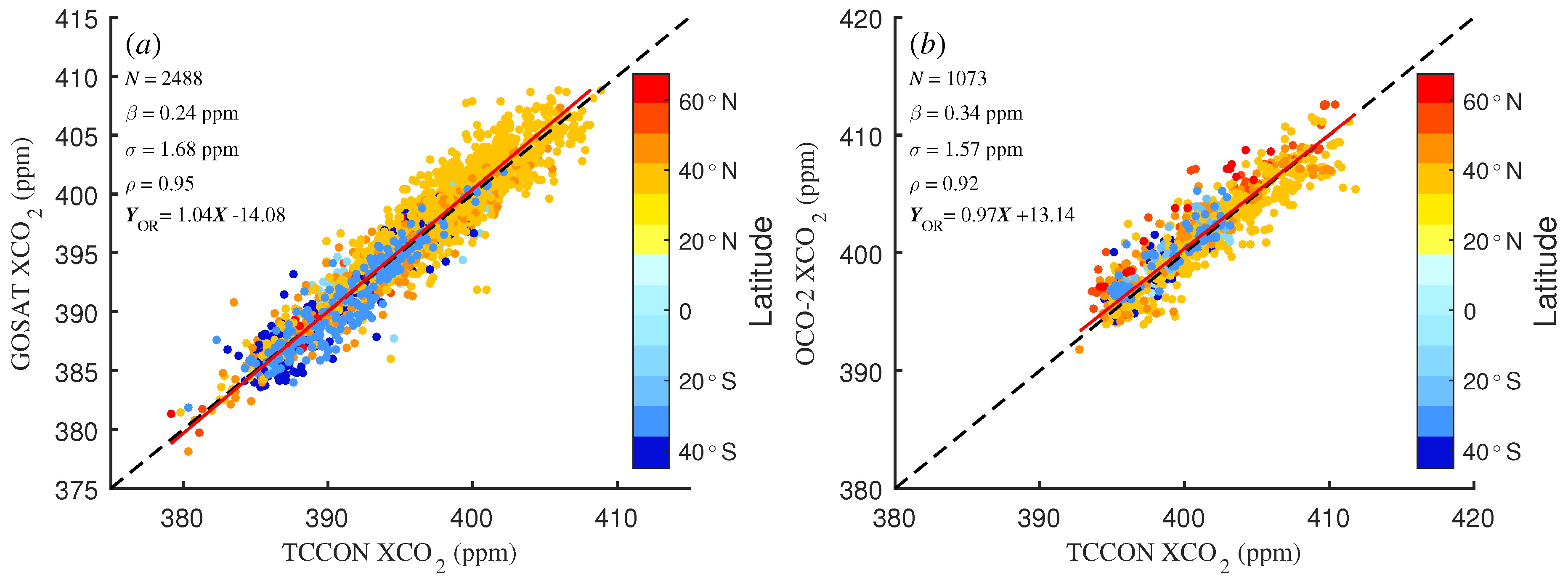
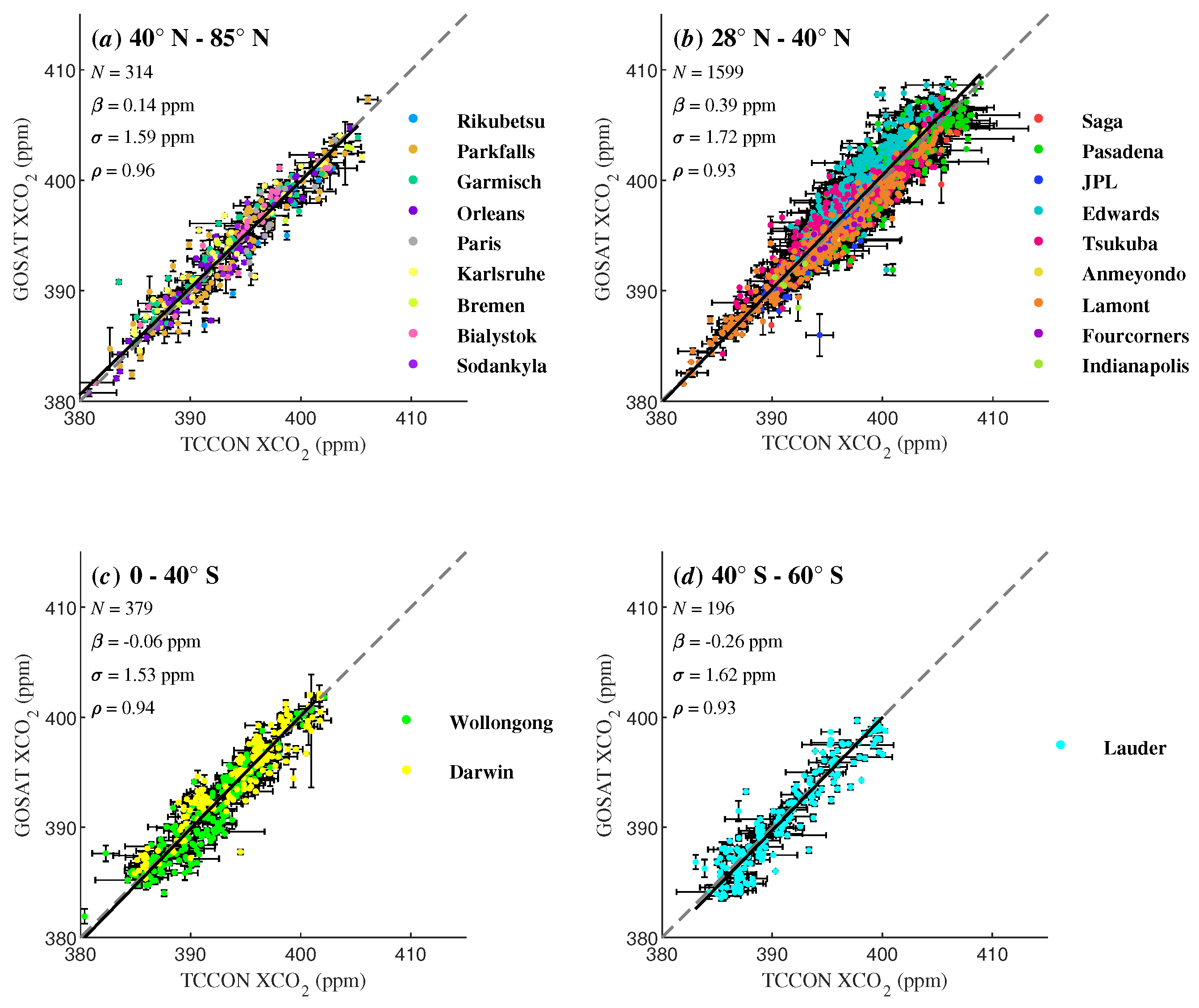
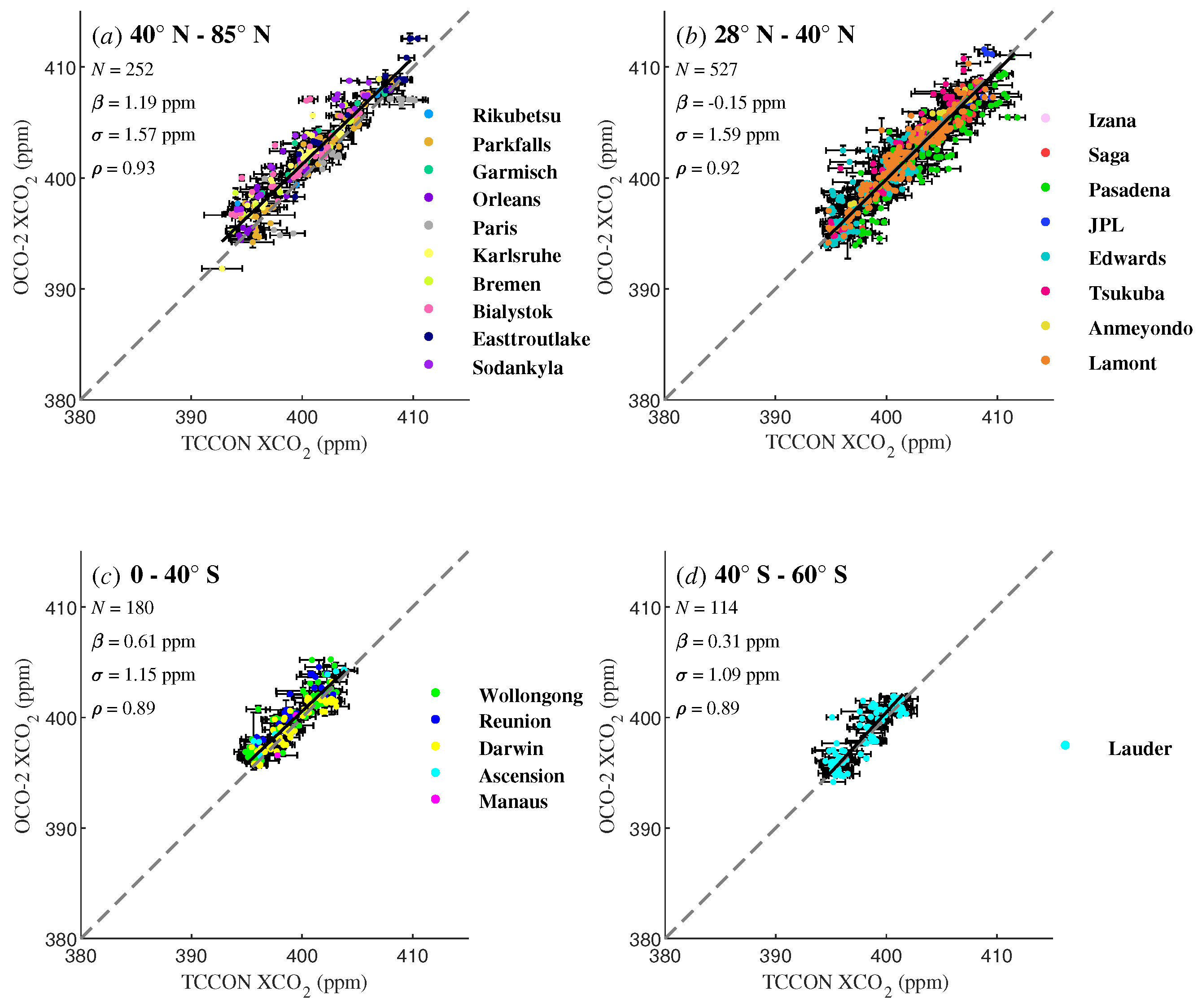
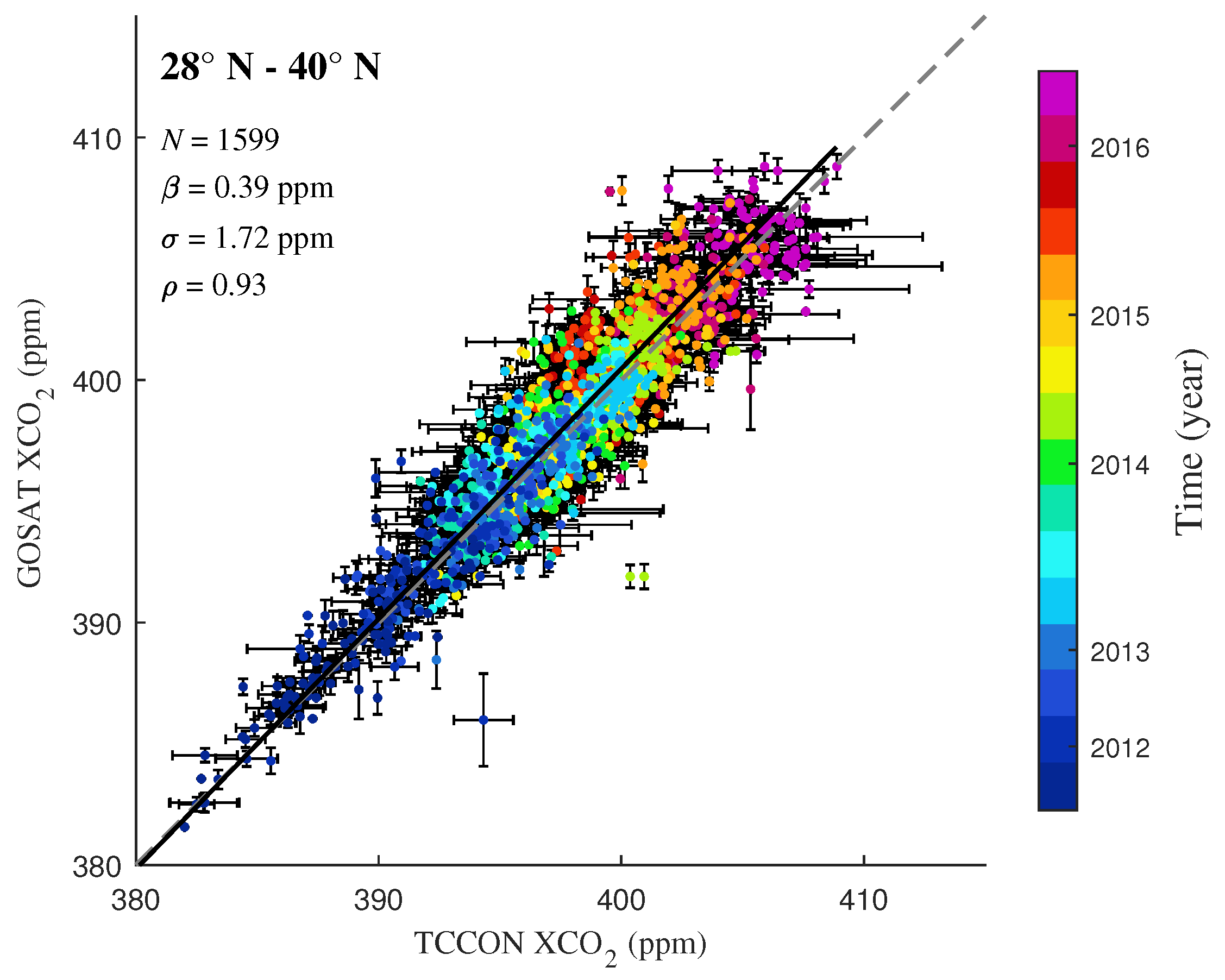
3.2.1. Validation of the OCO-2 and GOSAT XCO Products Using TCCON Data
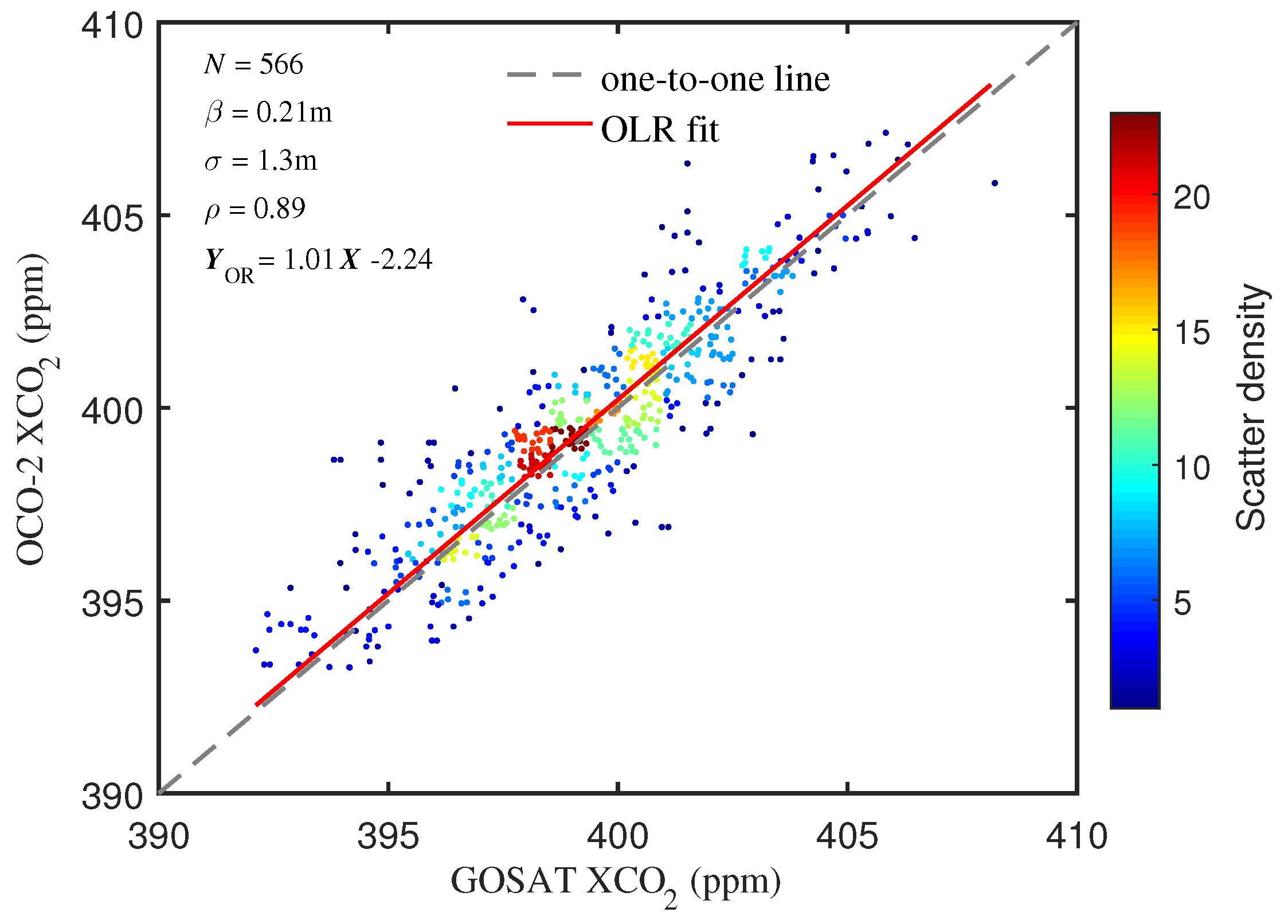
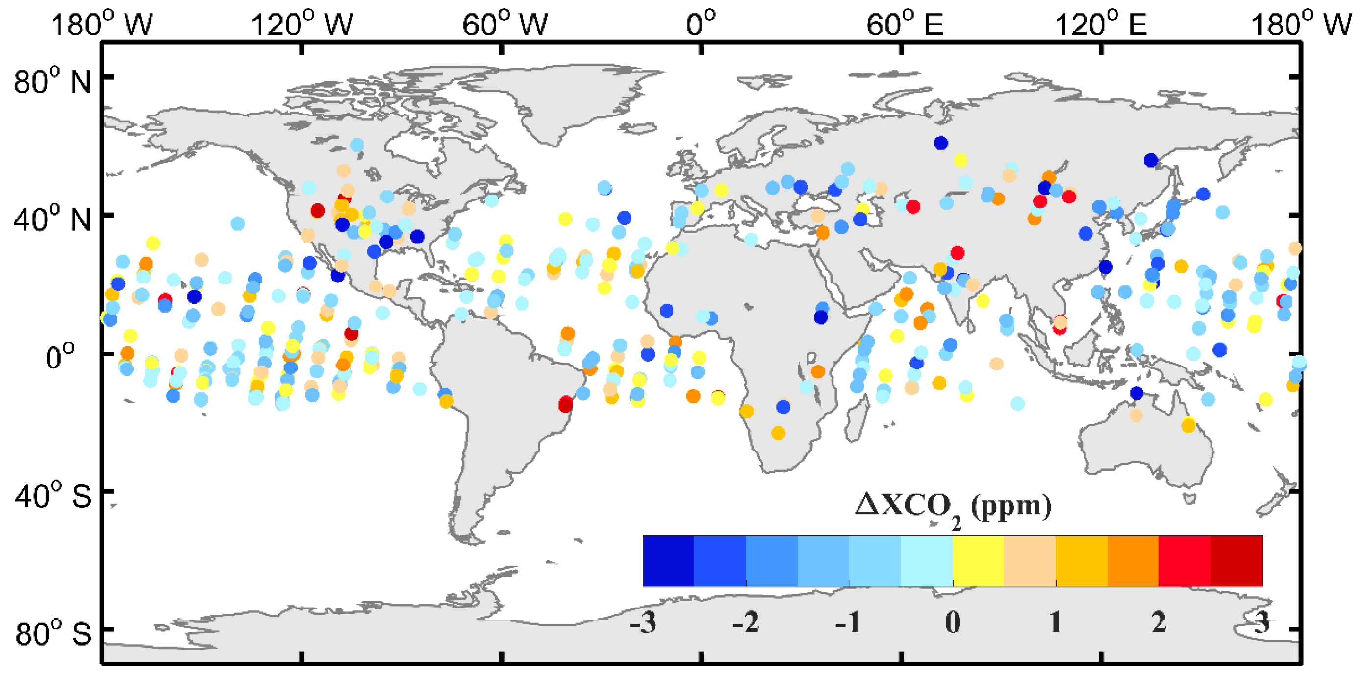
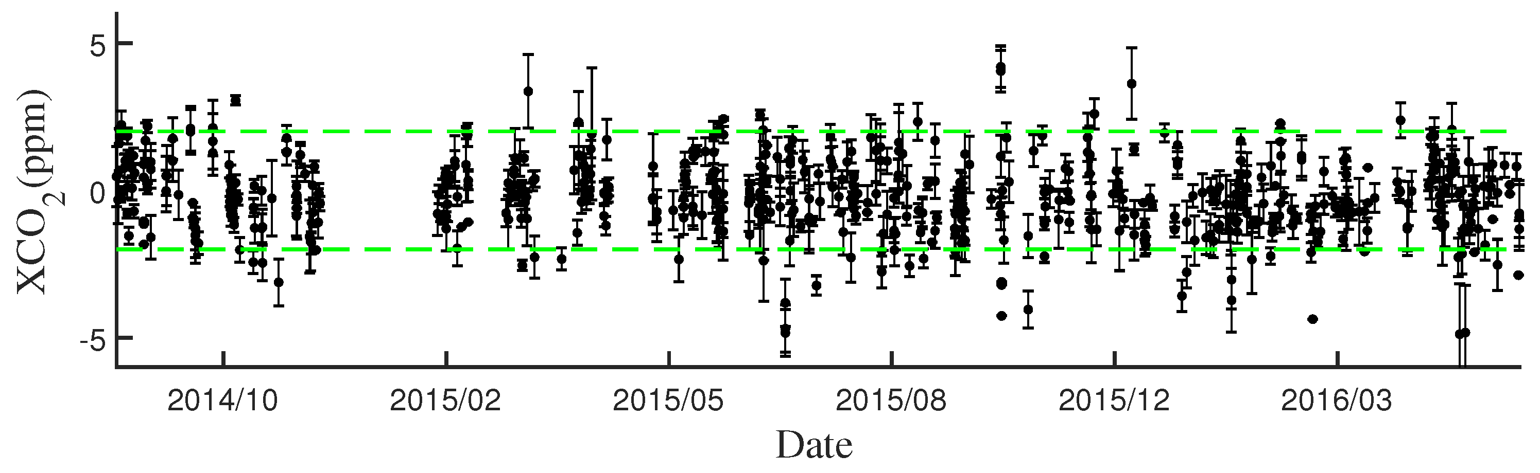
3.2.2. The Cross Comparison between the GOSAT and OCO-2 XCO
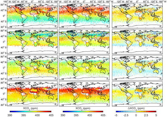
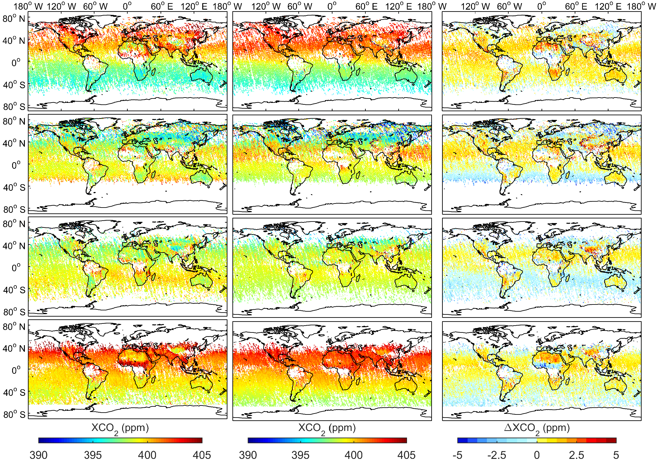
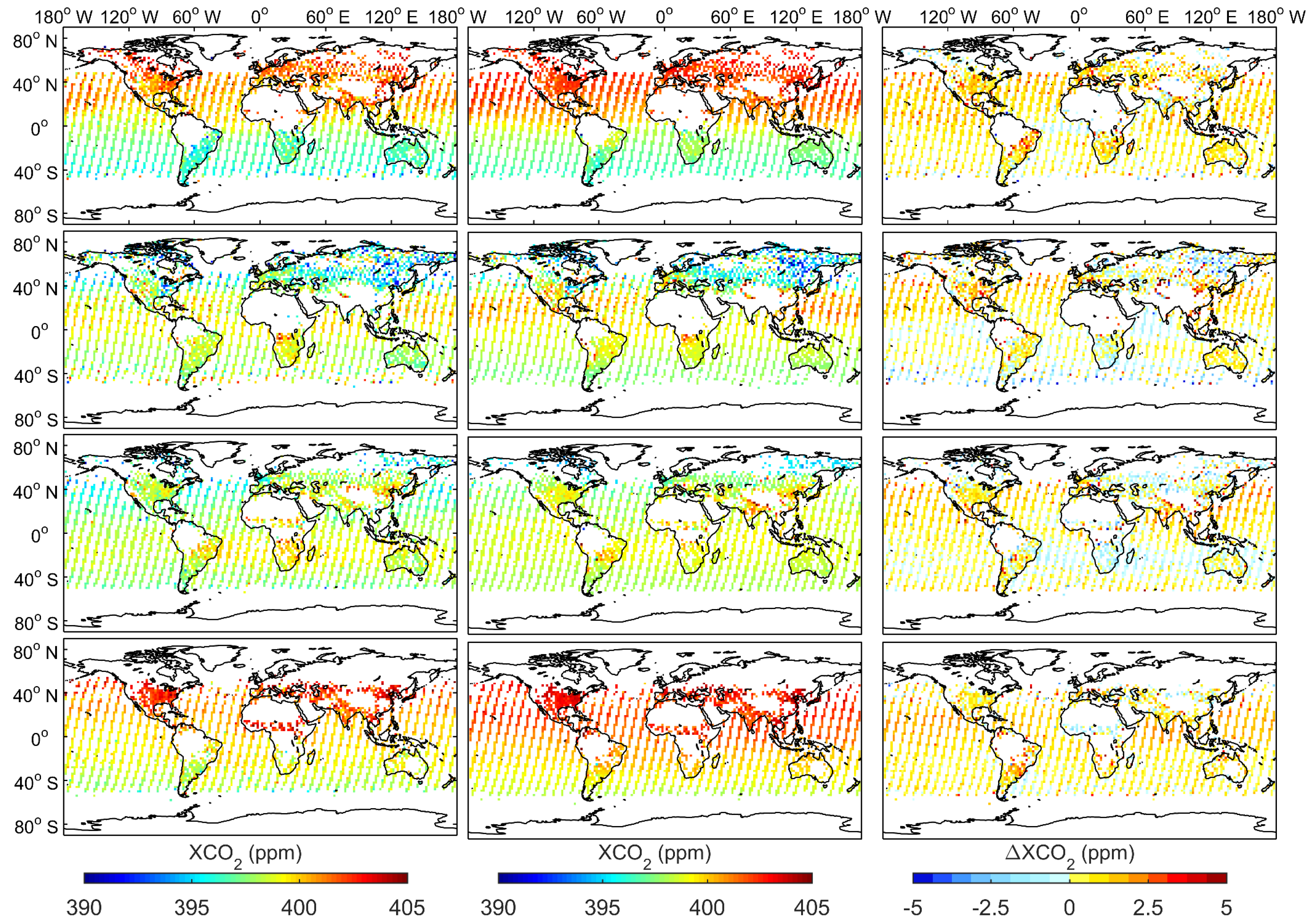
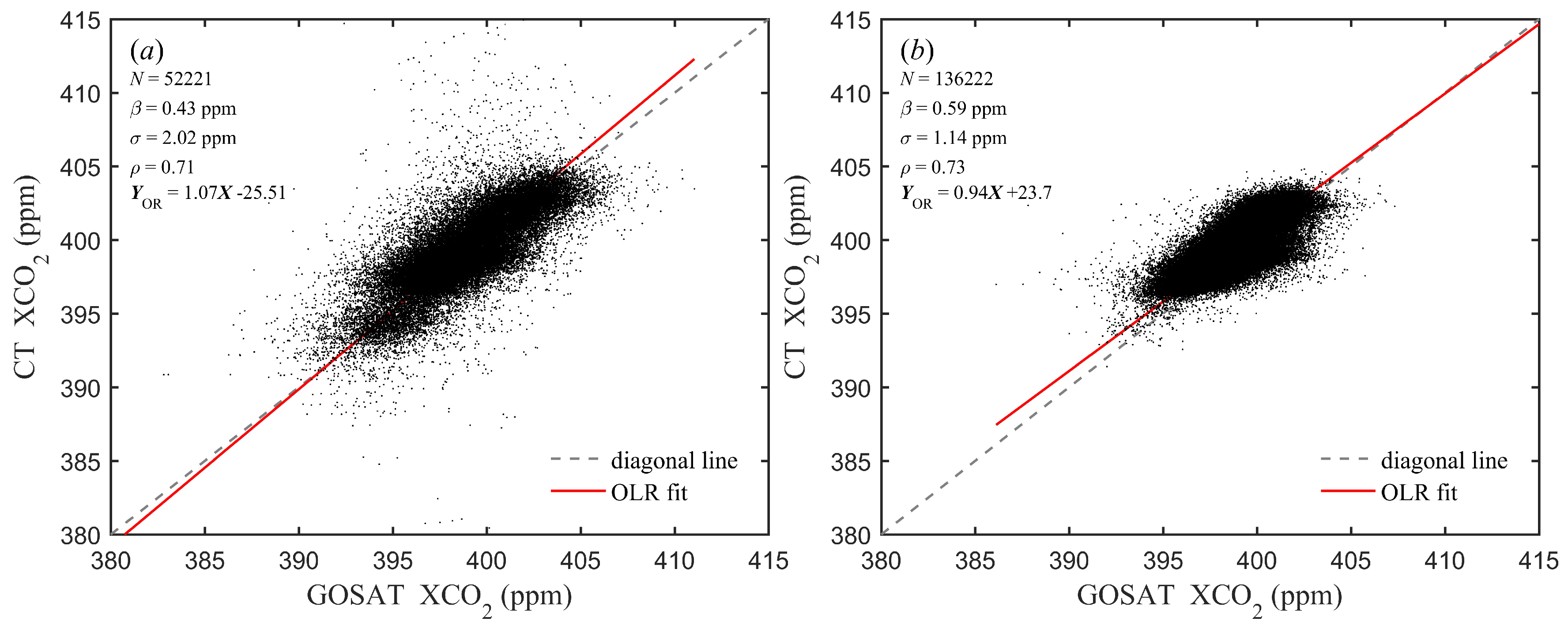
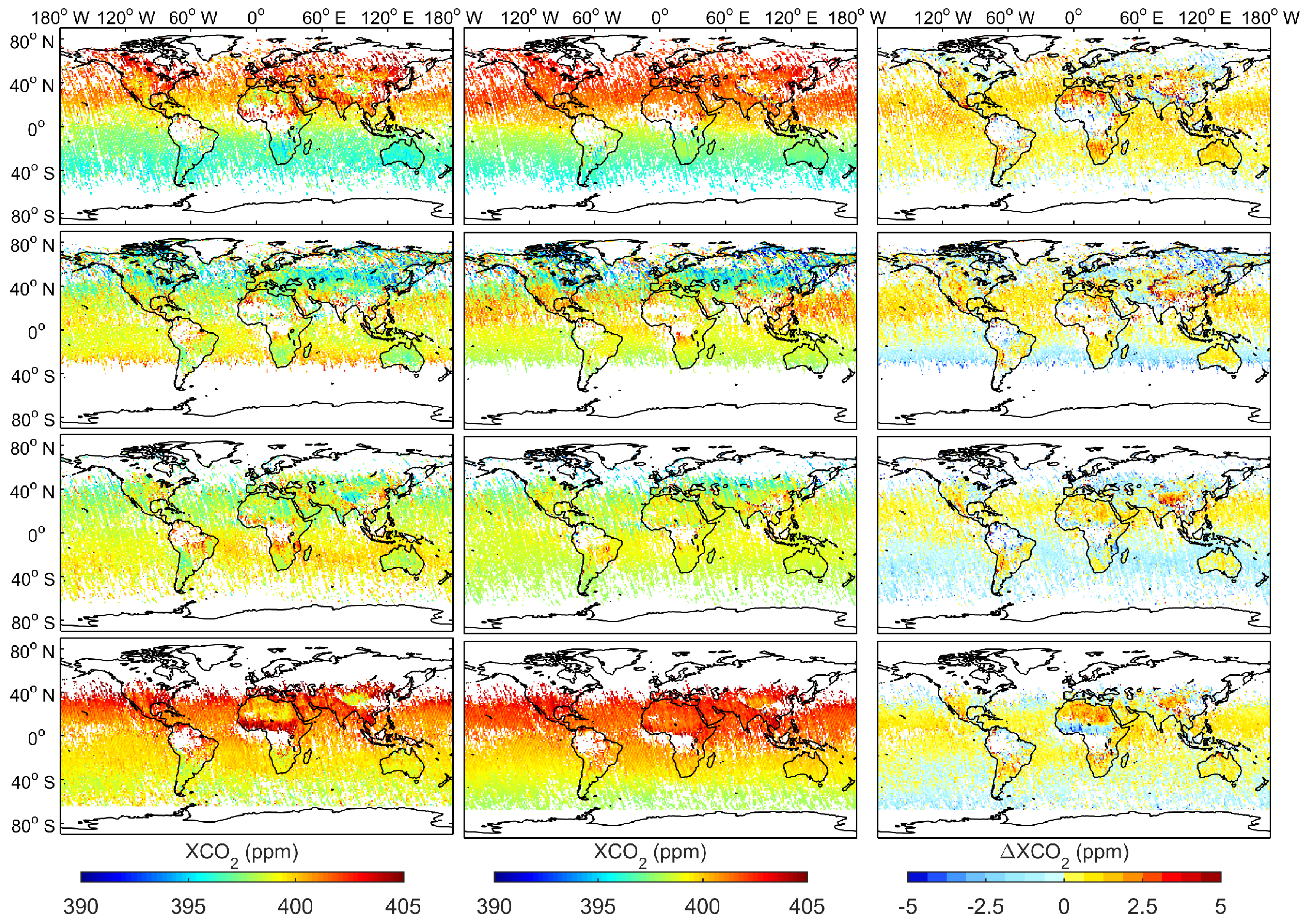
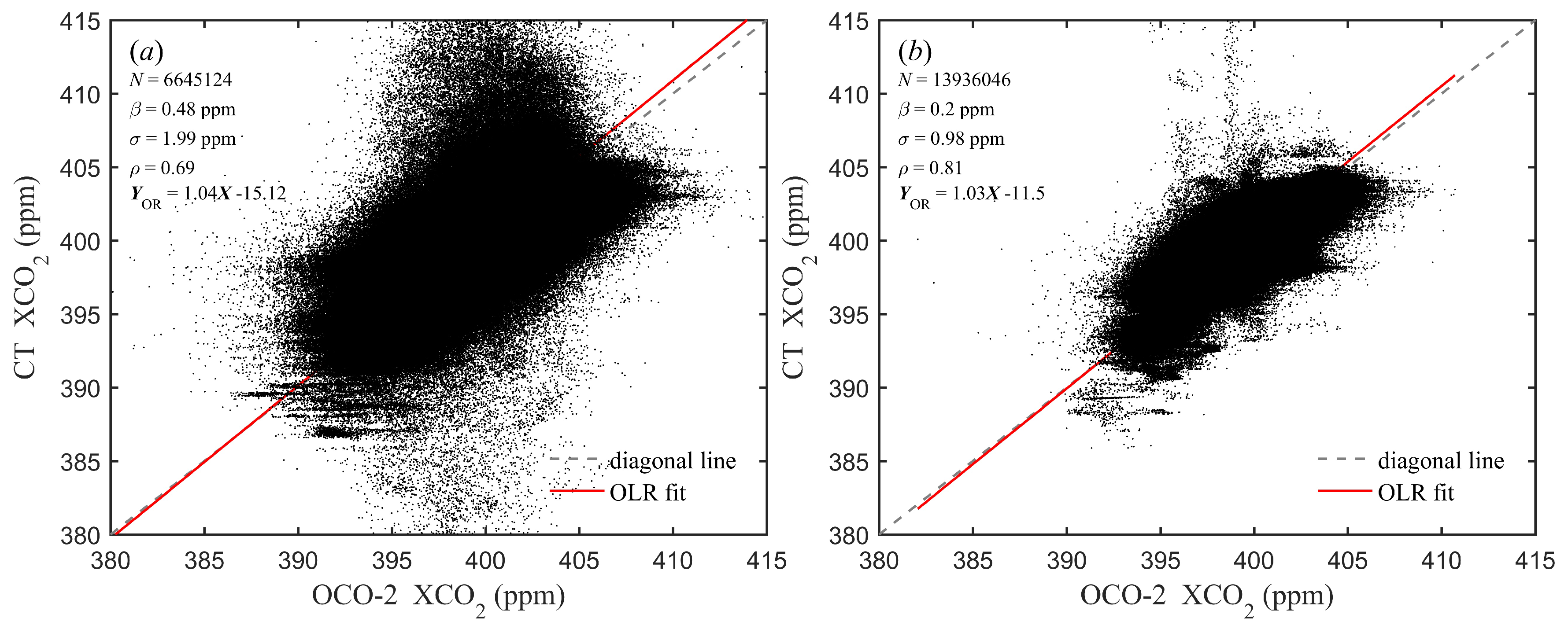
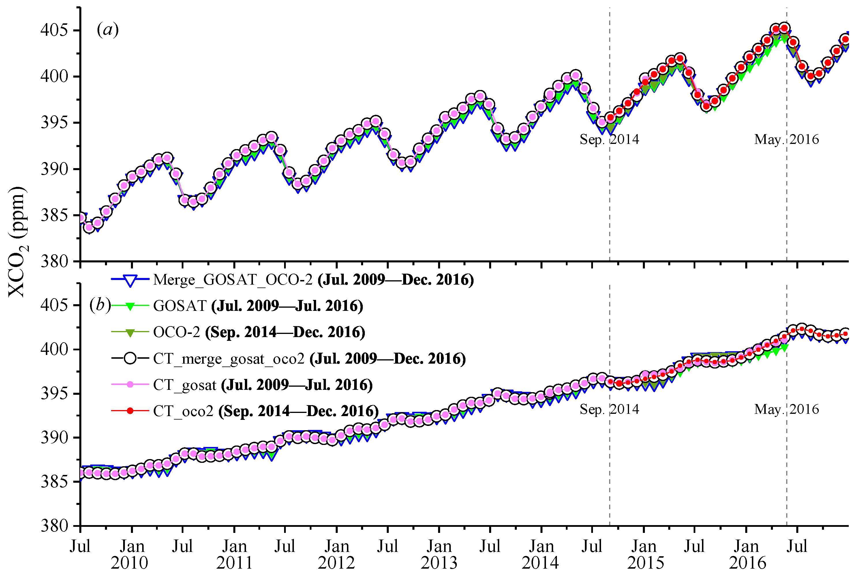
3.3. Comparison of XCO Satellite Retrievals with XCO Computed from a Model
4. Conclusions and Discussion
Author Contributions
Funding
Acknowledgments
Conflicts of Interest
References
- IPCC. Climate Change 2013: The Physical Science Basis. Contribution of Working Group I to the Fifth Assessment Report of the Intergovernmental Panel on Climate Change; Cambridge University Press: Cambridge, UK; New York, NY, USA, 2013; p. 1535. [Google Scholar] [CrossRef]
- Deng, F.; Jones, D.B.A.; Henze, D.K.; Bousserez, N.; Bowman, K.W.; Fisher, J.B.; Nassar, R.; O’Dell, C.; Wunch, D.; Wennberg, P.O.; et al. Inferring regional sources and sinks of atmospheric CO2 from GOSAT XCO2 data. Atmos. Chem. Phys. 2014, 14, 3703–3727. [Google Scholar] [CrossRef]
- Solomon, S.; Qin, D.; Manning, M.; Chen, Z.; Marquis, M.; Averyt, K.B.; Tignor, M.; Miller, H.E. Contribution of Working Group I to the Fourth Assessment Report of the Intergovernmental Panel on Climate Change; Cambridge University Press: Cambridge, UK; New York, NY, USA, 2007. [Google Scholar]
- Bousquet, P.; Ciais, P.; Miller, J.B.; Dlugokencky, E.J.; Hauglustaine, D.A.; Prigent, C.; Van der Werf, G.R.; Peylin, P.; Brunke, E.G.; Carouge, C.; et al. Contribution of anthropogenic and natural sources to atmospheric methane variability. Nature 2006, 443, 439–443. [Google Scholar] [CrossRef] [PubMed]
- Marquis, M.; Tans, P. Climate change—Carbon crucible. Science 2008, 320, 460–461. [Google Scholar] [CrossRef] [PubMed]
- Baker, D.F.; Bosch, H.; Doney, S.C.; O’Brien, D.; Schimel, D.S. Carbon source/sink information provided by column CO2 measurements from the Orbiting Carbon Observatory. Atmos. Chem. Phys. 2010, 10, 4145–4165. [Google Scholar] [CrossRef]
- Alexe, M.; Bergamaschi, P.; Segers, A.; Detmers, R.; Butz, A.; Hasekamp, O.; Guerlet, S.; Parker, R.; Boesch, H.; Frankenberg, C.; et al. Inverse modelling of CH4 emissions for 2010-2011 using different satellite retrieval products from GOSAT and SCIAMACHY. Atmos. Chem. Phys. 2015, 15, 113–133. [Google Scholar] [CrossRef]
- Yang, Z.; Washenfelder, R.A.; Keppel-Aleks, G.; Krakauer, N.Y.; Randerson, J.T.; Tans, P.P.; Sweeney, C.; Wennberg, P.O. New constraints on Northern Hemisphere growing season net flux. Geophys. Res. Lett. 2007, 34. [Google Scholar] [CrossRef]
- Keppel-Aleks, G.; Wennberg, P.O.; Schneider, T. Sources of variations in total column carbon dioxide. Atmos. Chem. Phys. 2011, 11, 3581–3593. [Google Scholar] [CrossRef]
- Kuze, A.; Suto, H.; Nakajima, M.; Hamazaki, T. Thermal and near infrared sensor for carbon observation Fourier-transform spectrometer on the Greenhouse Gases Observing Satellite for greenhouse gases monitoring. Appl. Opt. 2009, 48, 6716–6733. [Google Scholar] [CrossRef]
- Crisp, D.; Atlas, R.M.; Breon, F.M.; Brown, L.R.; Burrows, J.P.; Ciais, P.; Connor, B.J.; Doney, S.C.; Fung, I.Y.; Jacob, D.J.; et al. The orbiting carbon observatory (OCO) mission. Adv. Space Res. 2004, 34, 700–709. [Google Scholar] [CrossRef]
- Crisp, D. Measuring Atmospheric Carbon Dioxide from Space with the Orbiting Carbon Observatory-2 (OCO-2). In Earth Observing Systems XX, Proceedings of the SPIE Optical Engineering + Applications, San Diego, CA, USA, 9–13 August 2015; Butler, J.J., Xiong, X., Gu, X., Eds.; International Society for Optical Engineering: San Diego, CA, USA, 2015; Volume 9607. [Google Scholar] [CrossRef]
- Liang, A.; Gong, W.; Han, G.; Xiang, C. Comparison of Satellite-Observed XCO2 from GOSAT, OCO-2, and Ground-Based TCCON. Remote Sens. 2017, 9, 1033. [Google Scholar] [CrossRef]
- Chevallier, F.; Engelen, R.J.; Peylin, P. The contribution of AIRS data to the estimation of CO2 sources and sinks. Geophys. Res. Lett. 2005, 32. [Google Scholar] [CrossRef]
- Bergamaschi, P.; Frankenberg, C.; Meirink, J.F.; Krol, M.; Villani, M.G.; Houweling, S.; Dentener, F.; Dlugokencky, E.J.; Miller, J.B.; Gatti, L.V.; et al. Inverse modeling of global and regional CH4 emissions using SCIAMACHY satellite retrievals. J. Geophys. Res.-Atmos. 2009, 114. [Google Scholar] [CrossRef]
- Takagi, H.; Saeki, T.; Oda, T.; Saito, M.; Valsala, V.; Belikov, D.; Saito, R.; Yoshida, Y.; Morino, I.; Uchino, O.; et al. On the Benefit of GOSAT Observations to the Estimation of Regional CO2 Fluxes. Sci. Online Lett. Atmos. 2011, 7, 161–164. [Google Scholar]
- Saeki, T.; Maksyutov, S.; Saito, M.; Valsala, V.; Oda, T.; Andres, R.J.; Belikov, D.; Tans, P.; Dlugokencky, E.; Yoshida, Y.; et al. Inverse Modeling of CO2 Fluxes Using GOSAT Data and Multi-Year Ground-Based Observations. Sci. Online Lett. Atmos. 2013, 9, 45–50. [Google Scholar] [CrossRef]
- Basu, S.; Guerlet, S.; Butz, A.; Houweling, S. Global CO2 fluxes estimated from GOSAT retrievals of total column CO2. Atmos. Chem. Phys. 2013, 13, 8695–8717. [Google Scholar] [CrossRef]
- Chen, J.M.; Mo, G.; Deng, F. A joint global carbon inversion system using both CO2 and 13CO2 atmospheric concentration data. Geosci. Model Dev. 2017, 10, 1131–1156. [Google Scholar] [CrossRef]
- Tian, X.; Xie, Z.; Liu, Y.; Cai, Z.; Fu, Y.; Zhang, H.; Feng, L. A joint data assimilation system (Tan-Tracker) to simultaneously estimate surface CO2 fluxes and 3D atmospheric CO2 concentrations from observations. Atmos. Chem. Phys. 2014, 14, 13281–13293. [Google Scholar] [CrossRef]
- Feng, L.; Palmer, P.I.; Parker, R.J.; Deutscher, N.M.; Feist, D.G.; Kivi, R.; Morino, I.; Sussmann, R. Estimates of European uptake of CO2 inferred from GOSAT X-CO2 retrievals: Sensitivity to measurement bias inside and outside Europe. Atmos. Chem. Phys. 2016, 16, 1289–1302. [Google Scholar] [CrossRef]
- Buchwitz, M.; Reuter, M.; Schneising, O.; Boesch, H.; Guerlet, S.; Dils, B.; Aben, I.; Armante, R.; Bergamaschi, P.; Blumenstock, T.; et al. The Greenhouse Gas Climate Change Initiative (GHG-CCI): Comparison and quality assessment of near-surface-sensitive satellite-derived CO2 and CH4 global data sets. Remote Sens. Environ. 2015, 162, 344–362. [Google Scholar] [CrossRef]
- Maksyutov, S.; Takagi, H.; Valsala, V.K.; Saito, M. Regional CO2 flux estimates for 2009–2010 based on GOSAT and ground-based CO2 observations. Atmos. Chem. Phys. 2013, 13, 9351–9373. [Google Scholar] [CrossRef]
- Chevallier, F.; Palmer, P.I.; Feng, L.; Boesch, H.; O’Dell, C.W.; Bousquet, P. Toward robust and consistent regional CO2 flux estimates from in situ and spaceborne measurements of atmospheric CO2. Geophys. Res. Lett. 2014, 41, 1065–1070. [Google Scholar] [CrossRef]
- Crisp, D.; Pollock, H.R.; Rosenberg, R.; Chapsky, L.; Lee, R.A.M.; Oyafuso, F.A.; Frankenberg, C.; O’Dell, C.W.; Bruegge, C.J.; Doran, G.B.; et al. The on-orbit performance of the Orbiting Carbon Observatory-2 (OCO-2) instrument and its radiometrically calibrated products. Atmos. Meas. Tech. 2017, 10, 59–81. [Google Scholar] [CrossRef]
- Miller, C.E.; Crisp, D.; DeCola, P.; Olsen, S.; Randerson, J.T.; Michalak, A.; Alkhaled, A.; Rayner, P.; Jacob, D.J.; Suntharalingam, P.; et al. Precision requirements for space-based XCO2 data. J. Geophys. Res. 2007, 112. [Google Scholar] [CrossRef]
- Wunch, D.; Toon, G.C.; Blavier, J.F.; Washenfelder, R.A.; Notholt, J.; Connor, B.J.; Griffith, D.W.; Sherlock, V.; Wennberg, P.O. The total carbon column observing network. Philos. Trans. A Math. Phys. Eng. Sci. 2011, 369, 2087–2112. [Google Scholar] [CrossRef] [PubMed]
- Wunch, D.; Wennberg, P.O.; Toon, G.C.; Connor, B.J.; Fisher, B.; Osterman, G.B.; Frankenberg, C.; Mandrake, L.; O’Dell, C.; Ahonen, P.; et al. A method for evaluating bias in global measurements of CO2 total columns from space. Atmos. Chem. Phys. 2011, 11, 12317–12337. [Google Scholar] [CrossRef]
- Wunch, D.; Wennberg, P.O.; Osterman, G.; Fisher, B.; Naylor, B.; Roehl, C.M.; O’Dell, C.; Mandrake, L.; Viatte, C.; Kiel, M.; et al. Comparisons of the Orbiting Carbon Observatory-2 (OCO-2) XCO2 measurements with TCCON. Atmos. Meas. Tech. 2017, 10, 2209–2238. [Google Scholar] [CrossRef]
- Tanaka, T.; Miyamoto, Y.; Morino, I.; Machida, T.; Nagahama, T.; Sawa, Y.; Matsueda, H.; Wunch, D.; Kawakami, S.; Uchino, O. Aircraft measurements of carbon dioxide and methane for the calibration of ground-based high-resolution Fourier Transform Spectrometers and a comparison to GOSAT data measured over Tsukuba and Moshiri. Atmos. Meas. Tech. 2012, 5, 2003–2012. [Google Scholar] [CrossRef]
- Yoshida, Y.; Kikuchi, N.; Morino, I.; Uchino, O.; Oshchepkov, S.; Bril, A.; Saeki, T.; Schutgens, N.; Toon, G.C.; Wunch, D.; et al. Improvement of the retrieval algorithm for GOSAT SWIR XCO2 and XCH4 and their validation using TCCON data. Atmos. Meas. Tech. 2013, 6, 1533–1547. [Google Scholar] [CrossRef]
- Dils, B.; Buchwitz, M.; Reuter, M.; Schneising, O.; Boesch, H.; Parker, R.; Guerlet, S.; Aben, I.; Blumenstock, T.; Burrows, J.P.; et al. The Greenhouse Gas Climate Change Initiative (GHG-CCI): Comparative validation of GHG-CCI SCIAMACHY/ENVISAT and TANSO-FTS/GOSAT CO2 and CH4 retrieval algorithm products with measurements from the TCCON. Atmos. Meas. Tech. 2014, 7, 1723–1744. [Google Scholar] [CrossRef]
- Lindqvist, H.; O’Dell, C.W.; Basu, S.; Boesch, H.; Chevallier, F.; Deutscher, N.; Feng, L.; Fisher, B.; Hase, F.; Inoue, M.; et al. Does GOSAT capture the true seasonal cycle of carbon dioxide? Atmos. Chem. Phys. 2015, 15, 13023–13040. [Google Scholar] [CrossRef]
- Zhou, M.; Dils, B.; Wang, P.; Detmers, R.; Yoshida, Y.; O’Dell, C.W.; Feist, D.G.; Velazco, V.A.; Schneider, M.; De Mazière, M. Validation of TANSO-FTS/GOSAT XCO2 and XCH4 glint mode retrievals using TCCON data from near-ocean sites. Atmos. Meas. Tech. 2016, 9, 1415–1430. [Google Scholar] [CrossRef]
- Buchwitz, M.; Reuter, M.; Schneising, O.; Hewson, W.; Detmers, R.G.; Boesch, H.; Hasekamp, O.P.; Aben, I.; Bovensmann, H.; Burrows, J.P.; et al. Global satellite observations of column-averaged carbon dioxide and methane: The GHG-CCI XCO2 and XCH4 CRDP3 data set. Remote Sens. Environ. 2017, 203, 276–295. [Google Scholar] [CrossRef]
- Kulawik, S.; Wunch, D.; O’Dell, C.; Frankenberg, C.; Reuter, M.; Oda, T.; Chevallier, F.; Sherlock, V.; Buchwitz, M.; Osterman, G.; et al. Consistent evaluation of ACOS-GOSAT, BESD-SCIAMACHY, CarbonTracker, and MACC through comparisons to TCCON. Atmos. Meas. Tech. 2016, 9, 683–709. [Google Scholar] [CrossRef]
- Kataoka, F.; Crisp, D.; Taylor, T.; O’Dell, C.; Kuze, A.; Shiomi, K.; Suto, H.; Bruegge, C.; Schwandner, F.; Rosenberg, R.; et al. The Cross-Calibration of Spectral Radiances and Cross-Validation of CO2 Estimates from GOSAT and OCO-2. Remote Sens. 2017, 9, 1158. [Google Scholar] [CrossRef]
- Basu, S.; Baker, D.F.; Chevallier, F.; Patra, P.K.; Liu, J.J.; Miller, J.B. The impact of transport model differences on CO2 surface flux estimates from OCO-2 retrievals of column average CO2. Atmos. Chem. Phys. 2018, 18, 7189–7215. [Google Scholar] [CrossRef]
- Scholze, M.; Buchwitz, M.; Dorigo, W.; Guanter, L.; Quegan, S. Reviews and syntheses: Systematic Earth observations for use in terrestrial carbon cycle data assimilation systems. Biogeosciences 2017, 14, 3401–3429. [Google Scholar] [CrossRef]
- Kaminski, T.; Mathieu, P.P. Reviews and syntheses: Flying the satellite into your model: On the role of observation operators in constraining models of the Earth system and the carbon cycle. Biogeosciences 2017, 14, 2343–2357. [Google Scholar] [CrossRef]
- Jing, Y.; Wang, T.; Zhang, P.; Chen, L.; Xu, N.; Ma, Y. Global Atmospheric CO2 Concentrations Simulated by GEOS-Chem: Comparison with GOSAT, Carbon Tracker and Ground-Based Measurements. Atmosphere 2018, 9, 175. [Google Scholar] [CrossRef]
- Zhang, L.L.; Yue, T.X.; Wilson, J.P.; Zhao, N.; Zhao, Y.P.; Du, Z.P.; Liu, Y. A comparison of satellite observations with the XCO2 surface obtained by fusing TCCON measurements and GEOS-Chem model outputs. Sci. Total Environ. 2017, 601, 1575–1590. [Google Scholar] [CrossRef]
- Peters, W.; Jacobson, A.R.; Sweeney, C.; Andrews, A.E.; Conway, T.J.; Masarie, K.; Miller, J.B.; Bruhwiler, L.M.; Pétron, G.; Hirsch, A.I.; et al. An atmospheric perspective on North American carbon dioxide exchange: CarbonTracker. Proc. Natl. Acad. Sci. USA 2007, 104, 18925–18930. [Google Scholar] [CrossRef]
- Connor, B.J.; Boesch, H.; Toon, G.; Sen, B.; Miller, C.; Crisp, D. Orbiting carbon observatory: Inverse method and prospective error analysis. J. Geophys. Res.-Atmos. 2008, 113. [Google Scholar] [CrossRef]
- Rodgers, C.D. Inverse Methods for Atmospheric Sounding; World Scientific Publishing: Singapore, 2000. [Google Scholar]
- Rodgers, C.D.; Connor, B.J. Intercomparison of remote sounding instruments. J. Geophys. Res. Atmos. 2003, 108. [Google Scholar] [CrossRef]
- Cogan, A.J.; Boesch, H.; Parker, R.J.; Feng, L.; Palmer, P.I.; Blavier, J.F.L.; Deutscher, N.M.; Macatangay, R.; Notholt, J.; Roehl, C.; et al. Atmospheric carbon dioxide retrieved from the Greenhouse gases Observing SATellite (GOSAT): Comparison with ground-based TCCON observations and GEOS-Chem model calculations. J. Geophys. Res. Atmos. 2012, 117. [Google Scholar] [CrossRef]
- Madansky, A. The Fitting of Straight-Lines When Both Variables Are Subject to Error. J. Am. Stat. Assoc. 1959, 54, 173–205. [Google Scholar] [CrossRef]
- Kivi, R.; Heikkinen, P.; Kyrö, E. TCCON Data from Sodankyla (FI), Release GGG2014R0; TCCON Data Archive, Hosted by CaltechDATA; Caltech Library: Pasadena, CA, USA, 2014. [Google Scholar] [CrossRef]
- Wunch, D.; Mendonca, J.; Colebatch, O.; Allen, N.; Blavier, J.F.L.; Roche, S.; Hedelius, J.K.; Neufeld, G.; Springett, S.; Worthy, D.E.J.; et al. TCCON Data from East Trout Lake (CA), Release GGG2014R1; TCCON Data Archive, Hosted by CaltechDATA; Caltech Library: Pasadena, CA, USA, 2017. [Google Scholar] [CrossRef]
- Deutscher, N.M.; Notholt, J.; Messerschmidt, J.; Weinzierl, C.; Warneke, T.; Petri, C.; Grupe, P.; Katrynski, K. TCCON Data from Bialystok (PL), Release GGG2014R0; TCCON Data Archive, Hosted by CaltechDATA; Caltech Library: Pasadena, CA, USA, 2014. [Google Scholar] [CrossRef]
- Notholt, J.; Petri, C.; Warneke, T.; Deutscher, N.M.; Buschmann, M.; Weinzierl, C.; Macatangay, R.; Grupe, P. TCCON Data from Bremen (DE), Release GGG2014R0; TCCON Data Archive, Hosted by CaltechDATA; Caltech Library: Pasadena, CA, USA, 2014. [Google Scholar] [CrossRef]
- Hase, F.; Blumenstock, T.; Dohe, S.; Gross, J.; Kiel, M. TCCON Data from Karlsruhe (DE), Release GGG2014R0; TCCON Data Archive, Hosted by CaltechDATA; Caltech Library: Pasadena, CA, USA, 2014. [Google Scholar] [CrossRef]
- Te, Y.; Jeseck, P.; Janssen, C. TCCON Data from Paris (FR), Release GGG2014R0; TCCON Data Archive, Hosted by CaltechDATA; Caltech Library: Pasadena, CA, USA, 2014. [Google Scholar] [CrossRef]
- Warneke, T.; Messerschmidt, J.; Notholt, J.; Weinzierl, C.; Deutscher, N.M.; Petri, C.; Grupe, P.; Vuillemin, C.; Truong, F.; Schmidt, M.; et al. TCCON Data from Orléans (FR), Release GGG2014R0; TCCON Data Archive, Hosted by CaltechDATA; Caltech Library: Pasadena, CA, USA, 2014. [Google Scholar] [CrossRef]
- Sussmann, R.; Rettinger, M. TCCON Data from Garmisch (DE), Release GGG2014R0; TCCON Data Archive, Hosted by CaltechDAT; Caltech Library: Pasadena, CA, USA, 2014. [Google Scholar] [CrossRef]
- Wennberg, P.O.; Roehl, C.; Wunch, D.; Toon, G.C.; Blavier, J.F.; Washenfelder, R.A.; Keppel-Aleks, G.; Allen, N.; Ayers, J. TCCON Data from Park Falls (US), Release GGG2014R0; TCCON Data Archive, Hosted by CaltechDATA; Caltech Library: Pasadena, CA, USA, 2014. [Google Scholar] [CrossRef]
- Morino, I.; Yokozeki, N.; Matzuzaki, T.; Horikawa, M. TCCON Data from Rikubetsu (JP), Release GGG2014R2; TCCON Data Archive, Hosted by CaltechDATA; Caltech Library: Pasadena, CA, USA, 2017. [Google Scholar] [CrossRef]
- Iraci, L.T.; Podolske, J.; Hillyard, P.W.; Roehl, C.; Wennberg, P.O.; Blavier, J.F.; Landeros, J.; Allen, N.; Wunch, D.; Zavaleta, J.; et al. TCCON Data from Indianapolis (US), Release GGG2014R1; TCCON Data Archive, Hosted by CaltechDATA; Caltech Library: Pasadena, CA, USA, 2016. [Google Scholar] [CrossRef]
- Dubey, M.; Lindenmaier, R.; Henderson, B.; Green, D.; Allen, N.; Roehl, C.; Blavier, J.F.; Butterfield, Z.; Love, S.; Hamelmann, J.; et al. TCCON Data from Four Corners (US), Release GGG2014R0; TCCON Data Archive, Hosted by CaltechDATA; Caltech Library: Pasadena, CA, USA, 2014. [Google Scholar] [CrossRef]
- Wennberg, P.O.; Wunch, D.; Roehl, C.; Blavier, J.F.; Toon, G.C.; Allen, N.; Dowell, P.; Teske, K.; Martin, C.; Martin, J. TCCON Data from Lamont (US), Release GGG2014R0; TCCON Data Archive, Hosted by CaltechDATA; Caltech Library: Pasadena, CA, USA, 2014. [Google Scholar] [CrossRef]
- Goo, T.Y.; Oh, Y.S.; Velazco, V.A. TCCON Data from Anmeyondo (KR), Release GGG2014R0; TCCON Data Archive, Hosted by CaltechDATA; Caltech Library: Pasadena, CA, USA, 2014. [Google Scholar] [CrossRef]
- Morino, I.; Matsuzaki, T.; Shishime, A. TCCON Data from Tsukuba (JP), 125HR, Release GGG2014R1; TCCON Data Archive, Hosted by CaltechDATA; Caltech Library: Pasadena, CA, USA, 2014. [Google Scholar] [CrossRef]
- Iraci, L.T.; Podolske, J.; Hillyard, P.W.; Roehl, C.; Wennberg, P.O.; Blavier, J.F.; Allen, N.; Wunch, D.; Osterman, G.B.; Albertson, R. TCCON Data from Edwards (US), Release GGG2014R1; TCCON Data Archive, Hosted by CaltechDATA; Caltech Library: Pasadena, CA, USA, 2016. [Google Scholar] [CrossRef]
- Wennberg, P.O.; Roehl, C.; Blavier, J.F.; Wunch, D.; Landeros, J.; Allen, N. TCCON Data from Jet Propulsion Laboratory (US), 2011, Release GGG2014R0; TCCON Data Archive, Hosted by CaltechDATA; Caltech Library: Pasadena, CA, USA, 2014. [Google Scholar] [CrossRef]
- Wennberg, P.O.; Wunch, D.; Roehl, C.; Blavier, J.F.; Toon, G.C.; Allen, N. TCCON Data from Caltech (US), Release GGG2014R1; TCCON Data Archive, Hosted by CaltechDATA; Caltech Library: Pasadena, CA, USA, 2014. [Google Scholar] [CrossRef]
- Kawakami, S.; Ohyama, H.; Arai, K.; Okumura, H.; Taura, C.; Fukamachi, T.; Sakashita, M. TCCON Data from Saga (JP), Release GGG2014R0; TCCON Data Archive, Hosted by CaltechDATA; Caltech Library: Pasadena, CA, USA, 2014. [Google Scholar] [CrossRef]
- Blumenstock, T.; Hase, F.; Schneider, M.; Garcia, O.E.; Sepulveda, E. TCCON Data from Izana (ES), Release GGG2014R0; TCCON Data Archive, Hosted by CaltechDATA; Caltech Library: Pasadena, CA, USA, 2014. [Google Scholar] [CrossRef]
- Dubey, M.; Henderson, B.; Green, D.; Butterfield, Z.; Keppel-Aleks, G.; Allen, N.; Blavier, J.F.; Roehl, C.; Wunch, D.; Lindenmaier, R. TCCON Data from Manaus (BR), Release GGG2014R0; TCCON Data Archive, Hosted by CaltechDATA; Caltech Library: Pasadena, CA, USA, 2014. [Google Scholar] [CrossRef]
- Feist, D.G.; Arnold, S.G.; John, N.; Geibel, M.C. TCCON Data from Ascension Island (SH), Release GGG2014R0; TCCON Data Archive, Hosted by CaltechDATA; Caltech Library: Pasadena, CA, USA, 2014. [Google Scholar] [CrossRef]
- Griffith, D.W.; Deutscher, N.M.; Velazco, V.A.; Wennberg, P.O.; Yavin, Y.; Aleks, G.K.; Washenfelder, R.A.; Toon, G.C.; Blavier, J.F.; Murphy, C.; et al. TCCON Data from Darwin (AU), Release GGG2014R0; TCCON Data Archive, Hosted by CaltechDATA; Caltech Library: Pasadena, CA, USA, 2014. [Google Scholar] [CrossRef]
- De Mazière, M.; Sha, M.K.; Desmet, F.; Hermans, C.; Scolas, F.; Kumps, N.; Metzger, J.M.; Duflot, V.; Cammas, J.P. TCCON Data from Reunion Island (RE), Release GGG2014R0; TCCON Data Archive, Hosted by CaltechDATA; Caltech Library: Pasadena, CA, USA, 2014. [Google Scholar] [CrossRef]
- Griffith, D.W.; Velazco, V.A.; Deutscher, N.M.; Murphy, C.; Jones, N.; Wilson, S.; Macatangay, R.; Kettlewell, G.; Buchholz, R.R.; Riggenbach, M. TCCON Data from Wollongong (AU), Release GGG2014R0; TCCON Data Archive, Hosted by CaltechDATA; Caltech Library: Pasadena, CA, USA, 2014. [Google Scholar] [CrossRef]
- Sherlock, V.; Connor, B.J.; Robinson, J.; Shiona, H.; Smale, D.; Pollard, D. TCCON Data from Lauder (NZ), 120HR, Release GGG2014R0; TCCON Data Archive, Hosted by CaltechDATA; Caltech Library: Pasadena, CA, USA, 2014. [Google Scholar] [CrossRef]
- Sherlock, V.; Connor, B.J.; Robinson, J.; Shiona, H.; Smale, D.; Pollard, D. TCCON Data from Lauder (NZ), 125HR, Release GGG2014R0; TCCON Data Archive, Hosted by CaltechDATA; Caltech Library: Pasadena, CA, USA, 2014. [Google Scholar] [CrossRef]
- Yoshida, Y.; Ota, Y.; Eguchi, N.; Kikuchi, N.; Nobuta, K.; Tran, H.; Morino, I.; Yokota, T. Retrieval algorithm for CO2 and CH4 column abundances from short-wavelength infrared spectral observations by the Greenhouse gases observing satellite. Atmos. Meas. Tech. 2011, 4, 717–734. [Google Scholar] [CrossRef]
- Hirsch, R.M.; Slack, J.R.; Smith, R.A. Techniques of Trend Analysis for Monthly Water-Quality Data. Water Resour. Res. 1982, 18, 107–121. [Google Scholar] [CrossRef]


| Time | GOSAT Coverage | OCO-2 Coverage | Joint Dataset Coverage |
|---|---|---|---|
| 1–3 July 2015 | 5.2% | 9.8% | 13.9% |
| 1–3 December 2015 | 4.3% | 9.1% | 12.6% |
| Name | Temporal Coverage | Location (Lat, Long) | Reference | Number of Collocations with GOSAT | Number of Collocations with OCO-2 |
|---|---|---|---|---|---|
| Sodankyla | 05/2009–10/2017 | 67.37, 26.63 | Kivi et al. [49] | 13 | 20 |
| East trout lake | 10/2016–10/2017 | 54.36, −104.99 | Wunch et al. [50] | 0 | 20 |
| Bialystok | 03/2009–02/2017 | 53.23, 23.02 | Deutscher et al. [51] | 29 | 36 |
| Bremen | 01/2007–02/2017 | 53.10, 8.85 | Notholt et al. [52] | 14 | 9 |
| Karlsruhe | 04/2010–04/2016 | 49.10, 8.44 | Hase et al. [53] | 34 | 38 |
| Paris | 09/2014–11/2016 | 48.85, 2.36 | Te et al. [54] | 15 | 21 |
| Orléans | 08/2009–02/2017 | 47.97, 2.11 | Warneke et al. [55] | 60 | 35 |
| Garmisch | 07/2007–12/2017 | 47.48, 11.06 | Sussmann et al. [56] | 50 | 13 |
| Parkfalls | 06/2004–10/2017 | 45.94, −90.27 | Wennberg et al. [57] | 88 | 55 |
| Rikubetsu | 11/2013–02/2017 | 43.46, 143.77 | Morino et al. [58] | 11 | 5 |
| Indianapolis | 08/2012–12/2012 | 39.86, −86.00 | Iraci et al. [59] | 5 | 0 |
| Fourcorners | 03/2013–10/2013 | 36.80, −108.48 | Dubey et al. [60] | 7 | 0 |
| Lamont | 07/2008–10/2017 | 36.60, −97.49 | Wennberg et al. [61] | 304 | 179 |
| Anmeyondo | 02/2015–11/2016 | 36.54, 126.33 | Goo et al. [62] | 8 | 11 |
| Tsukuba | 08/2011–02/2017 | 36.05, 140.12 | Morino et al. [63] | 183 | 62 |
| Edwards | 07/2013–08/2016 | 34.96, −117.88 | Iraci et al. [64] | 347 | 101 |
| Jpl | 05/2011–02/2018 | 34.20, −118.18 | Wennberg et al. [65] | 172 | 7 |
| Pasadena | 09/2012–10/2017 | 34.14, −18.13 | Wennberg et al. [66] | 508 | 138 |
| Saga | 07/2011–09/2017 | 33.24, 130.29 | Kawakami et al. [67] | 65 | 26 |
| Izana | 05/2007–07/2016 | 28.30, −16.48 | Blumenstock et al. [68] | 0 | 3 |
| Manaus | 10/2014–06/2015 | −3.21, −60.60 | Dubey et al. [69] | 0 | 2 |
| Ascension | 05/2012–12/2017 | −7.92, −14.33 | Feist et al. [70] | 0 | 8 |
| Darwin | 08/2005–11/2016 | −12.43, 130.89 | Griffith et al. [71] | 175 | 69 |
| Réunion Island | 16/2011–11/2017 | −20.90, 55.49 | De Mazière et al. [72] | 0 | 24 |
| Wollongong | 06/2008–02/2017 | −34.41, 150.88 | Griffith et al. [73] | 204 | 77 |
| Lauder01 | 02/2010–08/2017 | −45.04, 169.68 | Sherlock et al. [74] | 166 | 114 |
| Lauder02 | 06/2004–12/2010 | −45.05, 169.68 | Sherlock et al. [75] | 30 | 0 |
© 2019 by the authors. Licensee MDPI, Basel, Switzerland. This article is an open access article distributed under the terms and conditions of the Creative Commons Attribution (CC BY) license (http://creativecommons.org/licenses/by/4.0/).
Share and Cite
Kong, Y.; Chen, B.; Measho, S. Spatio-Temporal Consistency Evaluation of XCO2 Retrievals from GOSAT and OCO-2 Based on TCCON and Model Data for Joint Utilization in Carbon Cycle Research. Atmosphere 2019, 10, 354. https://doi.org/10.3390/atmos10070354
Kong Y, Chen B, Measho S. Spatio-Temporal Consistency Evaluation of XCO2 Retrievals from GOSAT and OCO-2 Based on TCCON and Model Data for Joint Utilization in Carbon Cycle Research. Atmosphere. 2019; 10(7):354. https://doi.org/10.3390/atmos10070354
Chicago/Turabian StyleKong, Yawen, Baozhang Chen, and Simon Measho. 2019. "Spatio-Temporal Consistency Evaluation of XCO2 Retrievals from GOSAT and OCO-2 Based on TCCON and Model Data for Joint Utilization in Carbon Cycle Research" Atmosphere 10, no. 7: 354. https://doi.org/10.3390/atmos10070354
APA StyleKong, Y., Chen, B., & Measho, S. (2019). Spatio-Temporal Consistency Evaluation of XCO2 Retrievals from GOSAT and OCO-2 Based on TCCON and Model Data for Joint Utilization in Carbon Cycle Research. Atmosphere, 10(7), 354. https://doi.org/10.3390/atmos10070354