Atmospheric Forcing of Coastal Upwelling in the Southern Baltic Sea Basin

Abstract

This study analyzes the atmospheric forcing of upwelling occurrence along differently oriented coastlines of the southern Baltic Sea basin. The mean daily sea surface temperature (SST) data from the summer seasons (June–August) of the years 1982–2017 made the basis for the detection of upwelling cases. For the atmospheric part of the analysis, monthly indices of four macroscale circulation patterns were used: North Atlantic Oscillation (NAO), Scandinavian (SCAND), East Atlantic (EA) and East Atlantic/Western Russia (EATL/WRUS). In order to identify the local airflows and wind conditions, zonal and meridional regional circulation indices were constructed and introduced to the analysis. Within the southern Baltic Sea basin, upwelling occurs most frequently along the zonally oriented southern coasts of Sweden, and least frequently along the southern (Polish) and eastern (Lithuanian-Latvian) coasts. Among the macroscale circulation patterns, the SCAND has the strongest impact on the horizontal flow of surface sea waters in the southern Baltic, which triggers upwelling. The summer NAO and EA appeared to have a weak effect on upwelling occurrence, and EATL/WRUS have the smallest impact. Local circulation indices allowed us to recognize the atmospheric control of upwelling frequency better than the indices of the macroscale patterns. Anomalies in upwelling frequency are their highest at the positive/negative phase of the zonal circulation, particularly along the southern and eastern coast of the southern Baltic Sea basin.

1. Introduction

Upwelling occurs in oceanic and sea waters, and is defined as a process of “an ascending motion of subsurface water by which water from deeper layers is brought into the surface layer and is removed from the area of upwelling by a divergent horizontal flow” [1]. Upwelling has a strong impact on sea waters mixing, as well as on the bio-geochemical processes and phytoplankton development [2,3,4]. In summer, when the sea waters are thermally stratified, cold and nutrient-rich waters rise to the surface. The nutrients fertilize surface waters, and as a result the areas of upwelling often have high biological productivity. In this way upwelling can have economic relevance, providing good fishing grounds in areas where it is common.

Upwelling may take place in the open ocean, or along coastlines. In the latter case, it appears where the wind, blowing alongshore, has the coast on its left [2,5,6]. This general rule works as described in the Northern Hemisphere, where the Coriolis Force turns the water or air-flows to the right. The surface water is deflected offshore by surface currents, and is replaced with the deep seawater [7]. The direction of sea surface currents under the particular wind conditions is explained by Ekman’s Theory [5]. The direction of the air and water current within the Ekman Spiral is rotating due to the effect of the Earth’s rotation and frictional forces, and it is integral with the current down.

However, according to Ekman [5], also off-shore wind, i.e., wind blowing directly from the land interior, can cause upwelling. This may happen on scales too small for the Coriolis forces to dominate, in the order of the Rossby radius. Thus, it can be observed in the Baltic Sea, where the upwelling scale is approximately 10–20 km offshore and 100 km alongshore [6]. Describing the wind and ocean currents relationship, Ekman explained how the spiral “unwinds” close to the shore, making water move with the wind if it blows offshore [5] (p. 38–39, Plate 1), and argued that the Earth’s rotation has a negligible effect in a small scale and in an enclosed sea basin.

In summer, warm surface water pushed offshore by alongshore or by offshore winds is replaced by the rising colder water from deeper layers, usually from below the thermocline [8,9,10]. This strong relationship between seawaters and atmospheric circulation is one of the apparent examples of the sea-atmosphere coupling.

The Baltic Sea is described as a relatively small and semi enclosed basin, with borders oriented in different directions. As a consequence, coastal upwelling may appear under almost any wind direction at some coast section, and is thus considered to be frequent in the Baltic Sea [2,6,11]. Many studies of the upwelling statistics in different regions of the Baltic Sea were conducted, based at first on in situ data and, since the 1980s, upon satellite data [12,13,14,15,16,17,18]. Using remote sensing enables us to recognize upwelling events via analyzing the sea surface temperature distribution, but it also allows us to construct the three dimensional models of coastal waters circulation. Upwelling patterns are recognized as front structures, separating two masses of water, which differ in density, temperature and salinity [19]. Upwelling streams are also related to the meandering coastal water jets, associated with the undersea and coastal topographic features [9]. Some modern studies were based on modeling carried out to identify the upwelling events and describe them statistically, mainly showing the frequency of occurrence in different locations [6,11,17].

Fewer contributions considered the role of atmospheric forcing on horizontal and vertical sea currents. Remote and local atmospheric forcing on Baltic seawater circulation and the occurrence of upwelling were analyzed by Lehmann et al. [20]. They studied variations of the horizontal transport of seawaters and the occurrence of upwelling in response to changes in the North Atlantic Oscillation, and variations in local atmospheric conditions. Bychkova et al. [21] defined synoptic situations associated with upwelling in different coastal regions of the Baltic Sea coast. Their findings for the southeastern coasts of the Baltic Sea (namely, the Lithuanian-Latvian and Polish coastlines) were verified and discussed by Bednorz et al. [22,23].

This study aims to contribute to the research of the sea-atmosphere coupling by finding out the atmospheric forcing of the sea waters’ circulation and sea surface temperature along the differently oriented coastlines of the southern Baltic Sea basin. The macroscale Northern Hemisphere teleconnection patterns, recognized as the most relevant for the Euro-Atlantic section, will be taken into consideration first, and then, the local circulation conditions will be provided to recognize the atmospheric impact on the upwelling frequency in different coastal sections.

2. Area, Data and Methods

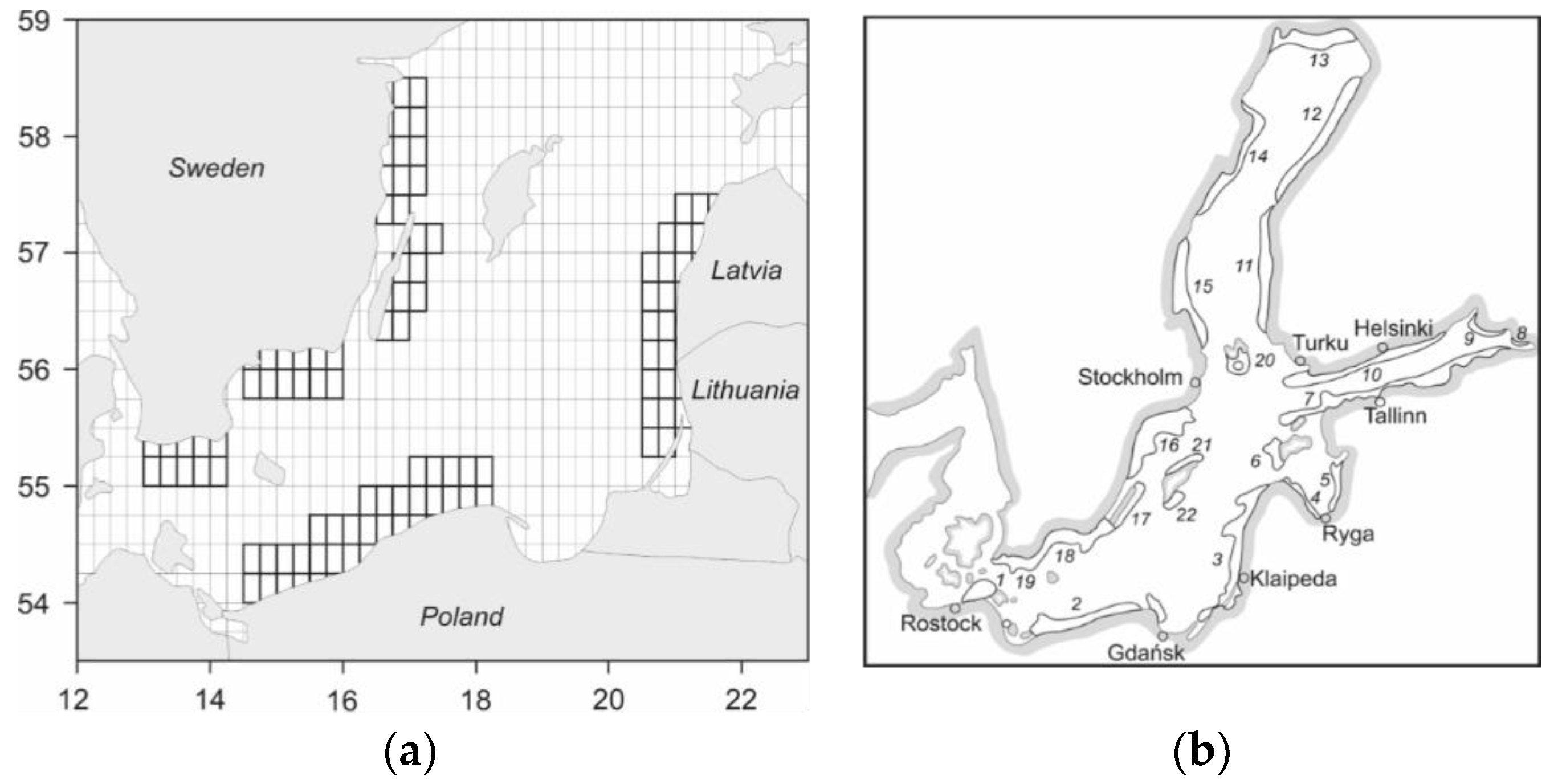
The area of the study encompasses the southern part of the Baltic Sea basin, and embodies several differently-oriented coastal zones. Upwelling regions considered in this study were chosen following Bychkova et al. [21], who delimited 22 areas of coastal upwelling occurrence in the entire Baltic Sea (Figure 1).

In the moderate climate zone, upwelling is best recognized in summer, when the strongest stratification is found, and warm surface waters overlay colder deeper water masses. Therefore only the summer months (June–August) were analyzed in this study. The mean daily sea surface temperature (SST) data available in the NOAA OI SST V2 High Resolution Dataset, provided by the NOAA/OAR/ESRL PSD, Boulder, Colorado, USA, (http://www.esrl.noaa.gov/psd) made the basis for the detection of upwelling cases [24]. This data has a relatively low temporal (1 day) and low spatial resolution (geographical grid 0.25° × 0.25°), which is disadvantageous in analyzing the upwelling cases. Nonetheless, the chosen dataset contains SST for over thirty years (1982–2017) and has no gaps, which is particularly important in climatological analysis. An alternative SST dataset of better resolution (0.03° × 0.03°), but of shorter period is available at: http://marine.copernicus.eu. The NOAA OI SST V2 High Resolution Dataset SST dataset was used in previous studies concerning upwelling along the Polish and Lithuanian-Latvian coasts [22,23]. Geographical resolution of 0.25° means 27.8 km resolution along the meridians and ca. 15–16 km resolution along the parallels. According to Lehmann et al. 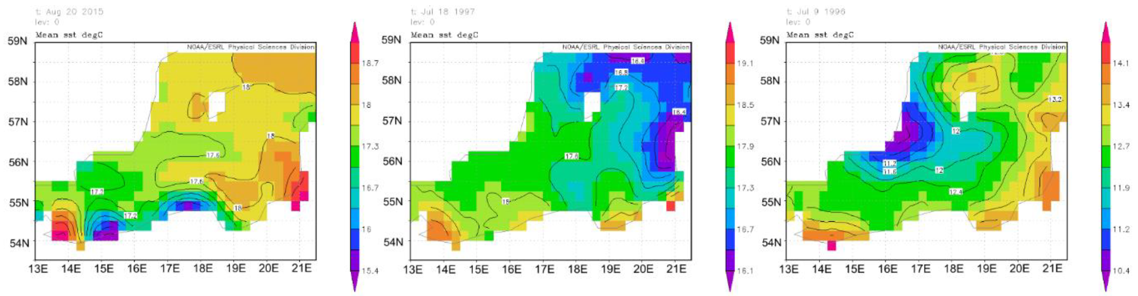[6] the horizontal scales of upwelling amounts to 10–20 km offshore and 100 km alongshore [13,21]. This asserts that the resolution of the SST data used in this study is sufficient to recognize upwelling events (examples in Figure 2). Nevertheless, one must remembered that smaller upwelling close to the coast may be undetectable using this NOAA OI SST data.

The two-steps procedure was undertaken to recognize the upwelling events. First, the pairs of grids along the coast were selected, and the SST differences between the grids closer to the coast and the farther ones were computed for each pair (see Figure 1a for the pixels engaged). A negative value indicated that the coastal waters were colder than open-sea waters, and an upwelling event probably took place. Secondly, maps of SST were plotted for each of the preliminary-selected days, and a visual detection method was applied to identify the phenomenon at each coastal region. Situations with a significant drop of SST along the coast, in comparison with the surrounding open waters, with SST isotherms bent towards the sea, were selected (examples in Figure 2). The seasonal (June–August) number of upwelling cases in each pixel indicated in Figure 1a was calculated providing a basis for further analysis.

For the atmospheric part of the analysis, monthly indices of macroscale circulation patterns were derived from the National Oceanic and Atmospheric Administration (NOAA) Climate Prediction Centre (CPC) datasets (ftp://ftp.cpc.ncep.noaa.gov/wd52dg/data/indices/nao_index.tim). 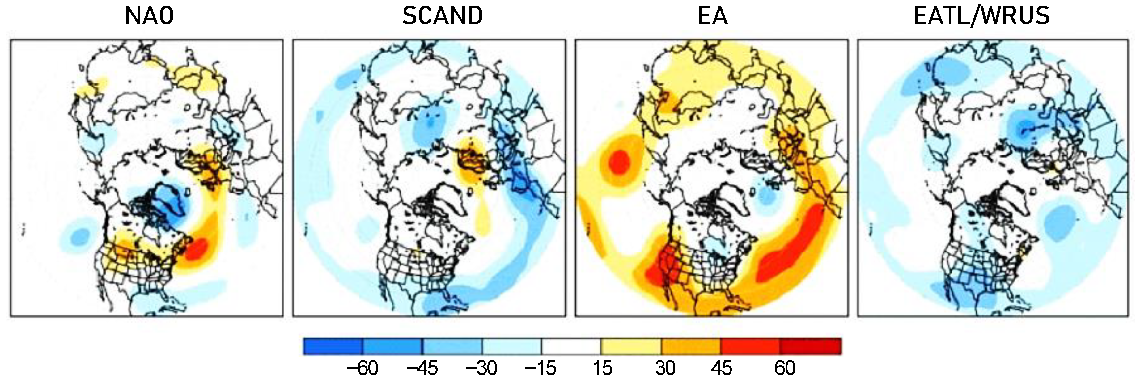These are PCA-based circulation patterns, and the principal component analysis (PCA) is applied to the Northern Hemisphere monthly mean standardized 500 hPa height anomalies [25]. Four teleconnection patterns are recognized as having the largest impact on climate and environment the Euro-Atlantic region (Figure 3). Among them the North Atlantic Oscillation (NAO) is regarded as the most prominent circulation pattern over the middle and high latitudes of the Northern Hemisphere. NAO is observed all over the year; however, its influence on the climatic conditions over the Euro-Atlantic region is most pronounced in winter. This is mainly because of the seasonal variation of the oscillation strength (it explains 36.7% of the variance of sea level pressure in winter, but only 22.1% in summer), and because of the seasonal changes in the spatial patterns of the NAO dipole center locations [25,26,27,28,29]. In summer both NAO centers are shifted northeast in comparison to the winter counterpart, which means that the summer southern dipole is located over northwestern Europe, rather than over the Azores–Spain region [27,28]. Regardless, not only winter but also summer fluctuations of the NAO phases and their intensity affect the weather and climate in Europe, mainly by modifying the direction and intensity of air circulation [28,29,30,31,32]. Therefore, NAO is likely to affect also the direction and magnitude of sea currents. The second teleconnection pattern included in the analysis is the Scandinavian (SCAND). It consists of a primary circulation center over Scandinavia, with weaker centers of opposite sign over western Europe and eastern Russia [25]. The positive phase of this pattern is associated with positive air pressure anomalies, sometimes reflecting major blocking anticyclones, over Scandinavia and north-western Russia. The East Atlantic (EA) pattern is considered as the second prominent mode of low-frequency variability over the North Atlantic. It is structurally similar to the NAO, and consists of a north-south dipole of anomaly centers, spanning the North Atlantic from east to west. The anomaly centers of the EA pattern are displaced southeastward to the NAO centers. The East Atlantic/ West Russia (EATL/WRUS) pattern is considered as the third prominent teleconnection pattern that affects Eurasia throughout year. The EATL/WRUS pattern consists of three main anomaly centers located over Euro-Atlantic region. The positive phase is associated with negative height anomalies located over the central North Atlantic and north of the Caspian Sea, and with positive height anomalies located over western Europe. However, the positive anomaly center in the positive phase is pronounced only in winter, and it weakens substantially in summer (Figure 3).

The Northern Hemisphere teleconnection patterns reflect the macroscale circulation conditions. In order to find out the local airflows and wind conditions, zonal (Z) and meridional (M) regional circulation indices were introduced in the atmospheric part of the analysis. To this end, the mean monthly sea level pressure (SLP) data was used. There are many sources of atmospheric data of different resolutions (for example the newest product ERA5 of 0.25° × 0.25° resolution, available at https://cds.climate.copernicus.eu). 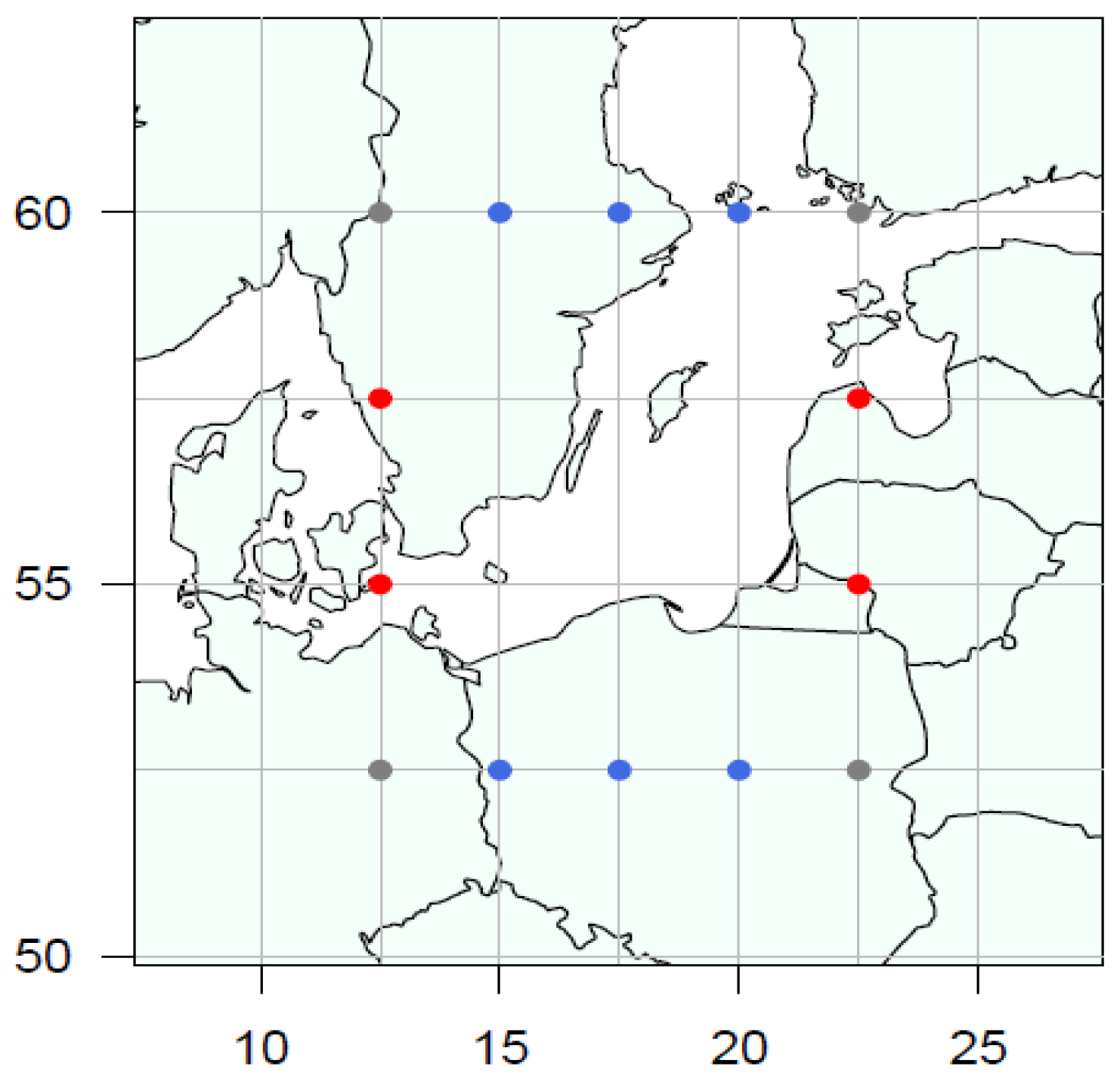However, in this study, for computing the common monthly circulation indices reanalysis (which was quite a simple task), data from National Centers for Environmental Prediction/National Centre for Atmospheric Research of spatial resolution 2.5° × 2.5° were fully sufficient [34]. 14 grids were used in the calculations and the monthly Z index was computed as a normalized difference between SLP at 52.5° N (SLP averaged for 5 grid points indicated in Figure 4) and 60° N (averaged, respectively) and M index as a normalized difference between 22.5° E (SLP averaged for 4 grid points) and 12.5° E (averaged, respectively). Positive values of Z/M indicated stronger than usual western/southern air-flow over the studied area. Lehmann et al. [20] constructed a similar local circulation index, called the Baltic Sea Index (BSI), using the normalized SLP anomalies at grid points 59.5° N, 10.5° E and 53.5° N, 14.5° E. They applied the BSI index to analyze the local atmospheric forcing on water circulation in the Baltic Sea.

Finally, anomalies of the coastal upwelling frequency in positive/negative phases of both macroscale and local circulation patterns were computed and plotted for each upwelling region. They were computed for each pixel separately according to the equation:

$$UFa=\frac{Up/n-U }{U}100\%$$

where: UFa—anomaly of upwelling frequency; Up/n—mean monthly number of cases of upwelling in the positive/negative phase of a given macroscale or local circulation pattern; U—mean monthly number of upwelling cases.

3. Results

3.1. Occurrence of Upwelling

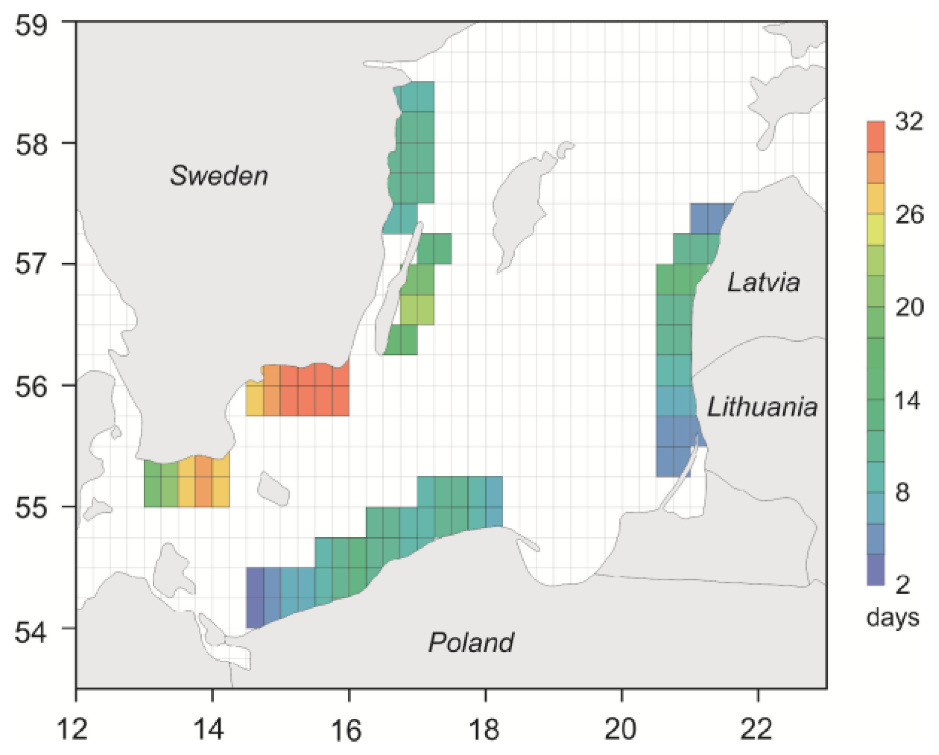
Within the southern Baltic Sea region the number of days with upwelling is diversified along the coastline, and is variable from year to year. The phenomenon is most frequent along the zonally oriented southern coasts of Sweden, where the mean number of upwelling events in the summer season (June–August) exceeds 30 days in several pixels (Figure 5). Nevertheless, the number of upwelling events along this part of the coast can exceed 50 days in a single summer season, like in the summers of 1990, 1998 and 2000, or even 60 days, like in 2015 and 2017. On the other hand, it may not exceed 10 days, like in the summers of 1982, 1995, 1996 and 2006.

Meridionally-oriented parts of the Swedish coast, including the eastern ridge of Oland island, experiences on the average 10–20 days with upwelling in a season, and again this number varies from above 40 days (in 1988, 2007, 2008, 2013, 2015, 2016, and 2017) to less than 5 days (in 1983, 1994, 1995, and 2003).

Coastal upwelling is least frequent along the Polish and Latvian-Lithuanian coasts, where the number of upwelling days rarely exceeds 10 (Figure 5). In fact, the phenomenon was not detected at all in several summer seasons, like in 1982, 1983, 1998, 1999, 2000 and 2012 along the Polish coast, and in 1985, 1987, 1991, 2007, 2011, 2012 and 2017 along the Latvian-Lithuanian coast. On the other hand, more than 30 days with upwelling were identified in 1992, 2002 and 2006 along the Polish coast, and in 1982, 1992, 1994, 1997 and 2006 along the Latvian-Lithuanian coast.

The mean seasonal number of upwellings indicates the regions that are predestined to frequent an occurrence of upwelling, while the year-to-year variability of its appearance and persistence suggests that the external–presumably atmospheric–conditions control the circulation of seawaters.

3.2. Impact of Macroscale Circulation Patterns on The Upwelling Frequency

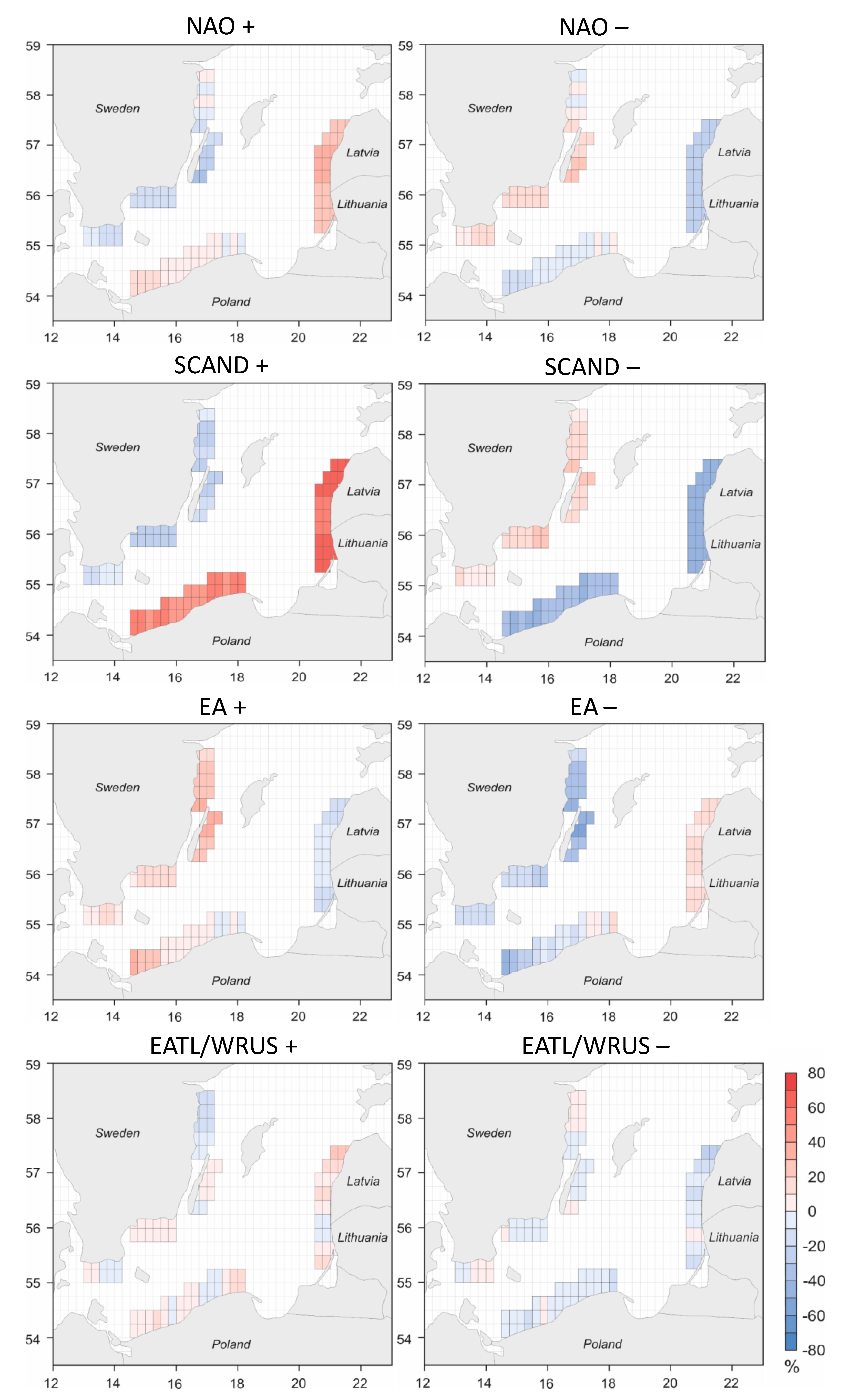
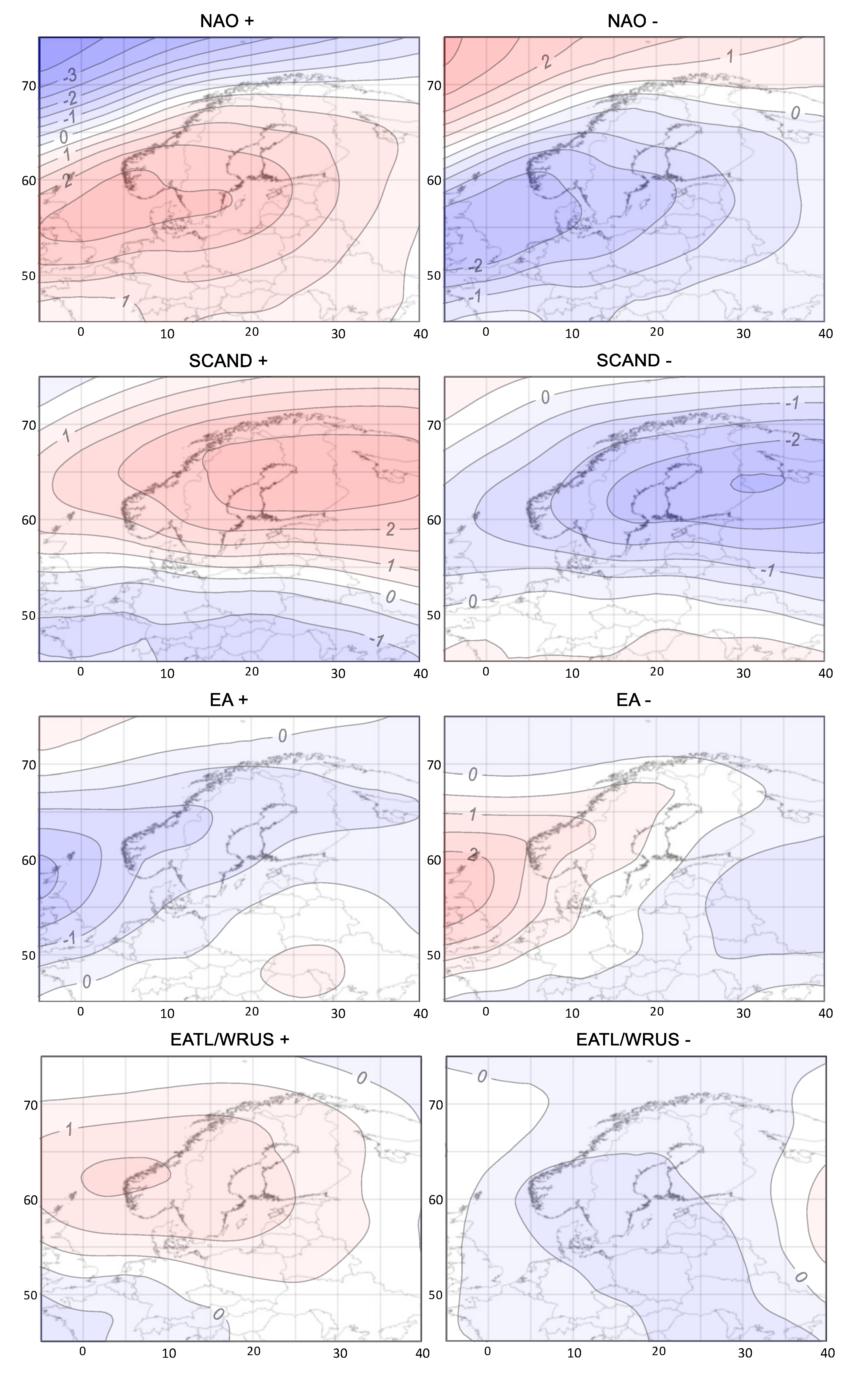
The NAO pattern, being commonly considered as the most prominent and recurrent circulation pattern over the middle and high latitudes of the Northern Hemisphere, particularly in winter, is strongly transformed in the summer. First of all, it is weaker than its winter counterpart and—which is crucial in this study—its southern center is shifted north- and east-wards. This means that the summer southern dipole is located over northwestern Europe, and encompasses the western part of the Baltic Sea (Figure A1). In the positive phase of NAO, in the westernmost part of the anticyclone, namely in the eastern part of the southern Baltic Sea basin, the northern airflow occurs, representing the gradient clockwise winds around the anticyclone. This enhances upwelling frequency along the eastern ridge of the southern Baltic, i.e., the Lithuanian-Latvian coast, by approximately 30% (Figure 6). A weak impact on the upwelling frequency both in positive and negative phases of NAO is observed in other coastal regions of the southern Baltic.

Among the macroscale teleconnection patterns considered in this study, the SCAND revealed the strongest influence on upwelling frequency. The positive phase of this pattern is associated with positive air pressure anomalies—sometimes reflecting blocking anticyclones—over Scandinavia (Figure A1). The anticyclone, accompanied with lower-than-normal pressure over western Europe and eastern Russia, induces geostrophic winds of clockwise direction around the high pressure center over Scandinavia. These bring about coast-parallel winds of eastern direction along the Polish coast and coast-perpendicular offshore winds at the Lithuanian-Latvian shore. These winds make favorable conditions for the rising of water along these coastlines, thereby causing upwelling. Consequently, the positive phase of the SCAND pattern exceeds the frequency of upwelling by more than 60% along the Lithuanian-Latvian coast and by more than 45–50% along the Polish coast (Figure 6, SCAND+). On the other hand, the pressure patterns affiliated with the positive phase of SCAND are inconvenient to upwelling along the entire Swedish coast, and they diminish the probability of its occurrence by approximately 20–30%. The opposite pressure pattern under the SCAND negative phase (lower than normal pressure over the Scandinavia) indicates the opposite distribution of upwelling frequency anomalies (SCAND– in Figure 6) with values exceeding −30 or even −40% along the Lithuanian-Latvian and Polish coasts.

The EA pattern is structurally similar to the NAO, but its dipole centers are displaced southeastwards to the NAO ones. This means that the air circulation over northern and central Europe in the positive EA phase has a significant south-western component (Figure A1). This enhances upwelling along the meridionally-oriented Swedish coast, and increases its frequency by approximately 20–30%. A southern air-flow component in the positive EA phase modifies the frequency of upwelling in the westernmost part of the Polish coast (increased by 20–30%), while it does not interfere in its central and eastern part.

The EATL/WRUS pattern, which in the positive phase characterizes with a weak center of positive SLP anomalies over southwest Scandinavia and the Norwegian Sea, does not reveal any significant impact on the frequency of coastal upwelling in the southern Baltic Sea basin.

3.3. Impact of Local Circulation Conditions on The Upwelling Frequency

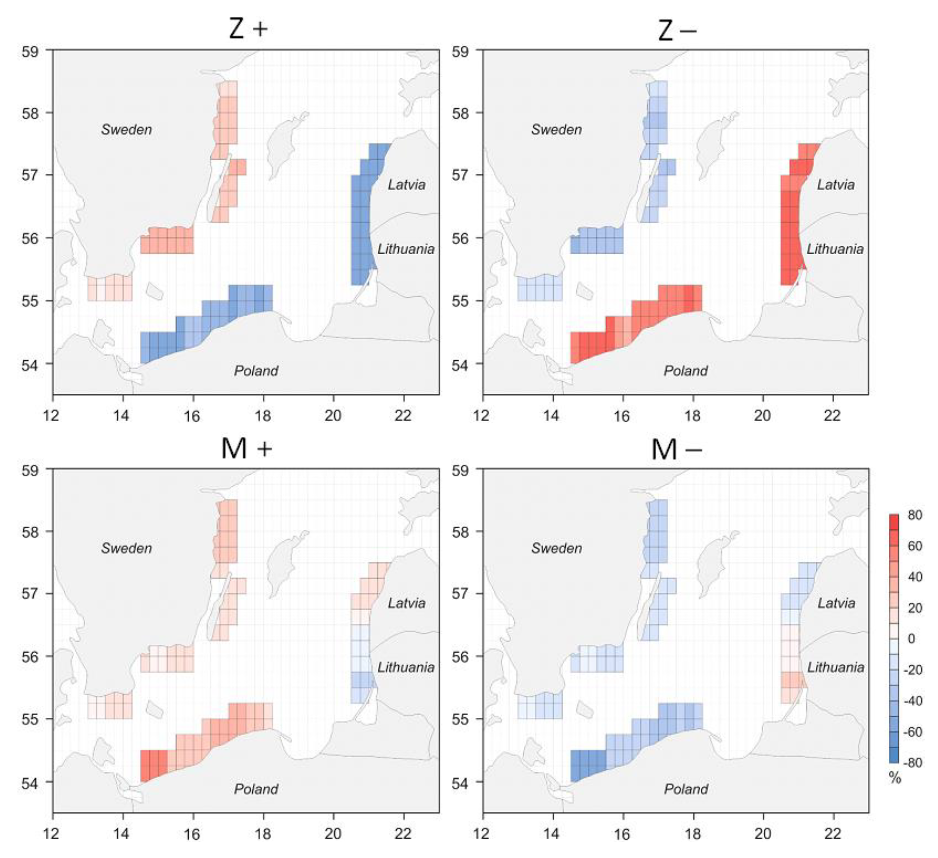
It was hypothesized that the local circulation patterns would better reflect the conditions which are favorable/unfavorable for coastal upwelling in the southern Baltic Sea basin. To this end zonal (Z) and meridional (M) regional circulation indices were introduced and anomalies of upwelling frequency were computed for positive/negative phases of Z and M. First, the correlations between macroscale and local circulation indices were computed. Statistically significant values were obtained for SCAND and Z as well as for EA and M (

Table 1. Pearson’s correlation coefficients between indices of the macroscale circulation patterns (North Atlantic Oscillation (NAO), Scandinavian (SCAND), East Atlantic (EA), East Atlantic/Western Russia (EATL/WRUS).) and local circulation indices (Z—zonal, M—meridional).

Circulation Patterns	NAO	SCAND	EA	EATL/WRUS
Z	−0.295	−0.767 **	0.204	−0.188
M	−0.328	−0.010	0.349 *	−0.038

* values statistically significant at p ≤ 0.05; ** values statistically significant at p ≤ 0.01.

). Strong negative correlation between SCAND and Z indices means that under the positive SCAND phase the anticyclonic conditions over Scandinavia substantially suppress westerly zonal airflow. Positive correlation between EA and M indices indicates significant southern air-flow component during the positive EA phase (Figure A1 and Figure A2). Local circulation indices are last related to the fourth macroscale circulation pattern, namely EATL/WRUS.

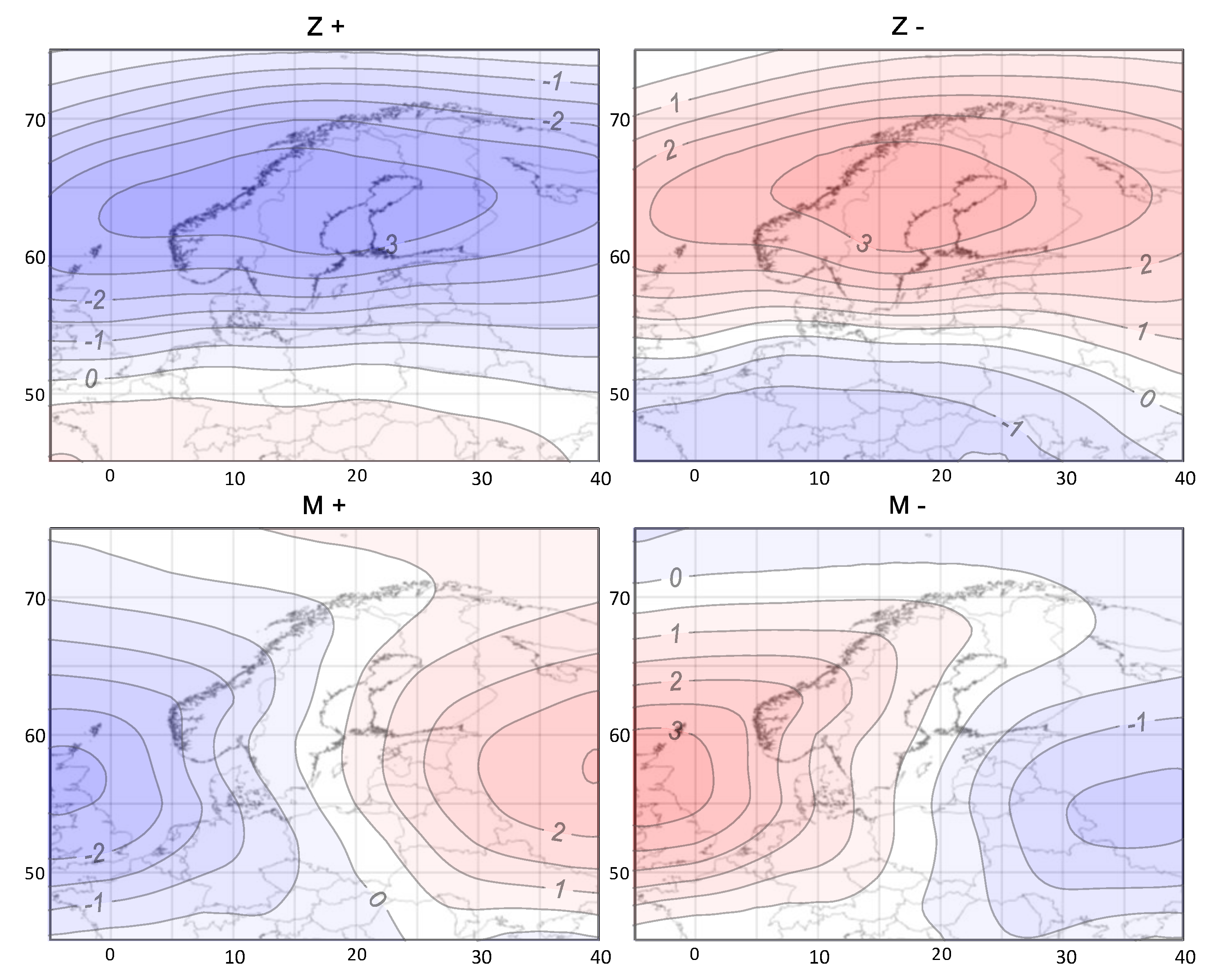
Local circulation pattern Z, being strongly correlated with SCAND, revealed a similar to SCAND spatial pattern of the upwelling frequency control. In the positive phase of Z, the amplified zonal western airflow suppresses the coastal upwelling in the southern and eastern parts of the southern Baltic Sea basin (Figure 7).

The frequency of upwelling is lowered by 50–65% along the Lithuanian-Latvian coast, and by 40–57% along the Polish coast. At the same time upwelling is slightly enhanced on the opposite side of the southern Baltic; i.e., upwelling frequency increases by up to 34% along the Swedish coast, where offshore and alongshore western winds blow. In the negative phase of Z, when the easterly airflow prevails, the opposite pattern of upwelling frequency is observed, namely there are much more-than-usually upwelling events along the Lithuanian-Latvian coast (increase by 58–76%) caused by the offshore winds, and along the Polish coast (40–67% more days with upwelling), caused by the eastern winds; at the same time the phenomenon is inhibited by 20–40% along the Swedish coast (Figure 7).

Meridional local-scale circulation has a weaker impact on the occurrence of upwelling within the southern Baltic Sea basin than the zonal one. In the positive phase of M, the intensified southern airflow and accompanying offshore winds enhance the upwelling frequency mainly along the Polish coast (by 20–30% in its central and eastern part, and by more than 50% in the westernmost part). Under the negative phase of M the frequency of upwelling along the Polish coast is substantially lowered. Some signals of changes in upwelling frequency, under the positive and negative phase of M, are observed also along the northern part of the Swedish coast (changes up to +30/−30% in the positive/negative M). In the other coastal regions only the weak influence of meridional airflow is recognized, which is expressed by the small changes in the upwelling frequency (0–20%) under the positive and negative phase of M.

4. Discussion

It was confirmed that within the southern basin of the Baltic Sea, coastal upwelling may occur almost constantly along the differently oriented coastlines, as almost each pressure pattern develop favorable conditions, i.e., alongshore blowing wind having the particular coast on its left or offshore winds blowing from the land interior. The number of days with upwelling is diversified along the coastline and extremely variable from year to year. The phenomenon is most frequent along the zonally oriented southern coasts of Sweden, where the average frequency of upwelling conditions exceeds 30%. A similar frequency of upwelling in these regions was proved by Lehmann et al. [6], and Myrberg and Andrejev [11]. However, they postulated a similarly high frequency for the Oland eastern coast as well, which was not reaffirmed in this study. Coastal upwelling is least frequent along the Lithuanian-Latvian and the Polish coast (up to 10%). Kowalewski and Ostrowski [17] emphasized that downwelling of the coastal waters is more frequent along the Polish coast due to the prevailing westerly winds [11].

The homogenous daily set of data used in this study allowed to evaluate the year-to-year variability of the upwelling occurrence. The frequency of upwelling may amount to over 60% of summer days along the Swedish coast, and may drop to 0% along the Polish and Latvian-Lithuanian coasts during single summer seasons.

This study’s results proved that both local and macroscale circulation patterns control the occurrence of coastal upwelling within the southern Baltic Sea basin. However, the impact strength varies, depending on the coastal region; the strongest relationships were found in the southeastern part of the basin, i.e., Polish and Lithuanian-Latvian coasts.

Among the macroscale circulation patterns, the SCAND appeared to have the strongest control of the horizontal flow of surface sea waters in the southern Baltic. The positive phase of SCAND is represented by a high pressure system located in the vicinity of the Baltic Sea, i.e., over Scandinavia. The clockwise air circulation around the Scandinavian anticyclone brings eastern flow over the southern Baltic Se basin which means coast-parallel winds along the southern coastline and offshore winds at eastern coastline, which—in line with Ekman’s theory—triggers upwelling [2]. The summer NAO, being weaker than its winter counterpart and, moreover, having its centers of action shifted to the northeast, appeared to have unexpectedly weak impact on upwelling occurrence. Some signals were found along the eastern Oland coast and southern Swedish coast, where the positive/negative phase enhanced/inhibited upwelling. An opposite reaction was found out along Lithuanian-Latvian coast. In the numerous previous studies NAO was proved to modify Baltic Sea conditions including ice extent, SST, surface currents, freshwater runoff, salinity and oxygen concentrations [20,35,36,37,38,39]. The relevance of NAO, however, seems to be definitely more substantial in winter than in summer, when the EA pattern (which is often described as a shifted southwards NAO) seems to be more important than NAO and it modifies the frequency of upwelling along the eastern Swedish coast. Not surprisingly, the fourth macroscale circulation pattern considered as relevant over Euro-Atlantic region—EATL/WRUS pattern reveals no impact on sea water circulation in the southern Baltic Sea basin.

Local circulation indices allowed to better recognize the atmospheric impact on upwelling frequency than the indices of the macroscale patterns. The anomalies in upwelling frequency are highest at positive/negative phase of the zonal circulation, identified at the regional pressure field. The Baltic Sea Index (BSI) similar to zonal local circulation used in this study was introduced by Lehmann et al. [20] in their research of atmospheric forcing on upwelling and sea water circulation in Baltic Sea. The BSI was computed as the difference of normalized SLP anomalies in two grid points located at about Szczecin (Poland) and Oslo (Norway). Authors proved that the positive BSI triggered inflow conditions in the Baltic Sea, and negative BSI values were correlated with outflow and a corresponding drop of the mean sea level. At the same time the correlation between the NAO and the volume exchange or mean sea level elevation of the Baltic Sea appeared to be small. Authors ascertained that possible relevance the NAO in the Baltic Sea region must first become evident in the local atmospheric conditions, which, furthermore, constitutes the direct impact [20]. It was reaffirmed in this study, that the local circulation patterns indicate the atmospheric forcing of coastal upwelling in the Baltic Sea better than the macroscale patterns. Among the latter, the SCAND was proved to have the strongest influence on upwelling frequency in summer, while the summer NAO revealed a weak relationship with the upwelling frequency.

Due to a strong fluctuation of pressure patterns in the Baltic Sea region and, consequently, large variability of circulation conditions, the analysis of the atmospheric forcing of coastal upwelling occurrence should be analyzed in different spatial scales. Furthermore, the future daily time-scale research should be carried out, which would allow to study the process of formation, persistence and disappearance of upwelling in reliance to fluctuations of atmospheric conditions.

5. Conclusions

Within the Baltic Sea, which is a small semi-enclosed basin with borders oriented in different directions, the coastal upwelling is considered to be a frequent phenomenon, as it may appear at some coast sections almost under any wind direction. The number of days with upwelling during the summer season (June-August) is diversified along the coastline and variable from year to year.

Both local and macroscale circulation patterns control the occurrence of coastal upwelling within the southern Baltic Sea basin. However, the impact strength varies, depending on the coastal region and the strongest relationships were found in the southeastern part of the basin, i.e., Polish and Latvian-Lithuanian coasts. Among the macroscale circulation patterns, the SCAND has the strongest impact on the horizontal flow of surface sea waters in the southern Baltic, which triggers upwelling. The summer NAO, appeared to have weak influence on upwelling occurrence, while the EA pattern (which is often described as a shifted southwards NAO) seems to be more important and modifies the frequency of upwelling along the eastern Swedish coast. Local circulation indices allow to recognize the atmospheric impact on upwelling frequency better than the indices of the macroscale patterns. The anomalies in upwelling frequency are highest at positive/negative phase of the zonal circulation, recognized at the regional sea level pressure field.