Article

Optimal Design of Air Quality Monitoring Network for Pollution Detection and Source Identification in Industrial Parks

1
Department of Environmental Science and Engineering, Fudan University, Shanghai 200438, China
2
Big Data Institute for Carbon Emission and Environmental Pollution, Fudan University, Shanghai 200433, China
3
Shanghai Institute of Eco-Chongming (SIEC), No.3663 Northern Zhongshan Road, Shanghai 200062, China
*
Author to whom correspondence should be addressed.
Atmosphere 2019, 10(6), 318; https://doi.org/10.3390/atmos10060318
Submission received: 11 May 2019 / Revised: 29 May 2019 / Accepted: 4 June 2019 / Published: 11 June 2019
(This article belongs to the Section Air Quality)

Abstract

:
Dense air quality monitoring network (AQMN) is one of main ways to surveil industrial air pollution. This paper is concerned with the design of a dense AQMN for H2S for a chemical industrial park in Shanghai, China. An indicator (Surveillance Efficiency, SE) for the long-term performance of AQMN was constructed by averaging pollution detection efficiency (rd) and source identification efficiency (rb). A ranking method was developed by combing Gaussian puff model and Source area analysis for improving calculation efficiency. Candidate combinations with highest score were given priority in the selection of next site. Two existing monitors were suggested to relocate to the west and southwest of this park. SE of optimized AQMN increased quickly with monitor number, and then the growth trend started to flatten when the number reached about 60. The highest SE occurred when the number reached 110. Optimal schemes of AQMNs were suggested which can achieve about 98% of the highest SE, while using only about 60 monitors. Finally, the reason why the highest SE is less than 1 and the variation characteristics of rd and rb were discussed. Overall, the proposed method is an effective tool for designing AQMN with optimal SE in industrial parks.

1. Introduction

Dense air quality monitoring stations have been considered one of the main ways to surveil air pollution in industrial parks. Compared with mobile equipment, a dense fixed network can ensure daily surveillance coverage. Thus, designing a proper dense air quality monitoring network (AQMN) with optimal surveillance performance is crucial for the management and control of air pollution in industrial parks.
Optimal design of AQMN has been widely investigated in the literature [1,2,3,4,5,6,7,8,9,10,11]. It can be considered as an optimization problem searching for the best combination of the location and number of candidate monitors. The AQMN arrangement is determined by different design criteria such as environmental, social, and economic objectives and the monitoring costs [4,12,13]. Many heuristic algorithms have been applied to solve the optimization problem for AQMN design at different scales [6,8,11,14,15]. For example, Henriquez et al. in [15] employed a variational approach to compare the results of an optimal arrangement with the current AQMN for Santiago, Chile. Benis et al. in [8] designed a sensitive AQMN based on Ant Colony Optimization (ACO) and Genetic Algorithm (GA) respectively for an industrial district. Considering the capability of quick diagnosis of pollution episodes, the sensitivity of potential locations to sources was considered as a design objective as well as the coverage area and violation over ambient standards. Hao and Xie in [11] performed an optimal redistribution of an urban AQMN for SO2 and NO2 in Shijiazhuang city using the WRF-CALPUFF model and non-dominated sorting GA. The maximization of coverage with minimum overlap and the ability to detect violations of standards were considered as the design objectives. Gupta et al. in [16] developed a systematical method by combing Land use regression (LUR) and Spatial annealing simulating (SSA) to place AQMN for decreasing the spatial mean predictor error in highly- populated spaces. However, few have focused on the source reconstruction performance of AQMN in optimal design. Recently, many studies in the literature have explored how to reconstruct source characteristics based on the measurements from a dense AQMN and have analyzed the influence of the AQMN distribution on the back-calculation [17,18,19,20], while only single emission episodes were considered as the concerned objectives in these studies.
In our previous study, the long-term performances of a boundary-type AQMN planning program for pollution detection and source identification for H2S in a chemical industrial park were evaluated [21] respectively. There were two existing stations in the industrial park concerned, which were located at the west-southwest and south-southwest of this park. In the evaluation, only single source located in the center of this park was considered as the real source and ten remaining suspected source were considered as fake sources, considering that they may disturb the reconstruction of the real source in this park. Added monitors were prioritized to be placed at the downwind orientations with higher meteorological frequency. The annual efficiency of pollution detection could reach 100% when sixteen monitors were placed downwind corresponding to sixteen wind directions, while the results of annual source identification efficiency showed that two fake sources on average among ten sources may disturb the identification of the real source. Thus, it was suggested to deploy more monitors inside the industrial park to further improve the source identification efficiency.
Optimization of a dense AQMN was further investigated for the above chemical industrial park in this article. The AQMN, distributed densely, aims to improve the source identification performance for this park. The long-term surveillance (i.e., pollution detection and source identification) performance of the AQMN for air pollution episodes in industrial parks was considered as a composite design indicator for the comparison among different candidate schemes. The disturbance characteristics vary with the meteorological conditions, meanwhile the surveillance performances for different real sources in this park are different and needs to be considered comprehensively for obtaining an optimal scheme. Thus, optimization of the surveillance efficiency (SE) under long-term meteorological conditions and the existence of multiple sources were considered in the dense AQMN design. Meanwhile, the candidate locations of monitors were selected from the non-productive area of the industrial park instead of only the above boundary-type planning program. It is difficult to carry out direct sampling calculations for such a large number of candidate points. A ranking strategy for candidate combinations of monitors based on their SE performance was designed for excluding invalid points to improve calculation efficiency. Candidate combinations with higher scores were given priority in the selection of the next added sites.
The dispersion model and back-calculation method used in our previous study were also employed here for the evaluation of the SE for AQMN optimization. Ambient concentration data were replaced by simulated concentrations generated by the dispersion model. Different types of dispersion models such as Gaussian plume model, Gaussian puff model, Lagrangian stochastic model, and computational fluid dynamics [20,22,23,24,25,26,27,28,29,30,31] can be used for simulating dispersion in pollution detection and source reconstruction. The Gaussian puff model was employed here instead of a refined method to reproduce the spatial and temporal variations of H2S concentrations for the studied industrial park because emission sources arranged densely and accurate environmental conditions are always difficult to obtain for a refined simulation using a model. Meanwhile, sufficient information on source terms is difficult to capture in real episodes, especially for some unexpected, short-term, and intermittent emissions. Such information will further increase the error of the refined simulation. Single pollution episode would be captured once there was one monitor covered by the simulated envelope.
The collection of potential source locations for source identification was obtained based on the result back-calculated by the source area analysis method (described in [32]). Source area analysis method is an insightful way to reconstruct source terms with limited or sufficiently many monitors. Number of suspected sources covered by the back-calculated source area was further counted for the following statistics relating to the source identification efficiency.
The framework of this article is organized as follows. In Section 2, after a brief description of the data configuration, the SE indicator, Gaussian puff model (for the simulation of the concentration variations), and source area analysis (for the reconstruction of source terms) are presented. In Section 3, two existing monitors are evaluated and redistributed, then the design schemes for three scenarios are provided and analyzed. In Section 4, the conclusions and suggestions are given.

2. Methods

2.1. Data Configuration

A chemical industrial park in Shanghai, China was concerned. H2S was considered as the intended pollutant for surveillance. It is a common odor pollutant in industrial parks, especially in chemical parks. Abnormal emission episodes caused by such an odor pollutant are irregular and with high uncertainty. This industrial park covers an area of approximately 19 km2. There were eleven sources of H2S in this park, as shown in Figure 1. The two existing monitoring sites (M1 and M2) in Figure 1 were located to the west-southwest and south-southwest of this park. The non-productive area in this park was meshed with a grid interval of 100 m and 1221 candidate sites were identified (Figure 1). The lower detection limit was set to 0.56 μg m−3 [33], and the background concentration was 13.0 μg m−3.
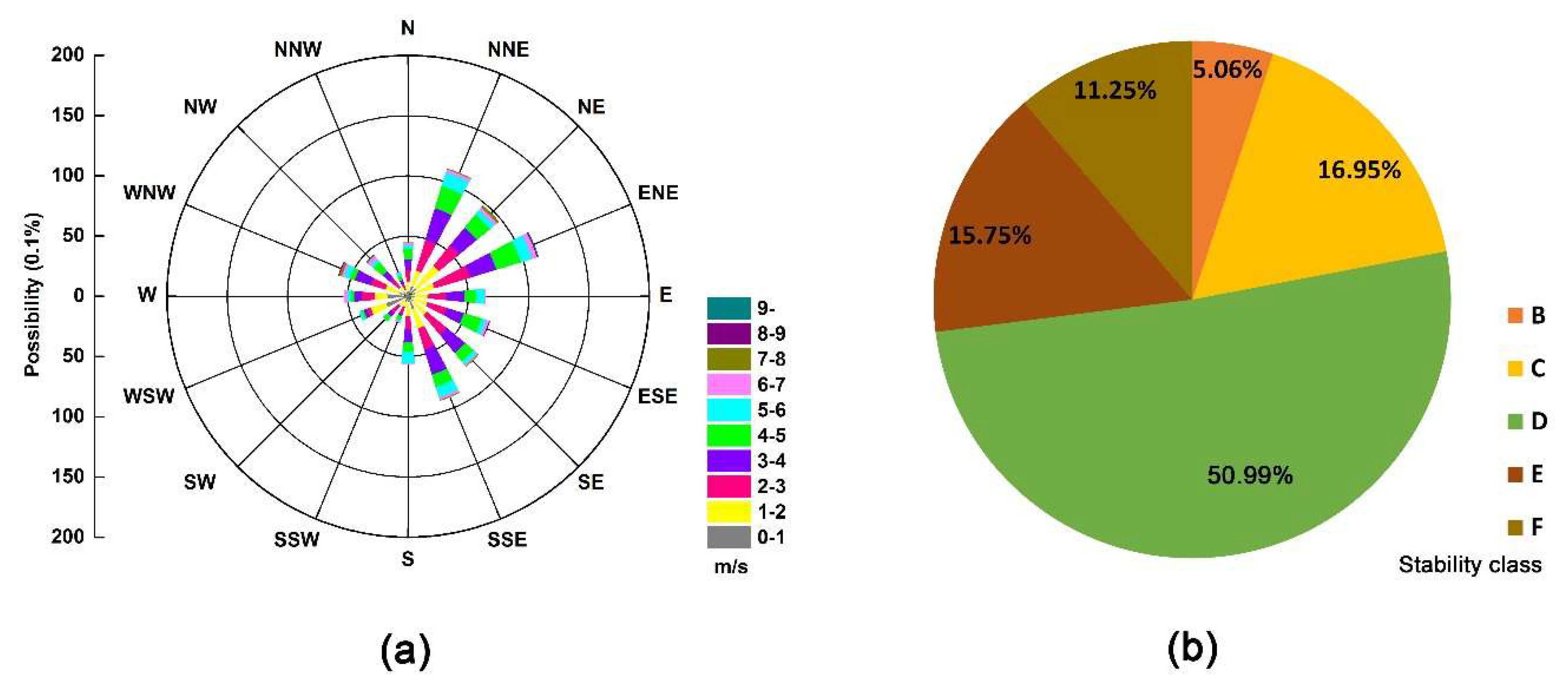
Whole-year meteorological measurements at a temporal resolution of one hour were used in the study (Figure 2), considering that one year is the minimum period required to represent the meteorological fluctuations of a study area normally [34]. The annual frequencies of the sixteen wind directions ranged from 2.18% to 11.32%. The prevailing wind directions, the north-northeast, northeast, and east-northeast, had a total frequency of approximately 32.21%. The north-northwest wind frequency was the lowest, accounting for only 2.18%.
Wind speeds were classified into two levels: low wind conditions (0.5–2.0 m s−1) and non-low wind conditions (2.0–10.0 m s−1). The mean wind speed was 3.49 m s−1, and the low wind frequency was 11.74%. The frequency of calm wind conditions was 2.94%. 1.0 m s−1 and 2.0 m s−1 were selected to represent low wind conditions and non-low wind conditions respectively, considering the similar results with wind speeds of 2.0–10.0 m s−1. Neutral stability accounted for approximately 50.98% of the whole-year atmospheric conditions.

2.2. Method

2.2.1. Gaussian Puff Model

Detailed concentration distributions and temporal variations of H2S for pollution detection and source identification were given by the Gaussian puff model, referring to the guideline models for environmental risk assessment on projects [35,36]. The simulated concentration measurement C is provided as follows:
C i ( x , y , z , t ) = Q i ( 2 π ) 3 / 2 σ x σ y σ z e x p [ ( x x i ) 2 2 σ x 2 ] e x p [ ( y y i ) 2 2 σ y 2 ] { e x p [ ( z z i ) 2 2 σ z 2 ] + e x p [ ( z + z i ) 2 2 σ z 2 ] }   ,
where Ci is the predicted concentration of the pollutant at the point (x, y, z) from puff i at (xi, yi, zi); t is the release time; Qi is the emission strength of the puff; zi is the effective stack height of the puff centreline; and σx, σy, and σz represent the dispersion coefficients of the concentration distribution in the horizontal, crosswind, and vertical directions, respectively. The calculation of the dispersion coefficients were completed according to MEEPRC in [37].
For the forward simulation, the emission rate was set to approximately 100 kg h−1. Real observations of wind speed and wind direction were adopted, and atmospheric stability classifications could be ascertained through the temperature gradient wind speed method (∆T/U) [34]. The temperature gradients could be acquired with the help of the sounding data from the Shanghai International Exchange Station (No. 58362), supported by university of Wyoming (http://weather.uwyo.edu/upperair/sounding.html, Site) [38].

2.2.2. Source Area Analysis

The source area analysis method established in our previous paper [32] was employed to perform the source identification. It provides an approach to obtain the source area by means of meteorological data and concentration measurements. First, the computation domain is meshed, and the centre of each grid cell is treated as a point emission source. In addition, a reasonable space is provided for each remaining source parameter (such as emission rate, start time and source height). Then, optimal combinations are searched from these spaces at each point. The concentration prediction error at the monitor is evaluated for the searched combinations. A combination of source parameters is considered feasible provided the calculated concentration prediction error is less than the defined error limit. The grid point is accepted as long as a feasible combination is obtained. Finally, the source area is obtained based on the optimal err values of all grid points.
In our back-calculation, the study area was meshed with a grid interval of 100 m. The upper limit of the release rate was 360 kg h−1 in the back-calculation, which was back-calculated based on the peak concentration throughout the whole year at monitors. The emission time was set to be no more than four hours before the detection time.
The prediction error for each combination of source parameters at each point is calculated using the following equation:
e r r = 10 | log C s C m |
where Cs and Cm are the simulated and measured concentrations, respectively.
The prediction error in Equation (2) represents the composite level of multiple errors (i.e., measurement error, modelling error, sampling error, source term error and others). These errors are difficult to separate in practice. Considering that the sampling and measurement errors are usually involved in the assessment of the modelling error, the prediction error limit was directly represented by the modelling error of the above dispersion model. The error limit was set to a factor of a to reflect a match between the measured and simulated concentrations in this paper [39].

2.2.3. The SE Indicator

The AQMN design is the process of solving an optimization problem with regard to SE, which is defined to indicate the averaging score of pollution detection and source identification efficiency, as shown in Equation (3):
S E = k 1 r b + k 2 r d ( k 1 + k 2   = 1 ) ,
where the parameters k1 and k2 are used to weight the importance of pollution detection and source identification in the surveillance, respectively. k1 was equal to k2 in this paper.
Each source was considered as the real source of concern in the calculation and assumed to be a continuous emitter throughout the whole year, meanwhile other sources were considered as fake sources. Synthetic concentrations at monitors were obtained for each real source by the Gaussian puff dispersion model. A record whose concentration exceeded the upper limit was defined as a pollution episode. The envelope profiles plotted based on measurements were overlaid with the monitor arrangements to identify whether a single pollution episode was detected by given monitors. Source area for single pollution episode were determined by the Source area analysis method. The back-calculated source area profile was overlaid with the suspected source arrangements to identify whether each suspected source was covered by given source area.
The efficiency of pollution detection (rd) is defined to indicate the average of the annual accumulative probability of detecting violations where the record’s concentrations are over the air quality ambient standards for each real source emission, as shown in Equation (4):
r d   =   e = 1 E ω e i   =   1 I r d , e , i
r d , e , i   =   m = 1 M P m T m , e , i
where rd,e,i represents the annual accumulative probability of detecting violations from real emission source e for a single monitor i; ω e represents the weight of each real source; Pm represents the frequency of meteorological scenario m; Tm,e,i stands for a probability of the violation from real emission source e is captured by monitor i under meteorological scenario m (Tm,e,i = 1 means the violation is captured and Tm,e,i = 0 otherwise); M is the total number of meteorological scenarios; and E and I are the total numbers of emission sources and monitors, respectively.
The efficiency of source identification (rb) is the average of the annual accumulative probability of the number performance of suspected sources in the back-calculated source area for each real source emission in the industrial park. This is formulated as Equation (6).
r b   =   e = 1 E ω e r b , e ,
r b , e   =   m   =   1 M P m V m , e ,
V m , e   = 1 s = 1 S N m , e , s   ,
where r b , e is the efficiency of source identification when the real emission source is e; ω e represents the weight of each real source; Pm is the frequency of meteorological scenario m; V m , e represent the number performance of suspected sources covered by the back-calculated source area under meteorological scenario m when the real emission source is e. Nm,e,s is used to make a judgement as to whether fake source s is located in the source area under meteorological scenario m when the real emission source is e, such that Nm,e,s = 1 if the violation is captured and fake source s is located in the source area, and Nm,e,s = 0 otherwise; M is the total number of meteorological scenarios; and S is the total number of suspected sources in the industrial park. Only a single source was considered as the real source for each simulation, and the other sources were considered as fake sources.

2.2.4. Optimal Design of the AQMN

In this work, a design model for AQMN optimization was constructed based on the indicator SE. It consists of three sub-modules considering different characteristics of existing and added monitors in actual application scenarios.
  • Scenario I: Existing sites are fixed and more sites with a known number are added based on the performance of existing sites;
  • Scenario II: Existing sites are fixed and more sites with an unknown number are added based on the performance of existing sites;
  • Scenario III: Existing sites are allowed to be relocated and more sites with an unknown number are added.
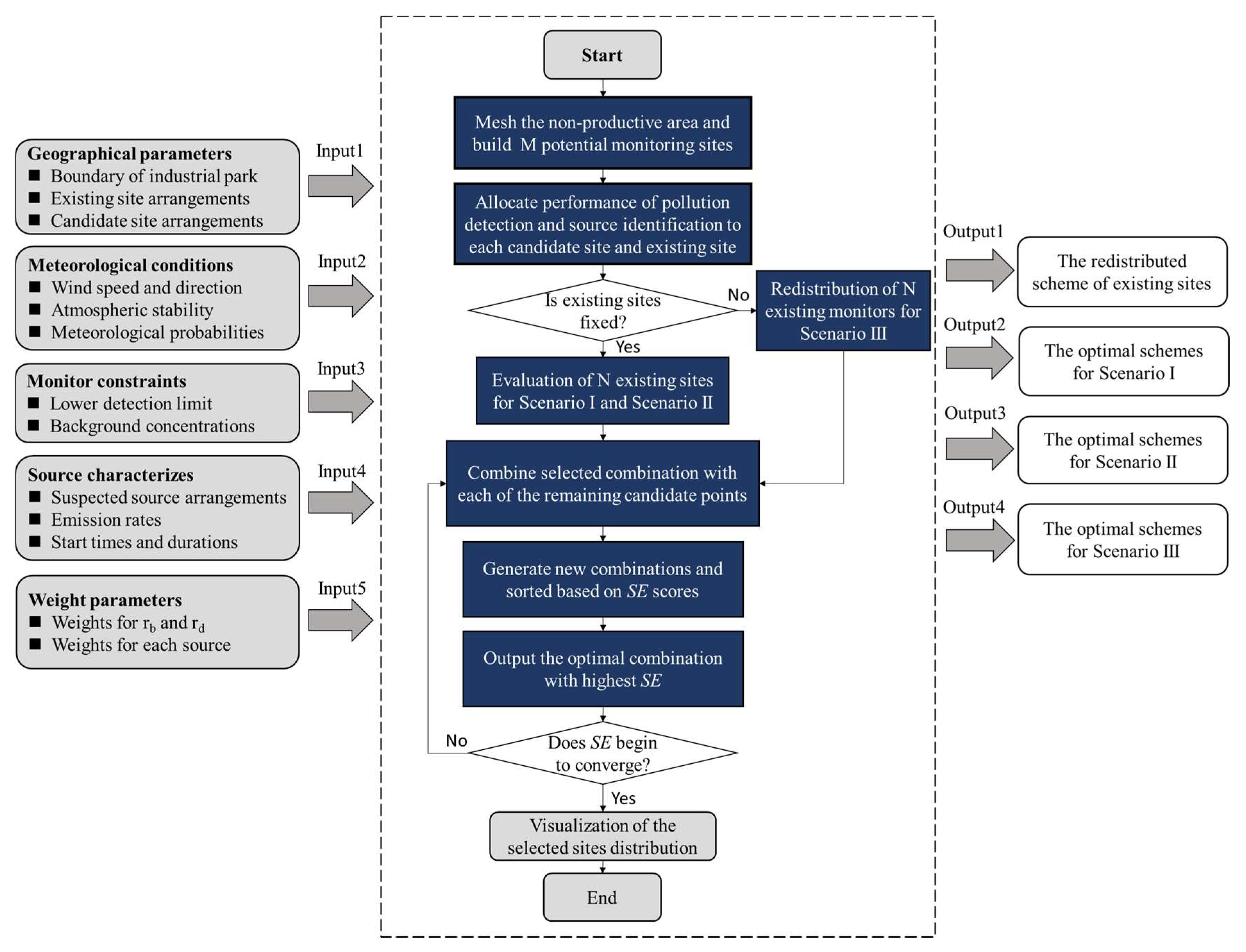
The flowchart of the optimization process is shown in Figure 3. It can be broken down into the following steps:
  • Step 1. The industrial park is divided into M grids and the centroid of each grid cell is considered as a potential monitoring site;
  • Step 2. Concentration results obtained by Gaussian puff dispersion and source area results back-calculated by source area analysis are allocated to corresponding grid cells for each meteorological condition when each source is considered as the real emission source;
  • Step 3. The SE scores of integrated existing sites are evaluated. If existing AQMN with the N sites are fixed (Scenario I and Scenario II), continue the next step; while if existing N sites are allowed to be relocated (Scenario III), site combinations with the same number are generated from M candidate sites and evaluated. Then sorted based on their SE scores, and the combination with highest score is considered as the optimal redistribution scheme;
  • Step 4. The selected existing or redistributed combination with N sites is further combined with each of the remaining candidate points. The new combinations with N + 1 are generated and evaluated, then sorted again based on their scores, and the N + 1 combination with highest score is considered as the optimal selection when one added monitor is available;
  • Step 5. The optimal N + 1 selection is further combined with each of the remaining candidate points. The new combinations with N + 2 sites are generated and evaluated, then these combinations are sorted again based on their scores, and the N + 2 combination with highest score is considered as the optimal selection when two added monitors are available;
  • Step 6. This process is continued until the number of selected sites is adequate (for Scenario I) or the surveillance efficiency begin to converge (for Scenario II and Scenario III).

3. Results

3.1. Evaluation of Existing Monitors

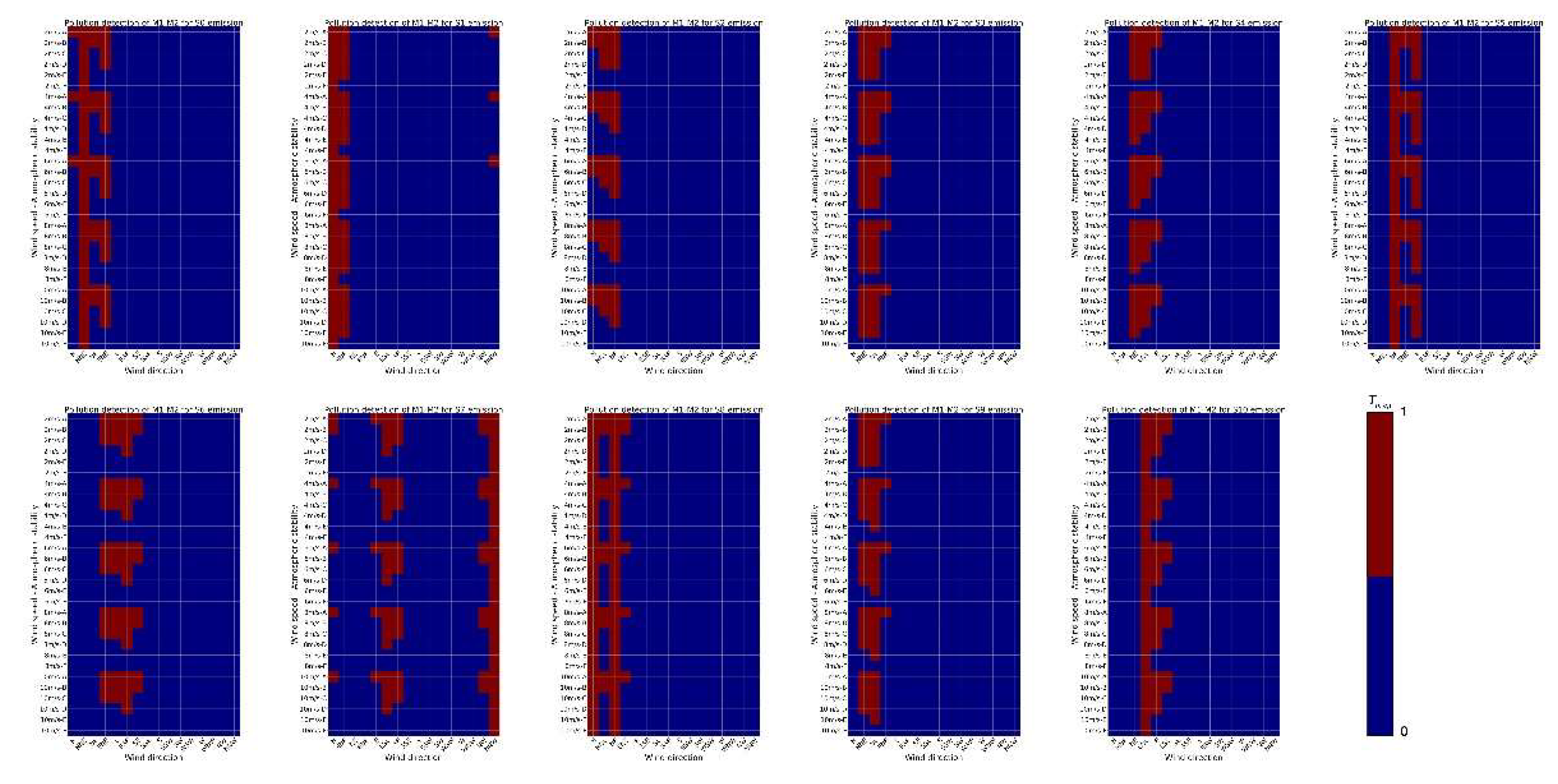
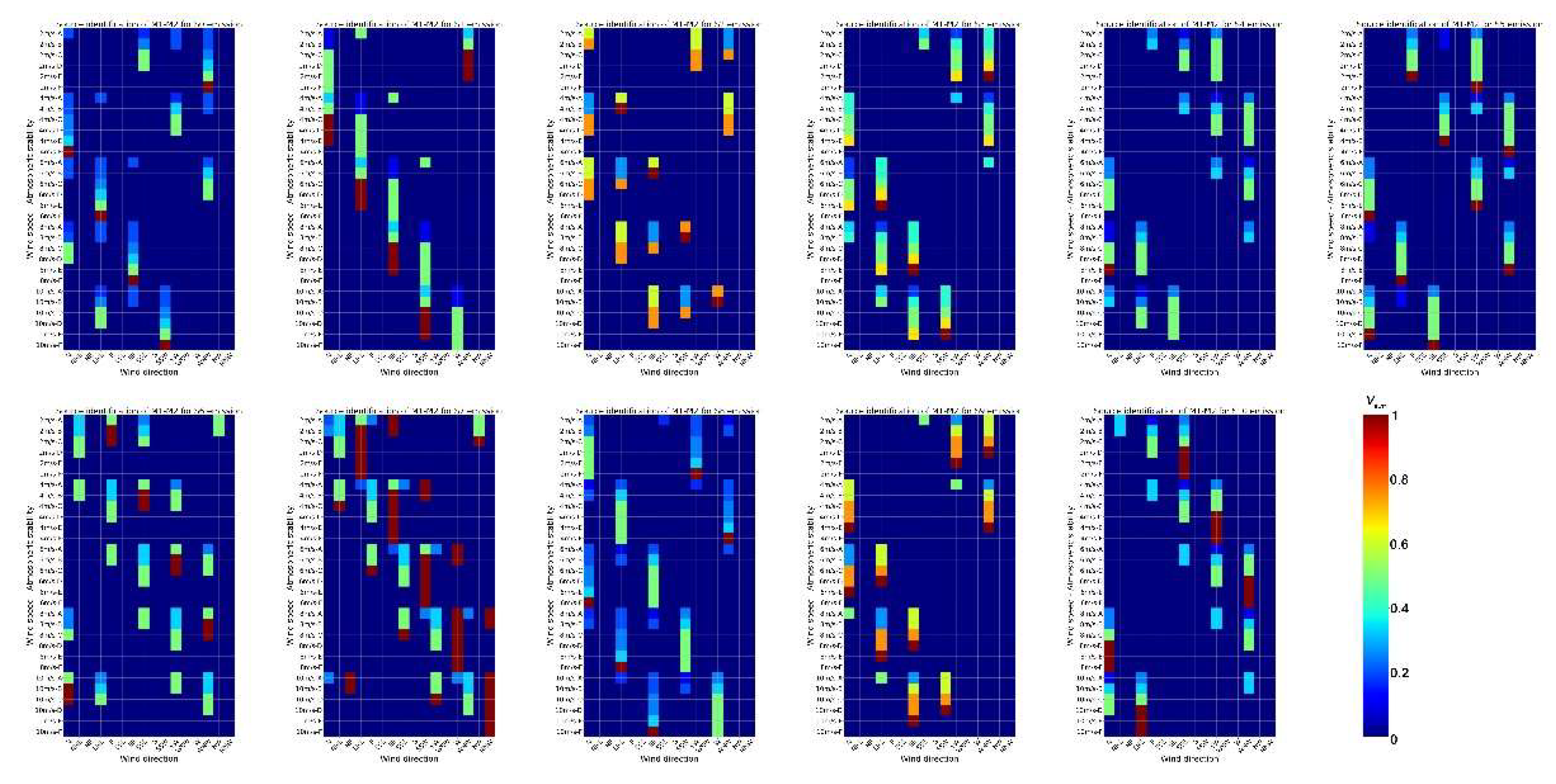
The score performance of the two existing monitors is illustrated in Table 1. The SE score of integrated M1 and M2 was 0.109 as shown in Table 1, where rd and rb were 0.146 and 0.072 respectively. This was still insufficient for this developing industrial park. Tm,e,i and Ve,m performances of integrated M1 and M2 for different source emissions under different meteorological conditions were presented in Figure A1 and Figure A2 (Appendix A) respectively. Noted that the sum of the individual rd scores of the two existing monitors was slightly higher than the integrated score of them, while the rb scores of them were equal. This is because the two monitors may be covered simultaneously by the envelope for a single pollution episode under the low wind condition, while the source area back-calculated based on integrated measurements always covered the eleven sources as well as that based on the individual measurements. More discussion about variations of dispersion envelops and back-calculated source area characteristics with meteorological conditions have been provided by Huang et al. [21].
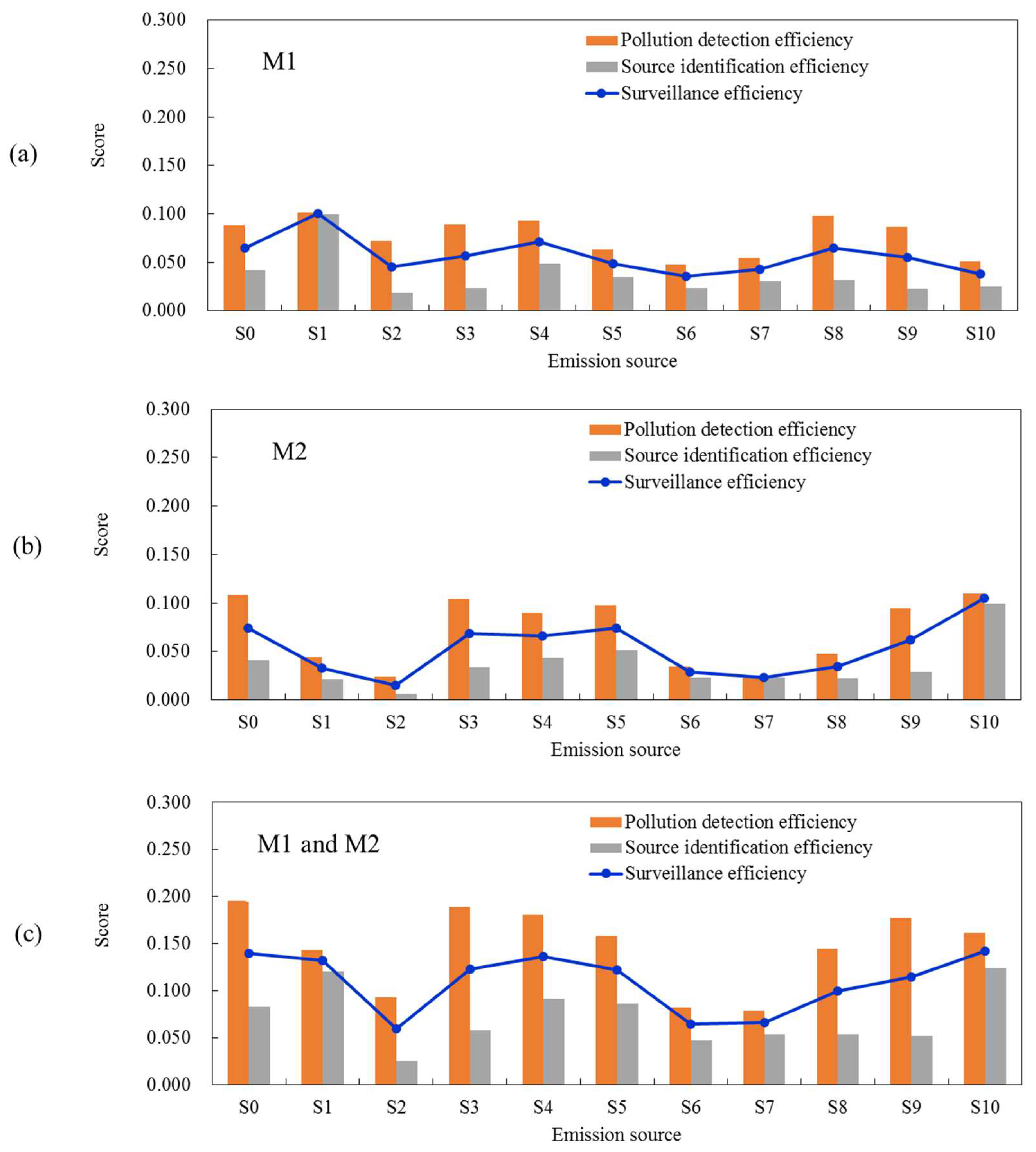
Further, the individual and integrated performances of M1 and M2 for different real emission sources are presented in Figure 4. There were nearly significant differences in SE between M1 and M2 (Table 1), while there were obviously significant differences for different real emission sources. For example, the SE of M1 located at the west-southwest of this park is 0.100 when S1 is considered as the real source, which is the highest score among these sources. M2 located at the south—southwest only presents an SE score of 0.032 in the same situation. However, the SE of M2 is 0.105 when S10 is considered as the real source, while the SE of M1 is 0.038.
The SE score for S0 located in the centre of this park was about 0.147 in the integrated performance of M1 and M2. This is the highest score among the eleven sources because the rb score for S0 was higher than those for the other sources. However, the SE scores for S2, S6, and S7 were obviously lower than those for other sources. In particular, the SE score of the integrated performance for S2 located in the north of this park was only 0.059, which was the lowest score. This is because its rd was only 0.026, obviously lower than those of other sources.

3.2. Optimal Schemes of AQMN for Different Scenarios

In this section, the design was implemented to obtain the optimal schemes for three application scenarios. In Scenario I, the number of added monitors was known and two existing monitors (M1 and M2) were fixed, while the number of added monitors was unknown in Scenario II. Further two existing monitors were considered to do the redistribution in Scenario III.

3.2.1. Scenario I

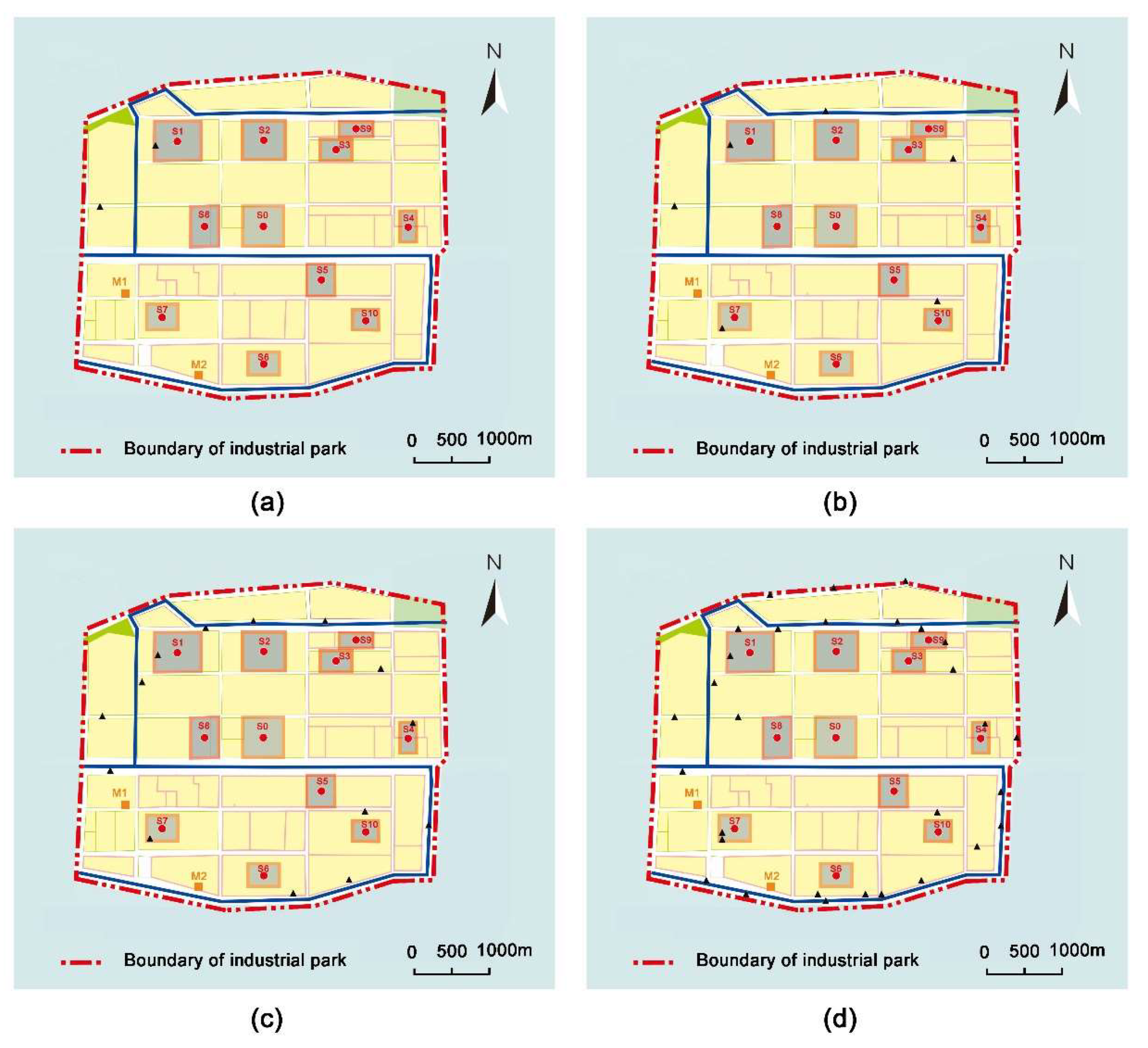
Two existing monitors were fixed and the numbers of added monitors were 2, 6, 14, and 30. The optimal schemes with the different numbers of monitors are illustrated in Figure 5. The results showed that the optimal distribution of the AQMN was arranged almost at the boundary of this park when the number of added monitors is limited. Locations downwind of wind directions with high frequencies were still preferred because effective pollution detection may then be ensured, which is also the premise of effective back-calculation.
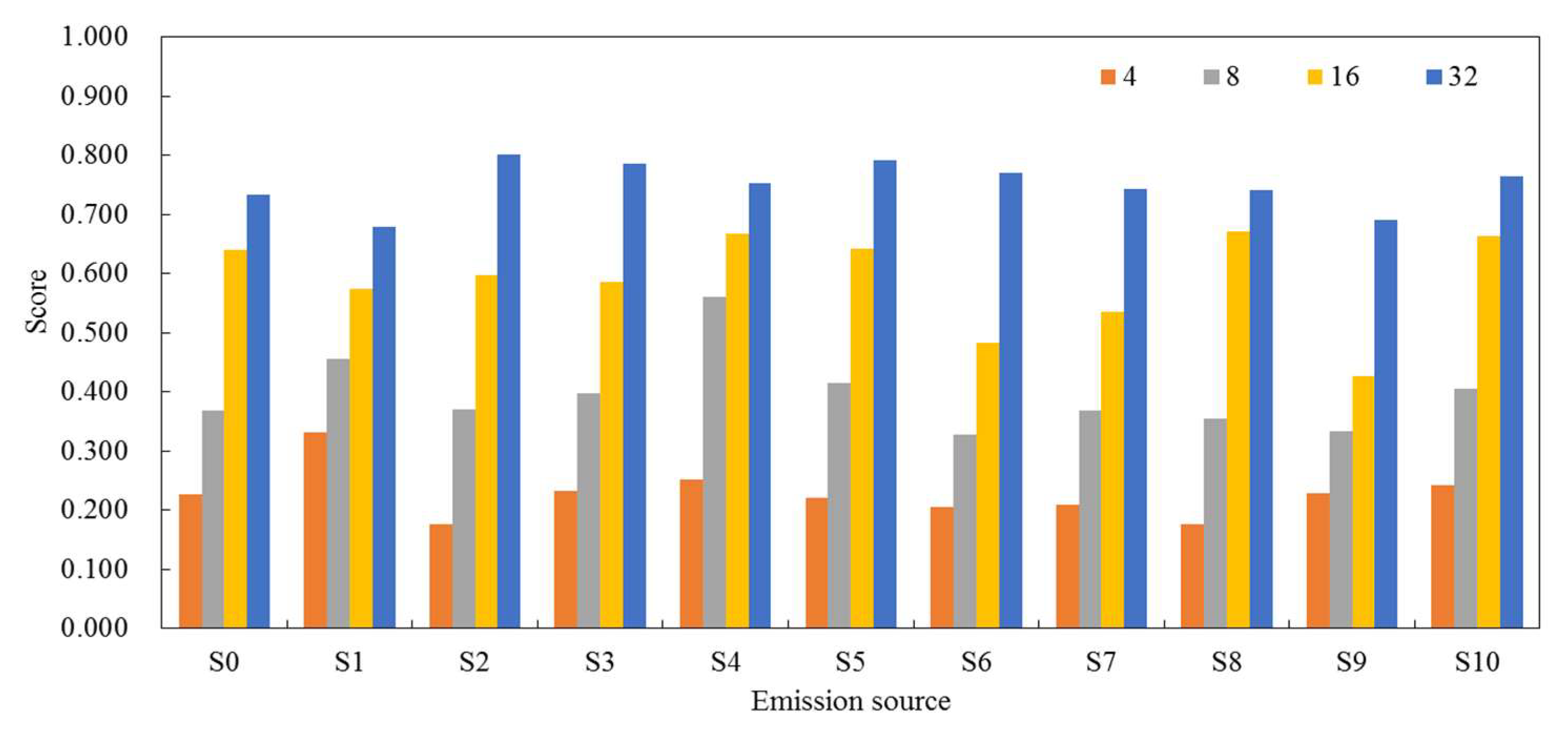
The score performances of optimal AQMNs with 4, 8, 16, 32 monitors are shown in Table 2, which were 26.06%, 45.47%, 67.74%, and 86.11% of the highest SE respectively. The SE scores for each emission source under an optimal distribution of monitors with different known number are presented in Figure 6. The results showed that SE score for each real emission source was improved with an increasing number of added monitors. In particular, the SE score for S2 increased greatly with the number of monitors. For the optimal AQMN with 4 monitors, the SE for S1 reached the highest score of 0.332, and those for the other ten sources were near 0.2. The SE scores for S4, S8, and S2 reached the highest scores for the optimal AQMNs with 8, 16, and 32 monitors, respectively.

3.2.2. Scenario II

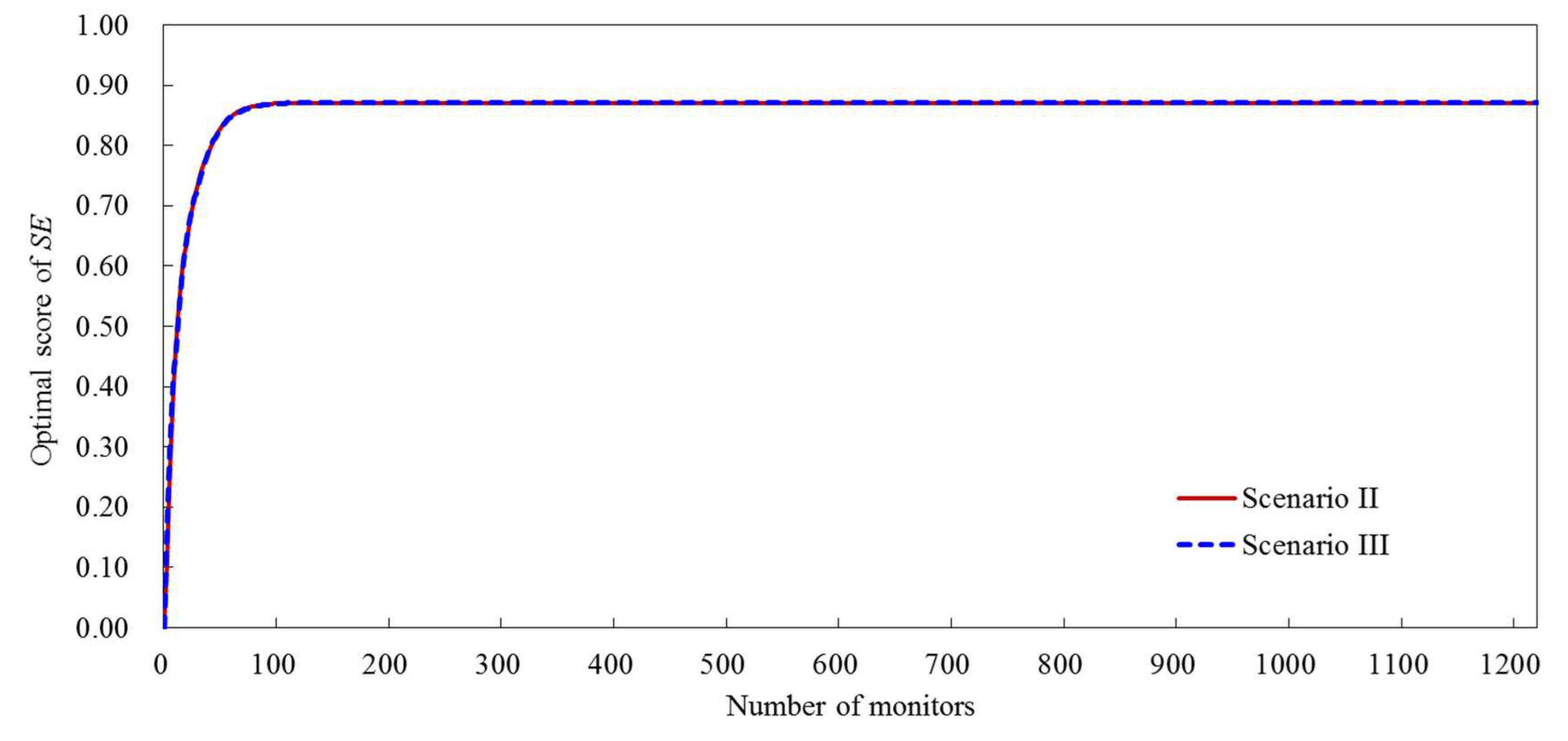
The best performances of the AQMN based on two existing monitors with an increasing number of added monitors are shown as the red line in Figure 7. The results showed that the SE was progressively enhanced with an increasing number of added monitors and reached the highest score of 0.871 when the number of monitors was about 110. Noted that the SE reached about 0.854 when the number of monitors was 64 after stepped growth. The increment was less than 0.001 after the 46th iteration, so the SE was not improved obviously. In comparison, the scheme with 64 monitors can achieve 98.05% of the optimal efficiency with nearly half the number of monitors relative to the optimal scheme (Table 2). Thus, the suggested number of monitors was considered to be 64 when M1 and M2 were fixed in this parks.
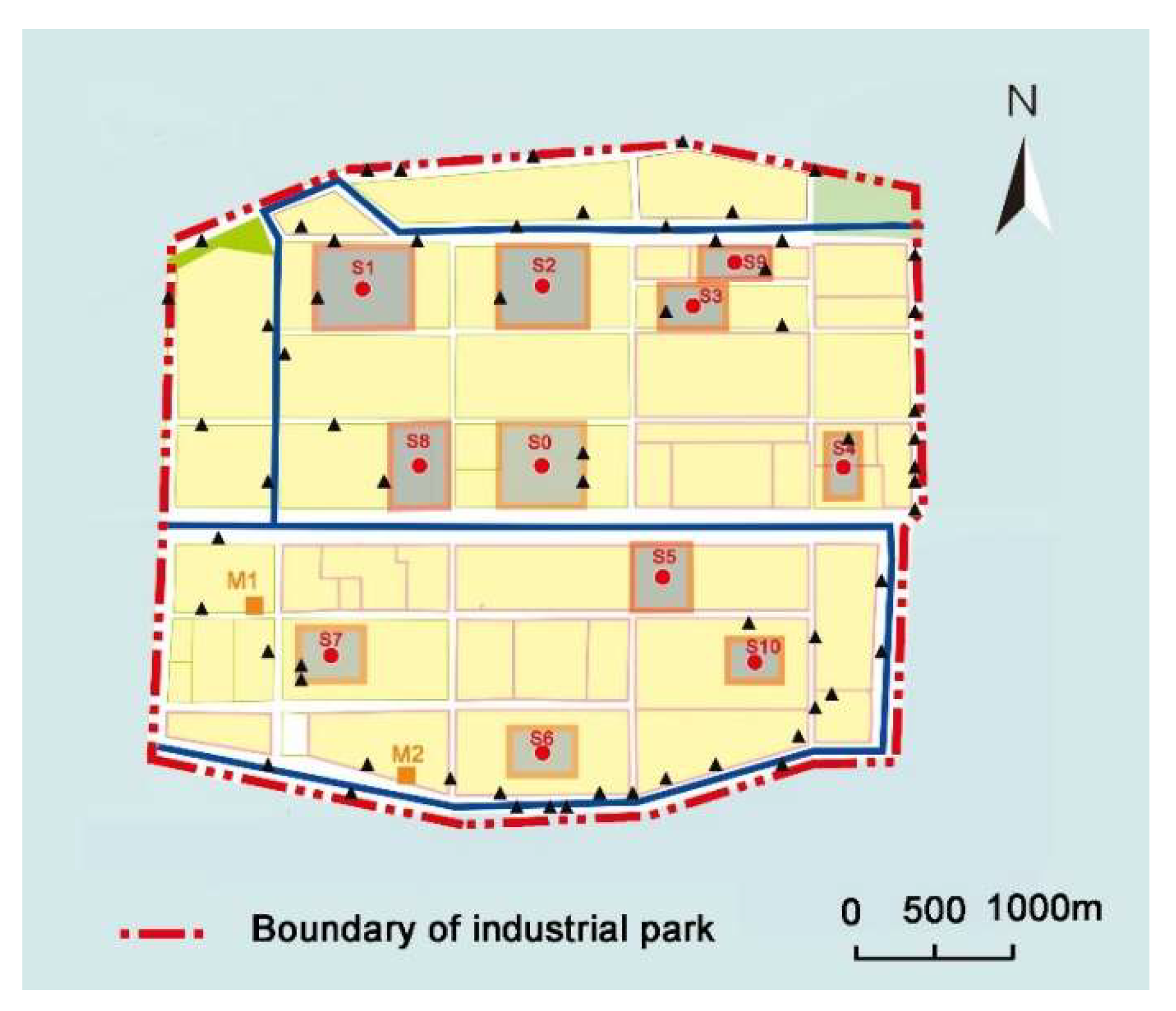
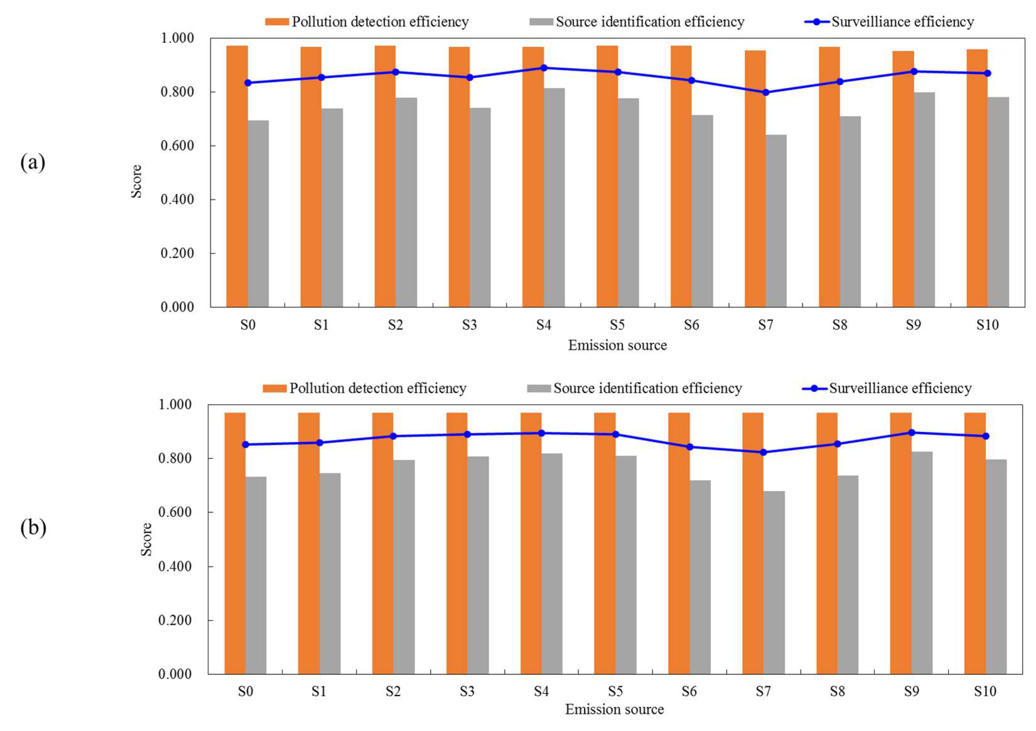
Figure 8 shows the distribution of the optimal AQMN with 64 monitors. Noted that some potential sites near sources inside this park were selected when sufficiently many monitors were provided. The corresponding score performance is presented in Figure 9a. The SE score for each real source was not lower than 0.797 for this optimal AQMN with 64 monitors. Meanwhile, the rd score for each source was not lower than 0.952, close to 1, and the rb score for each source was not lower than 0.640. It means that less than one fake source on average disturbed the back-calculation in this case, which is considered as the results given by precise source identification for this AQMN. In addition, the performance of the optimal scheme with 110 monitors (presented in Figure 9b) was basically similar to that with 64 monitors, so the additional 46 monitors were considered to be inefficient or redundant. Thus, this optimal scheme for the AQMN with 64 monitors was considered as a preferable scheme with low cost.

3.2.3. Scenario III

In Scenario III, M1 and M2 were not considered as fixed sites but as sites which were also needed to be redistributed. As shown in Figure 7, the SE scores in Scenario III were slightly higher than those in Scenario II when the number of monitors was limited, while the differences between them tended to be smaller with an increasing number of given monitors (Figure 7). We note that the increment of SE variation began to be less than 0.001 when the number of monitors is 62 after a stepped growth. Similarity, the suggested number of AQMN was 62 when two existing monitors were redistributed. The SE also reached the same highest score when the number of monitors was 110 in Scenario III. Comparisons between the performance of two existing monitors and the redistributed AQMN with two monitors in Scenario III indicate that a higher SE score can be obtained when two existing monitors are redistributed (Table 1).
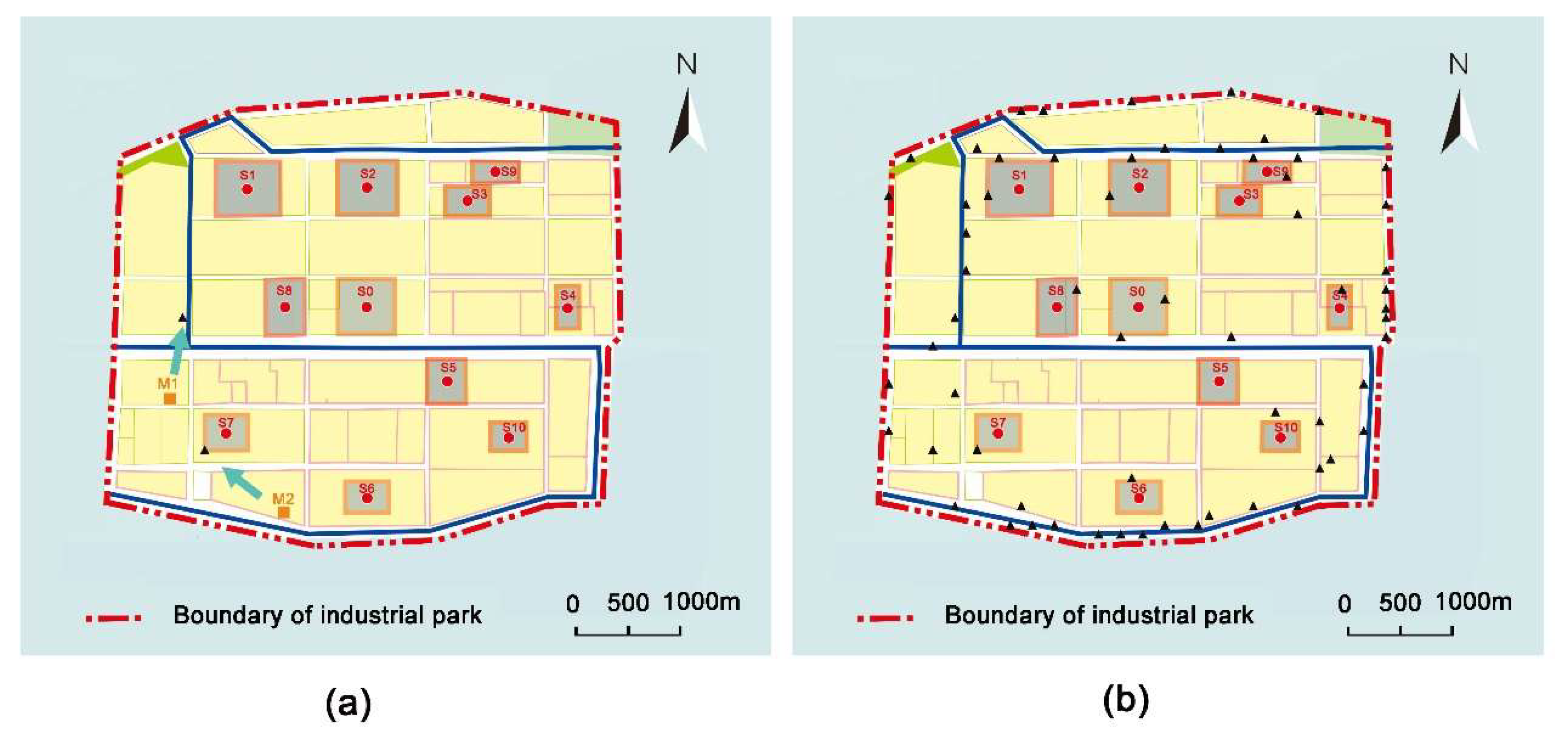
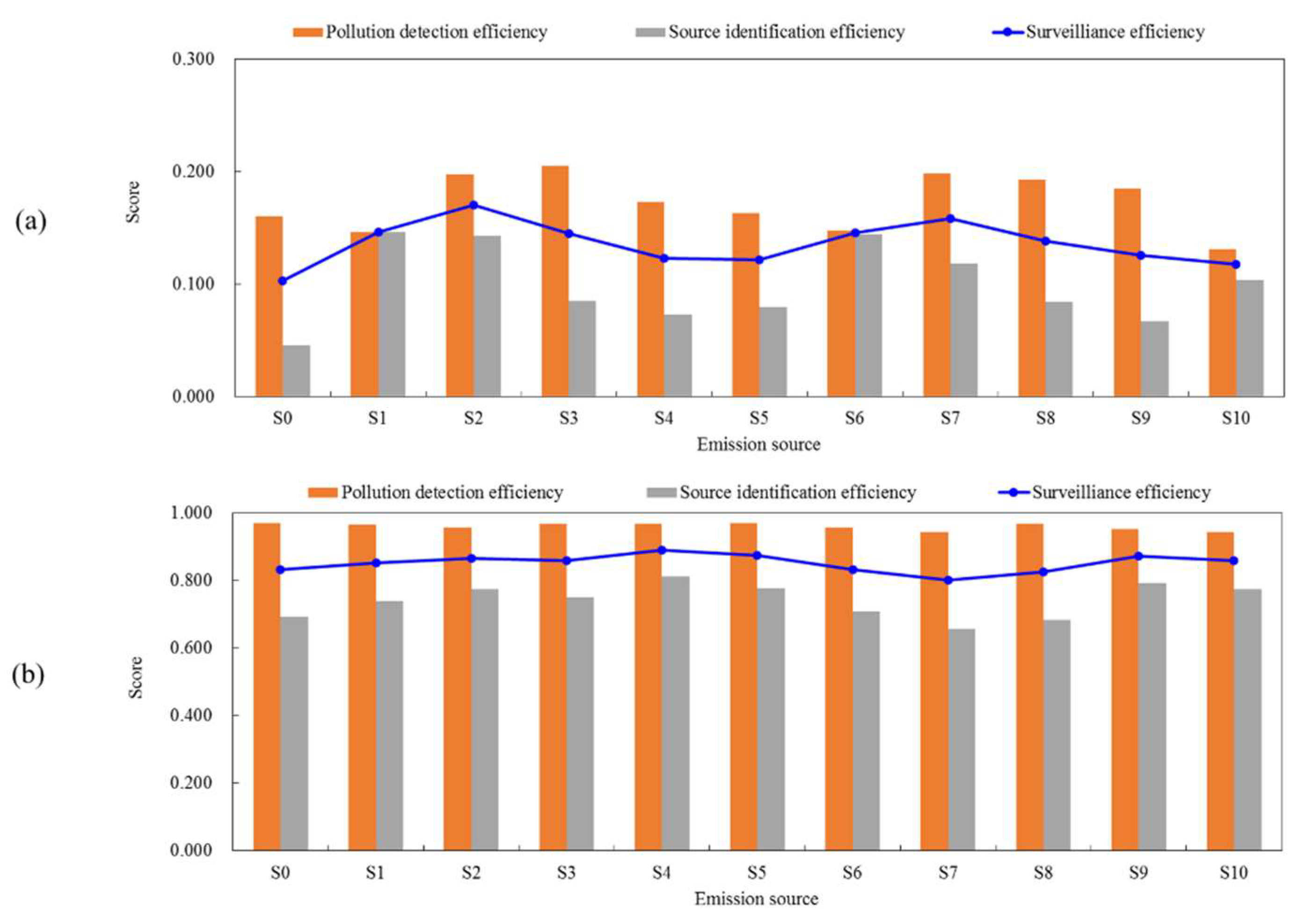
The spatial distribution of the redistributed AQMN with two monitors and the optimal AQMN with 62 monitors in Scenario III are provided in Figure 10, and the corresponding score performances are presented in Figure 11. According to the redistributed scheme, the two existing monitors were relocated to the west and southwest of this park for the highest SE performance (as shown in Figure 10a). In addition, a comparison between Figure 4c and Figure 11a shows that the performances for S2, S6, and S7 were improved obviously when the two monitors were redistributed. Figure 11b shows that the performance of the optimal AQMN with 62 monitors for Scenario III reached about 98% of the highest SE as well as that for Scenario II.

3.3. Discussion

The design objective in this article was the average of rd and rb, so the variations characteristics of the design objective were different from those in our previous study. In our previous study, monitors were preferrentially added in downwind of wind directions with higher frequencies, so rd variations were almost the same as the characteristics of wind direction probability. The performances of both rd and rb were considered here in the placement of monitors. When the number of monitors was 16, rd and rb were 0.688 and 0.491, respectively. Such back-calculation efficiency is relatively desirable. rd reached the highest score until the number of monitors was 64, owing to the consideration of rb.
Theoretically, the highest SE score is 1 if the deployed monitors are dense enough, while the highest SE score was 0.871 in our optimization (Figure 6). That is because pollution episodes under calm wind conditions (with a probability of about 2.94%) were not considered in our calculation. In addition, the rb for a single pollution episode had difficulty reaching 1 under some extremely low-wind conditions even when the number of monitors was 1221.
As shown in Table 2, rb increased more slowly than rd with the number of monitors because the influence factors of them were not exactly the same. The main influence factor of rd is the frequencies of wind directions. It depends mainly on whether there are available monitors downwind of the corresponding wind direction that may capture the pollution episode, while the number of fake sources was also considered simultaneously in the calculation of rb. Although both the efficiency of pollution detection and source identification increased with the number of monitors, rd was 1 for a single pollution episode once the episode was captured by one monitor, while the necessary number of monitors for extremely precise source identification (only a real source was covered by the back-calculated source area) is always difficult to reach.
Only constant emission rate for a whole year was considered for all eleven sources. Emission rate is a key factor for the concerned design objective, which have significant influence on the efficiency of pollution detection and source identification. Because both horizontal and vertical extensions of the envelope increase with the pre-set intensity, then more monitors may be covered by the envelope. However, emission inventories of H2S in the park is not available because abnormal emission episodes caused by such an odor pollutant are irregular and with high uncertainty. The influence of emission rate on resulting optimized network would be further analyzed in the future. In addition, according to available information about this park, it is hard to determine the weights of eleven sources. Thus only the equal weight was given in our design. More about sensitivity of spatial variation about eleven sources on optimal scheme would be further considered when more information about potential enterprises in this park is available.

4. Conclusions

A dense AQMN for H2S in a chemical industrial park was designed in this paper. SE consisting of rd and rb was considered as the design objective. The influences of long-term meteorological conditions and each emission source were considered. An evaluation of two existing monitors and optimal design schemes for three application scenarios were presented.
Two existing monitors were suggested to be relocated to the west and southwest of this park for highest SE (Figure 10a). The SE performances of optimal AQMNs with 4, 8, 16, 32 monitors were 26.06%, 45.47%, 67.74%, and 86.11% of the highest SE (0.871) respectively. The SE score of optimized AQMN increased quickly with the monitor number, and then the growth trend started to flatten when the number reached 64 for Scenario II and 62 for Scenario III. The highest SE was 0.871, which occurred when the number reached 110. Optimal scheme of an AQMN with 64 monitors was suggested when two existing monitors were fixed (Figure 8), and an optimal scheme of an AQMN with 62 monitors was preferred when two existing monitors were redistributed (Figure 10b), because they can achieve about 98% of the highest SE with only half the number of monitors of that with the highest SE.
Overall, the redistributed and optimal results demonstrated the proposed method is an effective tool in different application scenarios for designing AQMN with optimal surveillance efficiency. It is also suitable for other industrial parks. Future work is needed to design optimal AQMN considering multi-pollutants emissions and multi-sources reconstruction.

Author Contributions

Z.H. calculated the data and wrote this paper; L.C. and Q.Y. reviewed the general idea in this paper; Y.L. provided constructive discussions; W.M. made some suggestions for this the paper.

Acknowledgments

This study was supported by the project of Science and Technology Commission of Shanghai Municipality (No. 15DZ1205303).

Conflicts of Interest

The authors declare no conflict of interest.

Appendix A

This section presented the performances of Tm,e,i (Equation (5)) and Ve,m (Equation (8)) of integrated M1 and M2 for different source emissions under different meteorological conditions.
Figure A1. Tm,e,i of integrated M1 and M2 for different source emissions under different meteorological conditions.
Atmosphere 10 00318 g0a1
Figure A2. Ve,m of integrated M1 and M2 for different source emissions under different meteorological conditions.
Atmosphere 10 00318 g0a2

References

  1. Lozano, A.; José, U.; Vanderlinden, E.; Raez, J.; Contreras, J.; Navarrete, B. Optimization of the design of air quality monitoring networks and its application to NO2 and O3 in Jaen, Spain. Microchem. J. 2010, 96, 406–411. [Google Scholar] [CrossRef]
  2. Zheng, J.; Feng, X.; Liu, P.; Zhong, L.; Lai, S. Site location optimization of regional air quality monitoring network in China: Methodology and case study. J. Environ. Monit. 2011, 13, 3185–3195. [Google Scholar] [CrossRef] [PubMed]
  3. Nejadkoorki, F.; Nicholson, K.; Hadad, K. The design of long-term air quality monitoring networks in urban areas using a spatiotemporal approach. Environ. Monit. Assess. 2011, 172, 215–223. [Google Scholar] [CrossRef] [PubMed]
  4. Pope, R.; Wu, J. A multi-objective assessment of an air quality monitoring network using environmental, economic, and social indicators and GIS-based models. J. Air Waste Manag. Assoc. 2014, 64, 721–737. [Google Scholar] [CrossRef] [PubMed] [Green Version]
  5. Al-Adwani, S.; Elkamel, A.; Duever, T.A.; Yetilmezsoy, K.; Abdul-Wahab, S.A. A surrogate-based optimization methodology for the optimal design of an air quality monitoring network. Can. J. Chem. Eng. 2015, 93, 1176–1187. [Google Scholar] [CrossRef]
  6. Araki, S.; Iwahashi, K.; NShimadera, H.; Yamamoto, K.; Kondo, A. Optimization of air monitoring networks using chemical transport model and search algorithm. Atmos. Environ. 2015, 122, 22–30. [Google Scholar] [CrossRef] [Green Version]
  7. Zhao, L.; Xie, Y.; Wang, J.; Xiang, X. A performance assessment and adjustment program for air quality monitoring networks in Shanghai. Atmos. Environ. 2015, 122, 382–392. [Google Scholar] [CrossRef]
  8. Benis, K.Z.; Fatehifar, E.; Shafiei, S.; Nahr, F.K.; Purfarhadi, Y. Design of a sensitive air quality monitoring network using an integrated optimization approach. Stoch. Environ. Res. Risk Assess. 2016, 30, 779–793. [Google Scholar] [CrossRef]
  9. Orłowski, A.; Marć, M.; Namieśnik, J.; Tobiszewski, M. Assessment and Optimization of Air Monitoring Network for Smart Cities with Multicriteria Decision Analysis. In Intelligent Information and Database Systems; Nguyen, N., Tojo, S., Nguyen, L., Trawiński, B., Eds.; Springer: Cham, Switzerland, 2011; Volume 10192. [Google Scholar]
  10. Mousavi, M.S.; Ashrafi, K.; Motlagh, M.S.P.; Niksokhan, M.H.; Vosoughifar, H.R. Design of a correlated validated CFD and genetic algorithm model for optimized sensors placement for indoor air quality monitoring. Heat Mass Transf. 2018, 54, 509–521. [Google Scholar] [CrossRef]
  11. Hao, Y.; Xie, S. Optimal redistribution of an urban air quality monitoring network using atmospheric dispersion model and genetic algorithm. Atmos. Environ. 2018, 177, 222–233. [Google Scholar] [CrossRef]
  12. Chen, C.H.; Liu, W.L.; Chen, C.H. Development of a multiple objective planning theory and system for sustainable air quality monitoring networks. Sci. Total Environ. 2006, 354, 1–19. [Google Scholar] [CrossRef] [PubMed]
  13. Beaulant, A.L.; Perron, G.; Kleinpeter, J.; Weber, C.; Ranchin, T.; Wald, L. Adding virtual measuring stations to a network for urban air pollution mapping. Environ. Int. 2008, 34, 599–605. [Google Scholar] [CrossRef] [PubMed] [Green Version]
  14. Wu, L.; Bocquet, M. Optimal redistribution of the background ozone monitoring stations over France. Atmos. Environ. 2011, 45, 772–783. [Google Scholar] [CrossRef] [Green Version]
  15. Henriquez, A.; Osses, A.; Gallardo, L.; Resquin, M.D. Analysis and optimal design of air quality monitoring networks using a variational approach. Tellus Ser. B Chem. Phys. Meteorol. 2015, 67. [Google Scholar] [CrossRef] [Green Version]
  16. Gupta, S.; Pebesma, E.; Mateu, J.; Degbelo, A. Air quality monitoring network design optimisation for robust land use regression models. Sustainability 2018, 10, 1442. [Google Scholar] [CrossRef]
  17. Sharan, M.; Singh, S.K.; Issartel, J.P. Least square data assimilation for identification of the point source emissions. Pure Appl. Geophys. 2012, 169, 483–497. [Google Scholar] [CrossRef]
  18. Turbelin, G.; Singh, S.K.; Issartel, J.P. Reconstructing source terms from atmospheric concentration measurements: Optimality analysis of an inversion technique. J. Adv. Model. Earth Syst. 2014, 6, 1244–1255. [Google Scholar] [CrossRef]
  19. Hosseini, B.; Stockie, J.M. Bayesian estimation of airborne fugitive emissions using a gaussian plume model. Atmos. Environ. 2016, 141, 122–138. [Google Scholar] [CrossRef]
  20. Efthimiou, G.C.; Kovalets, I.V.; Venetsanos, A.; Andronopoulos, S.; Argyropoulos, C.D.; Kakosimos, K. An optimized inverse modelling method for determining the location and strength of a point source releasing airborne material in urban environment. Atmos. Environ. 2017, 170, 118–129. [Google Scholar] [CrossRef]
  21. Huang, Z.; Qi, Y.; Ma, W.; Chen, L. Surveillance efficiency evaluation of air quality monitoring networks for air pollution episodes in industrial parks: Pollution detection and source identification. Atmos. Environ. 2019. Under Review. [Google Scholar]
  22. Flesch, T.K.; Wilson, J.D.; Harper, L.A. Deducing ground-to-air emissions from observed trace gas concentrations: A field trial with wind disturbance. J. Appl. Meteorol. 2005, 43, 487–502. [Google Scholar] [CrossRef]
  23. Chow, F.K.; Kosović, B.; Chan, S. Source inversion for contaminant plume dispersion in urban environments using building-resolving simulations. J. Appl. Meteorol. Climatol. 2008, 47, 1553–1572. [Google Scholar] [CrossRef]
  24. Long, K.J.; Haupt, S.E.; Young, G.S. Assessing sensitivity of source term estimation. Atmos. Environ. 2010, 44, 1558–1567. [Google Scholar] [CrossRef]
  25. Rodriguez, L.M.; Haupt, S.E.; Young, G.S. Impact of sensor characteristics on source characterization for dispersion modeling. Measurement 2011, 44, 802–814. [Google Scholar] [CrossRef]
  26. Kovalets, I.V.; Andronopoulos, S.; Venetsanos, A.G.; Bartzis, J.G. Identification of strength and location of stationary point source of atmospheric pollutant in urban conditions using computational fluid dynamics model. Math. Comput. Simul. 2011, 82, 244–257. [Google Scholar] [CrossRef]
  27. Ma, D.L.; Deng, J.Q.; Zhang, Z.X. Comparison and improvements of optimization methods for gas emission source identification. Atmos. Environ. 2013, 81, 188–198. [Google Scholar] [CrossRef]
  28. Ma, D.L.; Zhang, Z.X. Contaminant dispersion prediction and source estimation with integrated gaussian-machine learning network model for point source emission in atmosphere. J. Hazard. Mater. 2016, 311, 237–245. [Google Scholar] [CrossRef] [PubMed]
  29. Duyzer, J.; Dick, V.D.H.; Zandveld, P.; Van Ratingen, S. Representativeness of air quality monitoring networks. Atmos. Environ. 2015, 104, 88–101. [Google Scholar] [CrossRef]
  30. Kumar, P.; Feiz, A.A.; Ngae, P.; Singh, S.K.; Issartel, J.P. CFD simulation of short-range plume dispersion from a point release in an urban like environment. Atmos. Environ. 2015, 122, 645–656. [Google Scholar] [CrossRef] [Green Version]
  31. Kumar, P.; Singh, S.K.; Feiz, A.A.; Ngae, P. An urban scale inverse modelling for retrieving unknown elevated emissions with building-resolving simulations. Atmos. Environ. 2016, 140, 135–146. [Google Scholar] [CrossRef] [Green Version]
  32. Huang, Z.; Yuan, W.; Qi, Y.; Ma, W.; Yan, Z.; Chen, L. Source area identification with observation from limited monitor sites for air pollution episodes in industrial parks. Atmos. Environ. 2015, 122, 1–9. [Google Scholar] [CrossRef]
  33. MODEL T101 UV FLUORESCENCE23 H2S ANALYZER. 2016. Available online: http://www.teledyne-api.com/prod/Downloads/07266C%20-%20T101%20Manual.pdf#search=User%20MANUAL%20MODEL%20T101%20UV%20FLUORESCENCE (accessed on 11 May 2019).
  34. Arbeloa, F.J.S.; Caseiras, C.P.; Andrés, P.M.L. Air quality monitoring: Optimization of a network around a hypothetical potash plant in open countryside. Atmos. Environ. Part A Gen. Top. 1993, 27, 729–738. [Google Scholar] [CrossRef]
  35. Jiang, W. Air Pollution Meteorology; Nanjing University Press: Nanjing, China, 2003; pp. 124–125. [Google Scholar]
  36. MEEPRC (Ministry of Ecology and Environment of the People’s Republic of China). Technical Guidelines for Environmental Risk Assessment on Projects (HJ/T 169-2004). 2004. Available online: http://kjs.mee.gov.cn/hjbhbz/bzwb/other/pjjsdz/200412/W020110127329297430823.pdf (accessed on 11 May 2019).
  37. MEEPRC (Ministry of Ecology and Environment of the People’s Republic of China). Technical Methods for Making Local Emission Standards of Air Pollutants (GB/T3840-91). 1991. Available online: http://www.mee.gov.cn/image20010518/5332.pdf (accessed on 11 May 2019).
  38. Petty, G.W. A First Course in Atmospheric Thermodynamics; Sundog Pub.: Madison, WI, USA, 2008; p. 33. [Google Scholar]
  39. Venkatram, A.; Klewicki, J. Validation of Concentrations Estimated from Air Dispersion Modeling for Source-Receptor Distances of Less than 100 Meters; California Air Resources Board, Research Division: Sacramento, CA, USA, 2003. [Google Scholar]
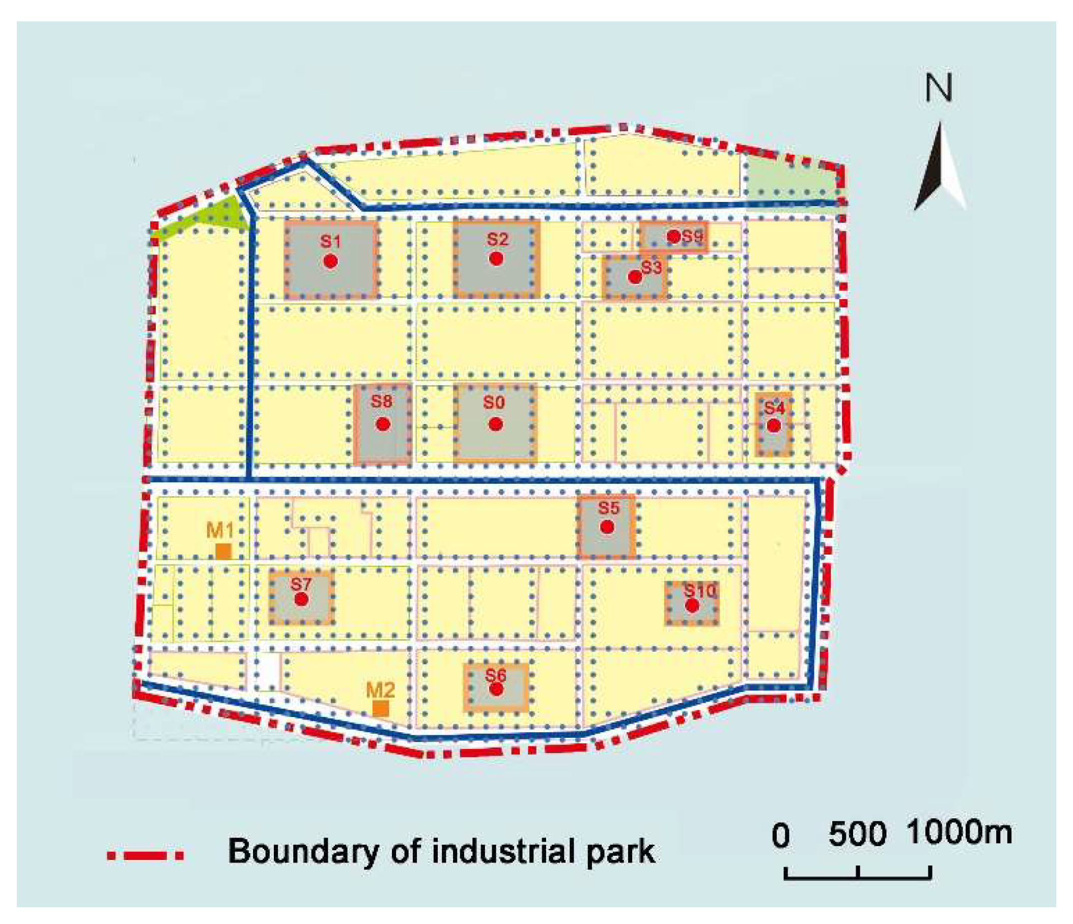
Figure 1. Distributions of sources and monitors in the industrial park. Eleven sources (S0–S10) are denoted by red dots. The locations of existing monitors (M1 and M2) are denoted by orange squares. The arrangements of more candidate monitors are indicated by blue dots.
Atmosphere 10 00318 g001
Figure 2. Meteorological conditions for the study area. (a) Joint frequency distributions of wind direction and speed and (b) frequency distribution of atmospheric stability.
Atmosphere 10 00318 g002
Figure 3. Flowchart of proposed method for optimal design of a dense AQMN.
Atmosphere 10 00318 g003
Figure 4. The individual and integrated performances of M1 and M2 for different real emission sources. (a): M1; (b): M2; (c):M1 and M2.
Atmosphere 10 00318 g004
Figure 5. The spatial distributions of the optimal air quality monitoring networks (AQMNs) with different known numbers of monitors. Orange squares indicate two existing monitors, and black triangles indicate added monitors in the optimal scheme. The numbers of monitors are (a) 4, (b) 8, (c) 16, and (d) 32.
Atmosphere 10 00318 g005
Figure 6. Surveillance Efficiency (SE) scores of each emission source under optimal AQMNs with different known numbers.
Atmosphere 10 00318 g006
Figure 7. Optimal SE scores for AQMNs with different numbers of monitors. The red line represents the result of Scenario II; the blue line represents the result of Scenario III.
Atmosphere 10 00318 g007
Figure 8. The spatial distribution of the optimal AQMN with 64 monitors. Orange squares indicate two existing monitors, and black triangles indicate added monitors in the optimal scheme.
Atmosphere 10 00318 g008
Figure 9. The performance of the optimal distribution of the AQMN for Scenario II. The numbers of monitors are (a) 64 and (b) 110.
Atmosphere 10 00318 g009
Figure 10. The spatial distribution of the optimal AQMN in Scenario III. Black triangles indicate added monitors in the optimal scheme. The numbers of monitors are (a) 2 and (b) 62.
Atmosphere 10 00318 g010
Figure 11. SE scores of the optimal AQMNs for different real sources in Scenario III. The numbers of monitors are (a) 2 and (b) 62.
Atmosphere 10 00318 g011
Table 1. Score performance of two existing monitors and optimal AQMN (air quality monitoring network) with two monitors.
MonitorsrdrbSESE/SEmax
M10.0770.0360.0576.54%
M20.0710.0360.0536.09%
M1 and M20.1460.0720.10912.51%
Optimal AQMN with two monitors0.1730.0990.13615.61%
Table 2. Score performances of AQMNs with different number of monitors.
Number of MonitorsrdrbSESE/SEmax
40.2960.1580.22726.06%
80.4920.2990.39645.47%
160.6880.4910.59067.74%
320.8630.6380.75086.11%
640.9650.7440.85498.05%
1100.9710.7710.871100%
12210.9710.7710.871100%